the Creative Commons Attribution 4.0 License.
the Creative Commons Attribution 4.0 License.
 | 01 Aug 2018
North Atlantic subpolar gyre along predetermined ship tracks since 1993: a monthly data set of surface temperature, salinity, and density
Gilles Reverdin
Hedinn Valdimarsson
Gael Alory
Denis Diverres
Francis Bringas
Gustavo Goni
Lars Heilmann
Leon Chafik
Tanguy Szekely
Andrew R. Friedman
We present a binned product of sea surface temperature, sea surface salinity, and sea surface density data in the North Atlantic subpolar gyre from 1993 to 2017 that resolves seasonal variability along specific ship routes (https://doi.org/10.6096/SSS-BIN-NASG). The characteristics of this product are described and validated through comparisons to other monthly products. Data presented in this work were collected in regions crossed by two predetermined ship transects, between Denmark and western Greenland (AX01) and between Iceland, Newfoundland, and the northeastern USA (AX02). The data were binned along a selected usable transect. The analysis and the strong correlation between successive seasons indicate that in large parts of the subpolar gyre, the binning approach is robust and resolves the seasonal timescales, in particular after 1997 and in regions away from the continental shelf. Prior to 2002, there was no winter sampling over the West Greenland Shelf. Variability in sea surface salinity increases towards Newfoundland south of 54∘ N, as well as in the western Iceland Basin along 59∘ N. Variability in sea surface temperature presents less spatial structure with an increase westward and towards Newfoundland. The contribution of temperature variability to density dominates in the eastern part of the gyre, whereas the contribution of salinity variability dominates in the southwestern part along AX02.


Francis Bringas' and Gustavo Goni's copyright for this publication is transferred to the National Oceanic and Atmospheric Administration (NOAA)..
The North Atlantic subpolar gyre (NASPG) has been extensively studied and observed during the last 25 years. This time span presents the succession of a cold period in the early 1990s associated with strong North Atlantic Oscillation (NAO) forcing, a warmer period from 2000 to 2009, followed by a cooling (Robson et al., 2016), and strong NAO forcing in 2014 and 2015 (Josey et al., 2017). These conditions were associated with strong variability in intermediate water formed in the Labrador Sea, southwestern Irminger Sea, and south of Greenland, with strong formation years following strong atmospheric and NAO forcing years (Yashayaev and Loder, 2016; Fröb et al., 2016; De Jong and de Steur, 2016; Piron et al., 2017). There has also been extensive variability in mode waters and their thickness in the northern and northeastern subpolar gyre, such as the Reykjanes mode water (Thierry et al., 2008) or the Rockall Trough mode water (Holliday et al., 2015). The changes in these subsurface water properties and distributions drive ocean circulation and in particular play a likely role in the Atlantic Meridional Overturning Circulation (AMOC) variability (Robson et al., 2016; Rahmstorf et al., 2015). The surface layer provides the link between the ocean interior and the atmosphere.
Surface variability in oceanic properties responds to atmospheric forcing and ocean circulation changes. In particular, the NAO and the East Atlantic Pattern are known to strongly influence heat and freshwater fluxes in this region (Cayan, 1992; Hurrell et al., 2013; Bojariu and Reverdin, 2002) and thus sea surface temperature (SST) and sea surface salinity (SSS) (Josey and Marsh, 2005). Changes in freshwater fluxes from continental run-off and ice melt are also expected to change surface properties in the NASG (Böning et al., 2016). Net run-off from Greenland has considerably increased during the last decades (van der Broeke et al., 2016). The role of changes in ocean circulation has also been identified. For instance, the proportion of inflowing subtropical water was found to have increased in the 1995–2005 period compared to the previous 2 decades (Häkkinen et al., 2011, 2013), followed by a net reduction of this input (Robson et al., 2016), which could have contributed to the more recent decadal cooling/freshening (see also Piecuch et al., 2017). Decadal changes in the strength of the gyre circulation have been associated with zonal displacements of the subpolar front (Hatun et al., 2005; Sarafonov, 2009). This has been disputed (Foukal and Lozier, 2017), and has not been clearly identified in subsets of in situ current measurements along 59∘ N in two multi-year periods (Rossby et al., 2017), although recent analysis of altimetric sea-level data supports an eastward displacement of the subpolar front during the recent period of strong atmospheric forcing (Zunino et al., 2017; their Fig. 8). Furthermore, a strong cold blob and anomalous cooling (and freshening) area have appeared in the center of the NASPG since the late 2000s, and have also been linked indirectly to changes in the AMOC (Rahmstorf et al., 2015; Josey et al., 2017).
The strong changes in thermocline and water masses associated with displacements of the subpolar front and in the southern part of the NASPG have been used by Stendardo et al. (2016) to reconstruct surface temperature and salinity based on satellite altimetry data. However, this method does not work well in the interior of the NASPG, nor on the slopes and shelves. To complement these analyses and the very valuable coverage of the NASPG at low resolution by Argo floats, we construct monthly time series of temperature (T), salinity (S), and density along tracks in the interior of the gyre, and over the nearby shelves. The expectation is that data coverage and accuracy are good enough to resolve interannual variability at seasonal timescale since the early or mid 1990s at the ocean surface, and thus provide valuable information for studies on the interannual to decadal variability of the NASPG. This extends earlier work on data presented in Reverdin et al. (2002).
The data and methods used are first described in Sect. 2, and then the time series are presented in Sect. 3. Some statistical properties are described to illustrate the potential of the binned data to characterize interannual variability: the pattern of standard deviations, and empirical orthogonal function (EOF) analysis. Descriptions of the data validation performed and comparisons with other products are presented in the Appendices.
2.1 Data
A large part of the data presented here are from SBE21 and SBE45 thermosalinographs (TSGs) installed on cargo ships running along the AX01 transect between Denmark and western Greenland and along the AX02 transect between Iceland, Newfoundland, and the northeastern USA (Fig. 1). Along AX01, TSG data were collected on M/V Nuka Arctica between July 1997 and December 2017 (with intake temperature in 2005–2017). Along AX02, TSG data are available between April 1994 and December 2007 (with intake temperature during April 1994–1996) and between March 2011 and March 2016. Along AX02, TSG data collected in February 2003 to December 2004 were not included, as they were judged to be of irregular quality, and could not be fully validated.
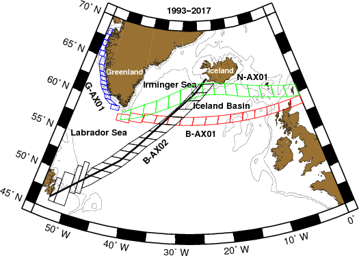
Figure 1Map of the bins along B-AX01 (red), B-AX02 (black), G-AX01 (blue), and N-AX01 (green). A typical example of a ship track is shown along B-AX02.
The first installation on Nuka Arctica was done on a pumped water circuit in the bow thruster room of the ship, with little warming but frequent interruptions during and after bad weather. In 2006, it was moved to the engine room at approximately mid-ship, roughly 5 m below the water line. During some winters (January–March 1997–2002), Nuka Arctica was not servicing this shipping lane. The most common route crosses the North Atlantic subpolar gyre along 59–59.5∘ N (B-AX01), but the ship has often taken a different route, in particular further north (N-AX01) (see, e.g., Chafik et al., 2014, their Fig. 1). Along western Greenland, at least north of 62∘ N, the route is fairly repeated between transects and often runs in mid-shelf between ports-of-call, very often up to southern Disko Bay (G-AX01), with a few crossings in summer further north to Thule in northwestern Greenland.
Along AX02, a succession of ships has been used, with different installations usually in the engine room at mid-ship, between 4 and 7 m below the water line. The route taken by these vessels is often roughly straight between southeastern Newfoundland and the western tip of the Reykjanes Peninsula (Fig. 1, which we will refer to as the standard route B-AX02), but with some deviations depending on sea ice or weather conditions. Due to seasonal sea ice, in particular, there were no standard TSG data on the route northeast of Newfoundland on shelf and slope in February–April 1994–1995 and 2014–2016.
The validation and correction of the TSG salinity data are mostly based on comparison with water samples collected from a water intake at the TSG (AX01 and AX02) and using nearby upper-level Argo float data (primarily for AX02) (Alory et al., 2015). On AX02, adjusting T from the TSG to near-surface ocean temperature was done when no intake measurements were available, largely based on comparison with T from expandable bathythermograph (XBT) observations at 5–7 m. XBT observations along these two transects were started in 2000 (AX01) and 1993 (AX02) and have produced approximately 4000 temperature profiles available for these comparisons. In addition, T measurements from the TSG on Nuka Arctica (AX01) were also used to adjust T along AX02 where there were crossovers of the AX01 and AX02 ship route. Validation of T and S data from the thermosalinographs is discussed further in Appendix A. For AX02, additional T and S data originate from seasonal surface sampling, in particular in July 1993, January and April 1994, in 1995, in 2003–2004, and in 2007–2017. TSG data from several research cruises were also included. Upper-level data (near 5–7 m) of profiles from Argo, earlier PALACE floats (since 1996) (Lavender et al., 2000; Davis et al., 2001), and conductivity, temperature, depth (CTD) probes were also considered, as well as data from drifters equipped to measure precise temperature and salinity.
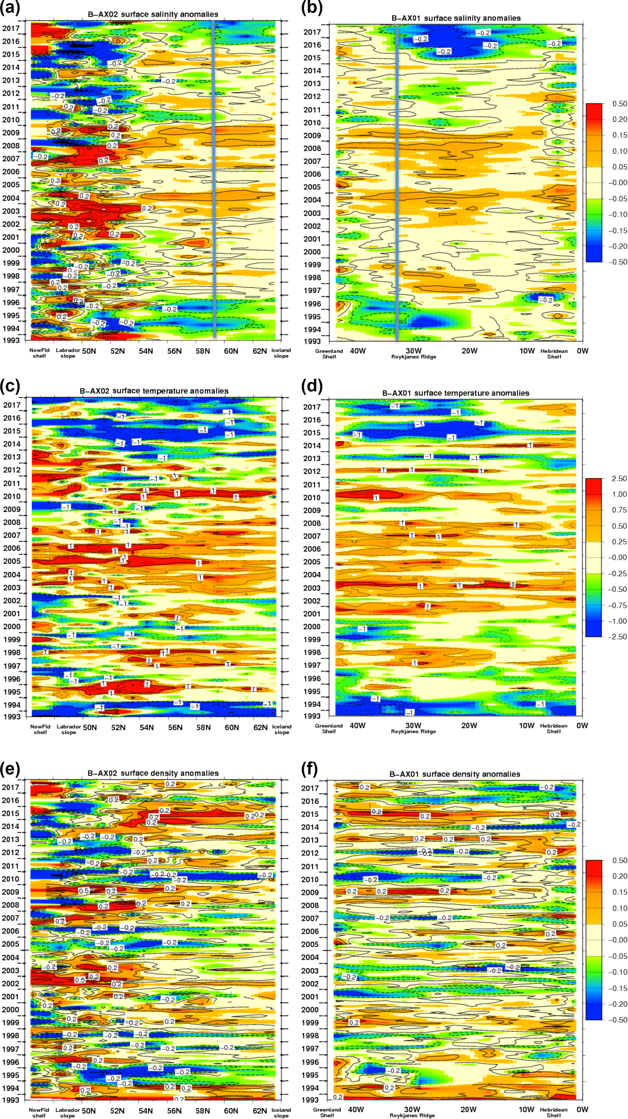
Figure 2B-AX02 (a, c, e) and B-AX01 (b, d, f) Hoevmøller diagrams of deviations from an average seasonal cycle. Salinity (a, b), temperature (c, d, ∘C), and density (e, f, kg m−3). Figure 1 indicates where the lines are located, and the vertical grey lines in the panels indicate where the two sections intersect.
2.2 Methods
We construct monthly binned temperature, practical salinity, and water density time series starting in mid 1993 along two standard sections intersecting near 59.5∘ N, 32∘ W: B-AX01 between the North Sea and South Greenland and B-AX02 between Iceland and southern Newfoundland (Fig. 1). The B-AX01 section extends from the southeast of Cape Farewell (excluding the shelf or its vicinity) to the northwestern North Sea northeast of Scotland over the shelf. A separate binning G-AX01 is done on the Greenland shelf between southern Disko Bay (near 68.2∘ N, 54∘ W) and northwest of Cape Farewell, but only since July 1996 (with no data north of 64.5∘ N in 1996–1997). We also binned data on an alternate route often used by Nuka Arctica across the Irminger Sea and Iceland Basin (N-AX01), to the north of B-AX01. For B-AX02, we include two bins over the Newfoundland shelf and two bins further to the northeast over the continental slope, followed by more regular bins along the standard section.
First, a gridded seasonal cycle is subtracted from the data to create anomalies that are then grouped in the bins on a monthly timescale. The average seasonal cycle is based on 120 years of data in the NASPG provided on a latitude × longitude grid (as in Friedman et al., 2017, and extended to salinity and temperature). After creating the temperature and salinity time series, the average seasonal cycle is adjusted so that there is no residual seasonal cycle of the anomalies over the time series length. The total values are constructed by adding the average seasonal cycle to the anomalies. Time series of surface density are estimated from the temperature and salinity time series. Time series along B-AX01 contain some long-lasting data gaps until late 1997 that were partially filled with data along 58 or 60∘ N, which therefore are attributed to larger errors. Along G-AX01, there are no winter data (January–March) in 1997–2002. Time series along B-AX02 start in July 1993, with few gaps longer than 3 months, the longest being associated with winters with ice presence over the Newfoundland shelf or slope. The time series are then smoothed by a 1–2–1 running mean over successive months. Comparison of this gridded product against other gridded products is provided in Appendix B.
3.1 Variability along AX01 and AX02
Hovmøller diagrams of seasonal salinity anomalies are presented in Fig. 2. A rather similar variability is portrayed where the two sections B-AX01 and B-AX02 intersect (with rms differences which are less than the error estimates), although clearly B-AX01 indicates a strong longitude dependence of the signals portrayed just to the east of the intersection with B-AX02.
The B-AX02 salinity plot (Fig. 2a) suggests large spatial variations characterized by interannual to decadal variability. In the shelf and slope regions, in particular near Newfoundland, there seems to be more short-term variability. However, in these regions, error estimates are also larger, to some extent as a result of insufficient sampling, as well as due to unresolved high-frequency variability. This results in weak correlation of S anomalies between successive seasons (3 months apart), although there is a tendency for negative low-frequency anomalies until 2000 and since 2010. Correlation in other regions of B-AX02 between successive seasons is larger (correlation coefficient at least 0.6), indicating a dominance of interannual and lower-frequency variability over intra-annual variability. There is less spatial variability along B-AX01 (Fig. 2a). There is a tendency for differences across the Reykjanes Ridge, such as in 1994 or 2015–2017, with large negative anomalies in the western Iceland Basin. Variability on European shelves also tends to be different. On B-AX01, correlation is also large between successive seasons, with an exception in the last 200 km from the shelf break off southern Greenland. There, however, the TSG transects do not resolve well enough the spatial and temporal variability.
Temperature anomalies (Fig. 2c, d) tend not to be correlated with the salinity ones, although there is some suggestion that the decadal variability is correlated (except on the shelves). This is seen here as the negative SST anomalies near the beginning and end of the time series with warmer temperatures in the 2000–2009 period, roughly corresponding to SSS variability of the same sign. Variability is slightly larger along B-AX02, as expected from the known westward increase in SST variability portrayed for example in the Hadley Centre SST data set (Kennedy et al., 2011a, b). Altogether there is not a large spatial variability in the temperature signals along these transects, at least on seasonal or longer timescales, except for some differences in the southern part of B-AX02 compared to other regions.
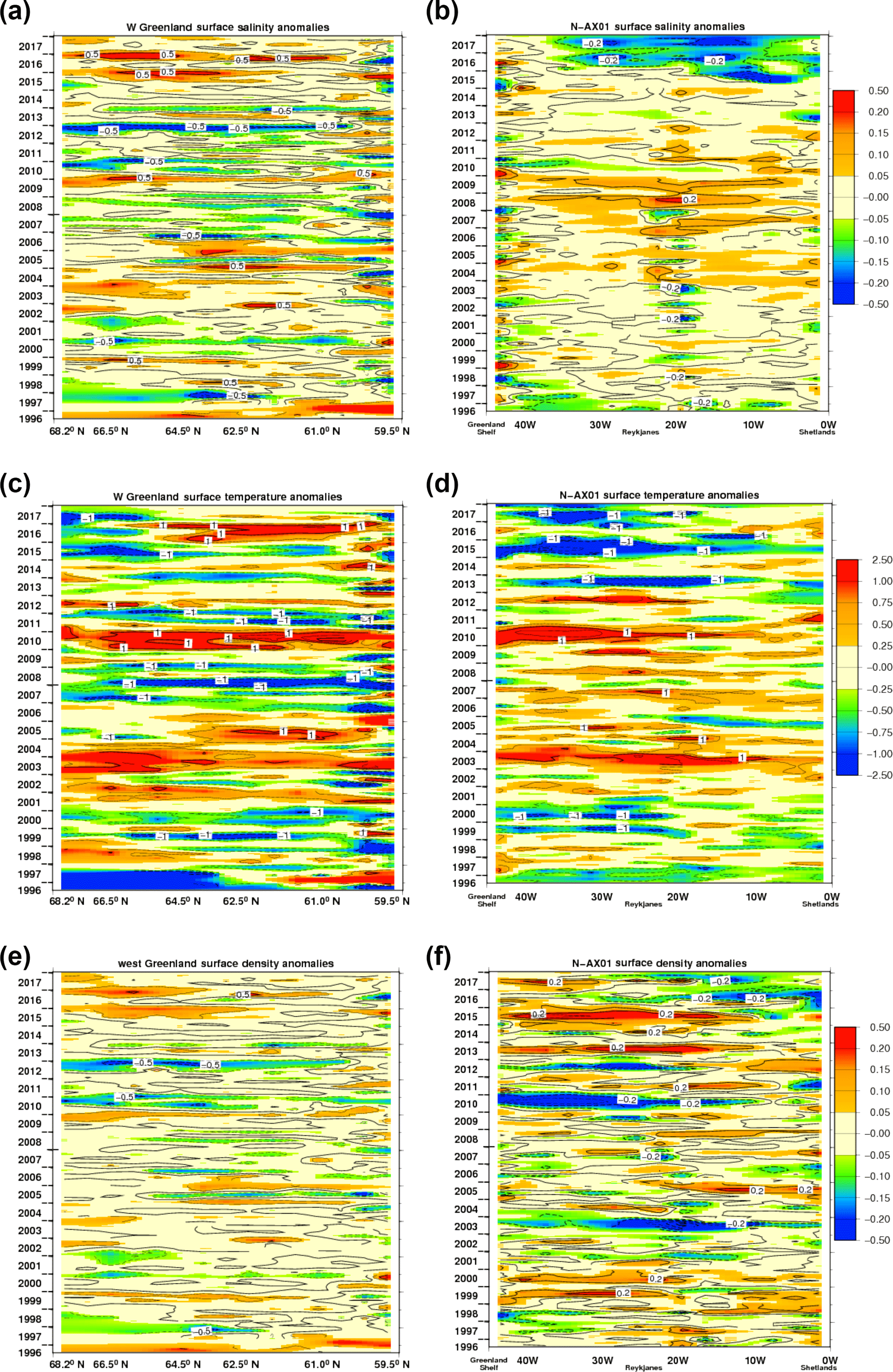
Figure 3G-AX01 (a, c, e) and N-AXO1 (b, d, f) anomalies Hoevmøller diagrams of deviations from an average seasonal cycle. Salinity (a, b), temperature (c, d, ∘C), and density (e, f, kg m−3) (see Fig. 1 for locations of sections). For salinity and density, different contours/color codes are used for G-AX01 and N-AX01.
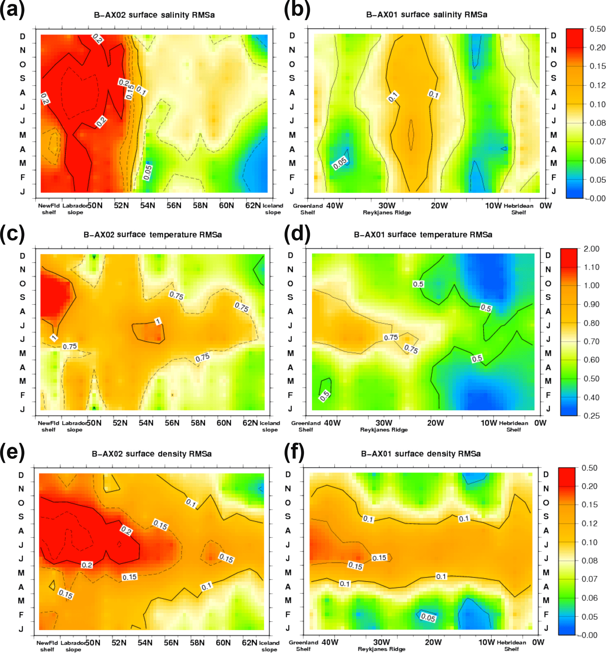
Figure 4Seasonal cycle of interannual variability standard deviation RMSa: (a, c, e) along B-AX02; (b, d, f) along B-AX01. S (a, b), T (c, d, ∘C), and density (e, f, kg m−3).
Density anomalies (Fig. 2e, f) are a result of both temperature and salinity anomalies. Except in the southern part of B-AX02 (south of 54∘ N), temperature variability tends to have a larger contribution than salinity variability to density (in particular east of the Reykjanes Ridge in the Iceland Basin or north of 60∘ N). Thus, as for T, density anomalies along B-AX01 tend to present small longitudinal variations, in particular with the highest positive density anomalies in the first few years and from mid 2014 to early 2016. Since early 2016, negative density anomalies have been confined east of the Reykjanes Ridge. Along B-AX02, there is a larger contrast, with a transition near 52–54∘ N, with the density anomalies looking more like S south of it and more like T north of it. The correlation between density anomalies in successive seasons is also smaller for surface density than for T and S.
To a large extent, section N-AX01 (Fig. 3) presents variability that is coherent with what is seen on B-AX01 along 59∘ N (Fig. 2). However, whereas in the Iceland Basin near 10–18∘ W along N-AX01, one also finds the freshening happening by mid 2015, further west (and closer to Iceland) as well as in the northeastern Irminger Sea east of 35∘ W, the freshening happens later in 2016 and 2017 (with some suggestion of a weaker winter signal). This freshening did not show up along 59∘ N (B-AX01) in the eastern Irminger Sea away from the Reykjanes Ridge until late 2017 (Fig. 2). Along N-AX01, at 20∘ W, very close to southern Iceland, there are also isolated patches of larger anomalies, possibly related to local freshwater inputs from Iceland. To the east of the section, the last bin near the Shetland Islands portrays a variability often very close to what is found further west in the deeper ocean, whereas the two easternmost bins of section B-AX01 on the shelf (northwest and northeast of Scotland) seem to present a different variability.
Finally, variability on the southwestern West Greenland Shelf (G-AX01, Fig. 3) is rather different for S than further east in the Irminger Sea along B-AX01 or N-AX01. Except for the southernmost box to the west of Cape Farewell, variability in S is rather coherent meridionally. For example, negative anomalies are observed in 2000, from mid 2006 to early 2009, and even more in 2010–2013, with a peak in the second half of 2012, and positive anomalies in 2015–2017. The extreme negative S values in late 2012 are consistent with the outstanding Greenland ice sheet melt that occurred that year (van der Broeke et al., 2016; Fettweis et al., 2017). On the other hand, other years with very large southern Greenland ice sheet melt (1995, 2002, 2005–2007, 2010, 2011) do not show as well in surface salinity. Temperature variability tends to be also of the same sign along the section, but with some notable exceptions. For instance, negative T anomalies are found in 2015–2017 north of 65∘ N, and not further south.
3.2 Seasonal cycle of the standard deviation of interannual variability
For each month of the calendar year, we evaluate the root-mean square standard deviation of interannual variability of the anomaly time series (referred to as RMSa). We thus estimate a seasonal cycle of RMSa (Fig. 4). For S (Fig. 4a, b), large RMSa values are found in the southern part of B-AX02 with a large decrease between 52 and 54∘ N from spring to autumn (between 52 and 53∘ N in winter). Near 55∘ N, there is minimum RMSa during winter–spring, and then it increases again near 57–59∘ N, followed by a strong decrease towards Iceland. RMSa salinity presents a seasonal cycle with a spring minimum over the Newfoundland shelf, which is less noticeable along the continental slope. Further offshore and until 54∘ N, there is a minimum variability in spring (and maximum during late summer/autumn). North of 54∘ N, there is a winter to late winter minimum, although poorly defined near 56–59∘ N. This winter to early spring minimum is also very prominent along N-AX01, except in the western Irminger Sea, close to the Greenland shelves (not shown). Along B-AX01 at 59∘ N (B-AX01) for S, maximum RMSa is found in the western Iceland Basin (20–30∘ W), and then it decreases further east (as well as in the Irminger Sea). There are also larger RMSa values east of 10∘ W along shelves and the northwestern North Sea (and in the easternmost box of N-AX01 near the Shetland Islands). There is not much seasonal variability in RMSa along B-AX01, although with weaker RMSa in winter to early spring in the Irminger Sea.
For T (Fig. 4c, d), larger RMSa is found south of 54∘ N towards Newfoundland (except on the shelf, where winter SST variability is lower). Along B-AX01 (59∘ N), larger RMSa is found in the western Irminger Sea and eastern Iceland Basin. There is a seasonal modulation of RMSa with larger values in June–July north of 54∘ N along B-AX02 and along B-AX01. In the western Irminger Sea or south of 54∘ N closer to Newfoundland, maximum RMSa is found later in July to early autumn.
The surface density RMSa seasonal cycle (Fig. 4e, f) is a mix of what is found on temperature and salinity. Along B-AX01 and N-AX01, density variations are dominated by temperature variations, except west of 40∘ W along B-AX01 and close to Iceland, where S and T have comparable contributions. Along B-AX02, south of 54∘ N, salinity contributes more to density variability than temperature, whereas further north, the two contributions are of a similar magnitude.
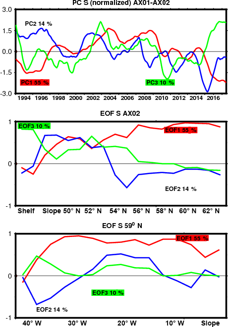
Figure 5The principal components (PCs) and spatial structure (EOFs) of an EOF analysis of salinity jointly for B-AX01 and B-AX02 (July 1993–December 2017) (we applied a 15-month running mean prior to the EOF analysis). The PCs are normalized to 1, and the EOF scaling is such that 1 indicates that the EOF explains 100 % of total local variance.
3.3 EOF analysis of interannual variability
To illustrate the potential of these binned data to investigate interannual variability, we perform EOF analysis. For this analysis, gaps in the time series are filled by first linearly interpolating from neighboring spatial bins, and then in time from neighboring time steps. They are then normalized to unit variance.
When performing an EOF analysis of the monthly anomalies of S, on B-AX01 and B-AX02 together, little seasonal dependence is observed in the first two components: very close time series are obtained when performing the EOF analysis on the whole time series or on low-passed filtered time series for different seasons (not shown). The associated principal components are very similar when performed separately for B-AX01 and B-AX02, and thus we jointly analyzed the two gridded data sets after low-pass filtering by a 15-month running mean filter (Fig. 5), to emphasize the low-frequency component of the variability. The principal components associated with EOF1 and EOF2 both present a large variability at periods of 5 years or more. The largest negative PC1 anomalies occurred in 1994–1995 and in 2016–2017, and the largest positive values in 2004 and 2009, whereas the largest negative PC2 values are in 2015, but with an apparent trend superimposed. PC1 resembles the sea surface height variability in the northern North Atlantic and hence gyre variability (Chafik et al., 2018). Both PC1 and PC2 thus have a large part of their variance at decadal or longer periods.
EOF1 has large positive values across the two sections, except in the far west of AX01 (close to the eastern Greenland Current), and on the Labrador shelf. EOF2, which overall explains only 14 % of the variance, has positive values both in the Labrador Sea (B-AX02 south of 53∘ N) and in the western Iceland Basin (27–17∘ W) along B-AX01 (to a smaller scale), with negative values in the Irminger Sea along AX01 peaking near 40∘ W. Maximum values (where it is positive) never explain more than 50 % of the local variance. EOF3 (10 % of the variance) has large values only over the Labrador shelf and slightly north of it until 55∘ N along B-AX02, and seems to correspond to higher-frequency variability.
This illustrates the potential of the binned data to investigate the low-frequency surface variability.
The gridded data set is freely available and accessible at https://doi.org/10.6096/SSS-BIN-NASG. The XBT data collected along AX01 and AX02 are available at http://www.aoml.noaa.gov/phod/hdenxbt (last access: July 2018).
ARMOR3D (GLOBAL_REP_PHY_001_021) products are freely available through the Copernicus Marine Environment Monitoring service (http://marine.copernicus.eu/services-portfolio/access-to-products/, last access: July 2018).
The International Argo Program is part of the Global Observing System (Argo, 2000).
The validated data presented here are able to characterize the seasonal variability of surface temperature and salinity along two transects crossing the North Atlantic subpolar gyre (along 59∘ N and from southwestern Iceland to southeastern Newfoundland) from July 1993 to December 2017. The time series presented here describe the interannual variability at seasonal resolution over this 21- to 25-year period except for some winter gaps over the Newfoundland shelf and along western Greenland, as well as until 1996 in the Iceland Basin along 59∘ N, and until mid 1997 along parts of western Greenland. As shown in the Appendices, to describe the seasonal to decadal surface variability, these time series are better than current SST or SSS ocean data gridded analyses such as those provided in EN4 (Good et al., 2013) or CORA (Cabanes et al., 2013; Gaillard et al., 2016), in particular before the Argo period. The time series provide added information, in particular on the shelves and continental slope regions, that is not available from Argo float data, despite Argo reaching nominal density since the early 2000s. Also, they are complementary to indirect analyses of the variability based largely on satellite altimetry (Stendardo et al., 2016), which only work as long as a strong relationship between dynamic height, sea level, and surface T and S exists, such as near fronts in the open ocean (Dong et al., 2015). This excludes most of the area investigated here.
In the interior of the subpolar gyre, the time series can be used to precisely monitor the arrival of very large freshwater salinity anomalies in recent years, and to characterize how they relate or not to temperature anomalies. They also suggest similarities to an earlier event in 1994–1996, which is unfortunately not as well sampled overall (Reverdin et al., 2002). The salinity time series are rather different on the shelves sampled here, in particular west of Greenland and near Newfoundland. This is expected, because of the different water masses with a large proportion of water advected from the Arctic or influenced by continental inputs. Sampling with the ships of opportunity is not always sufficient in these areas, due to the presence of seasonal sea ice, and would need to be complemented by other observational platforms.
In some areas, such as on the shelves or south of 54∘ N along B-AX02, there is a seasonal modulation of surface salinity variability. In most areas, salinity variability tends to be largest in summer or early autumn, although there are areas, such as along 59∘ N, with a weak seasonal cycle of this variability. Further interpretation of these data would require at least contemporary information on air–sea fluxes (heat, fresh water), mixed layer depth, and ocean circulation.
Results and data presented here highlight the importance of repeated ocean observations from volunteer ships, and the value of complementary data to better assess and monitor the state of the ocean and its variability from seasonal to interannual timescales.
TSG observations from M/V Nuka Arctica are the largest contribution to B-AX01, N-AX01 and G-AX01 since 1997. The salinity values were validated and adjusted using mostly surface water samples following Alory et al. (2015). An intake temperature measurement was used since late 2004 to adjust the temperature measurements reported by the TSG. Before that, Nuka Arctica TSG temperatures were adjusted based on comparison with nearby data, usually showing very small differences, of less than 0.1 ∘C, and often non-significantly different from 0 ∘C.
Table A1Statistical summary of the comparisons of collocated Argo data (at 3–9 m) with TSG data along AX01 and AX02 (within 58–61∘ N) (with temperature and salinity differences less than 1 ∘C and 0.2 psu, respectively) and summary of comparison of simultaneous XBT (at 7 m) and TSG temperature transects along AX01 (for each transect, the average difference is estimated, and retained if the standard deviation of the differences in individual matches is less than 0.2 ∘C). In each case, average and rms standard deviations are provided.
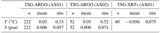
We checked the consistency of these T-S data of Nuka Arctica with other upper ocean data (Table A1). The TSG temperature and salinity data do not present significant biases with the upper level of Argo profiles, close to 5–8 m depth. The average differences (TSG-Argo) in T of 0.03 ∘C and in S of 0.006 psu are compatible with 0 at the 95 % level (based on 222 profiles within 50 km and 5 days of ship tracks, accepting differences of 1 ∘C and of 0.2 psu, which removes 11 % of outliers).
The “adjusted” temperature reported by the TSG was also compared with the temperature of the XBTs launched usually every 3 months from the Nuka Arctica since 2001 (Rossby et al., 2017). The comparison was done with XBT temperature at 7 m depth. We first average the comparisons over individual transects and estimate a mean and rms difference. Then we average these transect summaries. When removing 5 transects for which there is too large a scatter in the individual matches (rms standard deviation larger than 0.2 ∘C), the average temperature difference for 40 transects is −0.056 ∘C with an rms difference between individual transect summaries of 0.075 ∘C (if individual transects were independent and in a Gaussian distribution, this would result in a 95 % percentile range between −0.032 and −0.080 ∘C). This average difference fits with the expected near-surface temperature warm bias of XBTs for those years (Reverdin et al., 2009). The five occurrences with larger scatter fall into two categories: two in early June with weak wind and a very likely stratification near the surface in the eastern part of the section, resulting in T from the TSG higher than T from the XBT profiles at 7 m, and three where the flow rate in the TSG was very weak (in 2001–2003). With the TSG placed in the bowhead of the ship until 2005, it is unlikely that T measured during those transects would present large biases with respect to outside SST, although clearly there is a time lag and time integration of the ocean temperature in those records. Because data at large spatial scales seemed reasonable during these weak-flow instances, we retained these data in the data set, despite the likely time delay. Furthermore, including the five events does not change significantly the average bias. Thus, in summary, although there are a few anomalous individual transects, the comparisons suggest high consistency between TSG data and other validated data a few meters below the surface.
We carried out similar comparisons for TSG data along B-AX02 (since 1994), but although average results are not statistically distinguishable from the ones on AX01 (Table A1), scatter is larger (for example in comparison to Argo data, the standard deviation of the temperature differences equals 0.51 ∘C for AX02, compared to 0.33 ∘C for AX01). The comparisons are also more difficult to interpret, because of many changes in how and where the TSGs were installed on different ships during the 1994–2016 period, frequent occurrence of insufficient flow through the instrument, and also because XBT and nearby Argo data were used to adjust the TSG temperatures. Notice also that for six crossings (in July 1993 and January and April 1994, as well as in late 2016–2017), temperature was measured by the bucket method, taking care of leaving the bucket long enough in the sea and measuring T quickly (within 30 s) after retrieving the bucket. The bucket data were compared with intake temperature measurements for two crossings, suggesting small negative biases (not exceeding −0.1 ∘C), except during high wind conditions, which were not frequent. During other crossings when there were no intake temperature measurements, the temperature measurements originating from XBTs were directly associated with salinity from water samples.
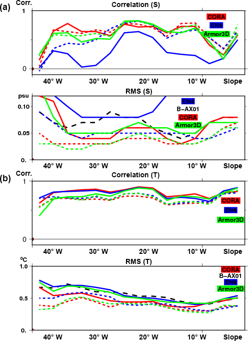
Figure B1Comparison in 1993–2015 of S and T from B-AX01 with EN4 (blue) and CORA (red) gridded data (surface, full lines; 0–500 m vertically integrated, dashed lines). Correlation coefficients are plotted, as well as the standard deviations in the different products (rms(S) and rms(T) plots; the dashed black line is for B-AX01 data). (a) is for S, and (b) is for T.
Mapped analysis products of the hydrographic data sets EN4 (Good et al., 2013; Skliris et al., 2014) and CORA (version 6.1) (Cabanes et al., 2013) are based on objective mapping, and contain a level near the surface which is used here. Mapped products from Armor3D are largely based on altimetric sea-level data with T and S adjusted to in situ T and S profiles (Guinehut et al., 2012).
We compare the binned (B-AX01) monthly time series (59–60∘ N) (Fig. 4a, c) to interpolated EN4, CORA6.1, and Armor3D products at the same sites and with additional 1–2–1 smoothing applied over successive months (EN4-AX01, CORA-AX01, Armor3D-AX01) (June 1993 to December 2015). The results are summarized by presenting longitude sections of correlation and rms variability (Fig. B1). For S, there is little correlation in SSS with EN4, except in the western Iceland Basin, and rms variability is much higher in EN4 surface fields (often by a factor of 2). Amplitudes are closer in CORA-AX01 and Armor3D-AX01, although these are smaller than those observed in the eastern Irminger Sea, and correlation is high except near the slopes. Interestingly, when averaging vertically EN4 salinity over the 0–500 m layer, correlation with B-AX01 strongly increases everywhere (with coefficients often larger than 0.6), and becomes significant and comparable to what is found for CORA-AX01 or Armor3D-AX01, except in the central and western parts of the Irminger Sea. Although this is a region where it is known that surface low-frequency variability tends to be correlated at depth (Reverdin et al., 2018), one expects a decrease in correlation between the surface and greater depths. The better correlation with vertically integrated quantities than with analysis at the same (5 m) level in EN4 suggests that “noisy” or “erroneous” data are not properly filtered in the EN4 surface analysis. It is also found that CORA analyses are more correlated vertically than EN4, which points in the same direction. To a large extent, CORA and EN4 products rely on the same data, largely on Argo (and earlier PALACE) floats as well as research cruise CTD data, whereas B-AX01 strongly relies on TSG data (to a large extent from Nuka Arctica). These mapped products differ in how they are produced. EN4 will tend to stick more to local data, whereas the CORA analysis scheme is a classical objective mapping of deviations from a guess field. Thus, it will damp variability when there are not enough data within the radius of integration (Gaillard et al., 2009). This is likely to have often been the case before the Argo float deployments in 2001–2002. Thus, CORA will underestimate the variability but be less noisy. The lack of data probably also explains the absence in this product of the low-salinity signals in 1993–1995.
For SST, the correlation of B-AX01 with all the gridded products along this zonal section is quite large (larger than 0.80 everywhere, albeit a little smaller for Armor3D), with rms variability of the same magnitude as the one in B-AX01 in the different products (although slightly smaller in CORA). The data coverage (XBTs in addition to Argo, PALACE, and CTD casts) is often quite good, with the largest differences in 1993–1996 when data coverage is weaker. Despite possible near-surface stratification, the large similarity in T between B-AX01 and EN4 suggests that the different temperature data sets are consistent. The correlation with vertically integrated temperature is smaller than at the surface and rather similar in the two products, again pointing to rather well data-constrained analyses.
The comparison of TSG data with Argo profile data (Appendix A) gives confidence in S accuracy from Nuka Arctica and thus in B-AX01 time series. Thus, the large difference in S between EN4 and B-AX01 is indicative of large seasonal noise in EN4 surface salinity, maybe resulting from insufficient sampling of meso-scale, short-term variability, in particular from Argo and other (earlier) profiling salinity floats. In the western and central Irminger Sea, the objective mapping technique used in EN4 could also spread an influence of distant data of the cold and fresh water of the eastern Greenland shelf and slope, which have very different values.
GR has contributed to the data validation and data compilation along the two ship of opportunity lines (AX01 and AX02) since the project was initiated in 1993. HV has provided support in Iceland and contributed to the scientific discussion on the data compilation. GA has been in charge of AX02 data correction and validation. DD installed the TSG on M/V Nuka Arctica in 1997 and has monitored the data since then. FB and GG at NOAA/AOML have supported the TSG and XBT operations for many years on AX02. LC has contributed to the comparison of the gridded products to EN4, and TS has contributed to the comparison of the gridded product with CORA. LH has been the contact for M/V Nuka Arctica in Nuuk (Greenland) and analyzed a large part of the water samples used for the data calibration of AX01.
The authors declare that they have no conflict of interest.
This is a contribution to the French SSS observation service, which is
supported by French agencies INSU/CNRS, IRD, CNES, and IPEV. We are very
grateful to the crews of the different vessels on lines AX01 and AX02 from
which the salinity and temperature data have been collected, in particular
under the EIMSKIP and Royal Arctic Line (RAL) managements. We acknowledge the
strong support of this operation by Lars Heilman in Nuuk, Magnus Danielsen in
Reykjavik, Hans Magnussen in Aalborg, Denis Pierrot, and Francis Bringas.
NOAA/AOML and NOAA/CPO Ocean Observing and Monitoring Division have
contributed by maintaining the TSGs along AX02 and providing XBTs on the
different ships that have operated along the AX01 and AX02 transects.
Coriolis contributed by providing XBTs to M/V Nuka Arctica and by
supporting the production of the CORA data set.
Edited by: Giuseppe M. R. Manzella
Reviewed by: two anonymous
referees
Alory, G., Delcroix, T., Téchiné, P., Diverrès, D., Varillon, D., Cravatte, S., Gouriou, Y., Grelet, J., Jacquin, S., Kestenare, E., Maes, C., Morrow, R., Perrier, J., Reverdin, G., and Roubaud, F.: The French contribution to the Violuntary Observing Ships Network of Sea Surface Salinity, Deep-Sea Res. Pt. I, 105, 1–18, https://doi.org/10.1016/j.DSR.2015.08.005, 2015.
Argo: Argo float data and metadata from Global Data Assembly Centre (Argo GDAC), SEANOE, https://doi.org/10.17882/42182, 2000.
Bojariu, R. and Reverdin, G.: Large-scale variability modes of freshwater flux and precipitation over the Atlantic, Clim. Dynam., 18, 369–381, 2002.
Böning, C. W., Behrens, E., Biastoch, A., Getzlaff, K., and Bamber, J. L.: Emerging Impact of Greenland Meltwater on Deepwater Formation in the North Atlantic Ocean, Nat. Geosci., 9, 523–527 https://doi.org/10.1038/ngeo2740, 2016.
Cabanes, C., Grouazel, A., von Schuckmann, K., Hamon, M., Turpin, V., Coatanoan, C., Paris, F., Guinehut, S., Boone, C., Ferry, N., de Boyer Montégut, C., Carval, T., Reverdin, G., Pouliquen, S., and Le Traon, P.-Y.: The CORA dataset: validation and diagnostics of in-situ ocean temperature and salinity measurements, Ocean Sci., 9, 1–18, https://doi.org/10.5194/os-9-1-2013, 2013.
Cayan, D. R.: Latent and sensible heat flux anomalies over the northern oceans: driving the sea surface temperature, J. Phys. Oceanogr., 22, 859–881, 1992.
Chafik, L., Rossby, T., and Schrum, C.: On the spatial structure and temporal variability of poleward transport between Scotland and Greenland, J. Geophys. Res., 119, 824–841, https://doi.org/10.1002/2013JC009287, 2014.
Chafik, L., Nilsen, J. E. Ø., Dangendorf S., Reverdin, G., and Frederikse, T.: North Atlantic Ocean Circulation and Decadal Sea 1 Level Change During the Altimetry Era, in preparation, 2018.
Davis, R. E., Sherman, J. T., and Dufour, J.: Profiling ALACEs and other advances in autonomous subsurface floats, J. Atmos. Ocean. Tech., 18, 982–993, 2001.
De Jong, M. F. and de Steur, L.: Strong winter cooling over the Irminger Sea in winter 2014–2015, exceptional deep convection, and the emergence of anomalously low SST, Geophys. Res. Lett., 42, 7106–7113, https://doi.org/10.1002/2016GL069596, 2016.
Dong, S., Goni, G., and Bringas, F.: Temporal variability of the South Atlantic Meridional Overturning Circulation between 20 ∘S and 35 ∘S, Geophys. Res. Lett., 42, 7655–7662, https://doi.org/10.1002/2015GL065603, 2015.
Fettweis, X., Box, J. E., Agosta, C., Amory, C., Kittel, C., Lang, C., van As, D., Machguth, H., and Gallée, H.: Reconstructions of the 1900–2015 Greenland ice sheet surface mass balance using the regional climate MAR model, The Cryosphere, 11, 1015–1033, https://doi.org/10.5194/tc-11-1015-2017, 2017.
Foukal, N. P. and Lozier, M. S.: Assessing variability in the size and strength of the North Atlantic subpolar gyre, J. Geophys. Res.-Oceans, 122, 6295–6308, https://doi.org/10.1002/2017JC012798, 2017.
Friedman, A. R., Reverdin, G., Khodri, M., and Gastineau, G.: A new record of Atlantic sea surface salinity from 1896 to 2013 reveals the signatures of climate variability and long-term trends, Geophys. Res. Lett., 44, 1866–1876, https://doi.org/10.1002/2017GL072582, 2017.
Fröb, F., Olsen, A., Vage, K., Moore, G. W., Yashayaev, I., Jeansson, E., and Rajasakaren, B.: Irminger Sea deep convection injects oxygen and anthropogenic carbon to the ocean interior, Nat. Commun., 7, 13244, https://doi.org/10.1038/ncomms13244, 2016.
Gaillard, F., Autret, E., Thierry, V., Galaup, P., Coatanoan, C., and Loubrieu, T.: Quality control of large Argo datasets, J. Atmos. Ocean. Tech., 26, 337–351, 2009.
Gaillard, F., Reynaud, T., and Thierry, V.: In Situ-Based Reanalysis of the Global Ocean Temperature and Salinity with ISAS: Variability of the Heat Content and Steric Height, J. Clim., 29, 1305–1323, https://doi.org/10.1175/JCLI-D-15-0028.1, 2016.
Good, S. A., Martin, M. J., and Rayner, N. A.: EN4: quality controlled ocean temperature and salinity profiles and monthly objective analyses with uncertainty estimates, J. Geophys. Res., 118, 6704–6716, 2013.
Guinehut, S., Dhomps, A.-L., Larnicol, G., and Le Traon, P.-Y.: High resolution 3-D temperature and salinity fields derived from in situ and satellite observations, Ocean Sci., 8, 845–857, https://doi.org/10.5194/os-8-845-2012, 2012.
Häkkinen, S., Rhines, P. B., and Worthen, D. L.: Atmospheric blocking and Atlantic multidecadal ocean variability, Science, 334, 655–659, https://doi.org/10.1126/science.1205683, 2011.
Häkkinen, S., Rhines, P. B., and Worthen, D. L.: Northern North Atlantic sea surface height and ocean heat content variability, J. Geophys. Res., 118, 3670–3678, https://doi.org/10.1002/jgrc.20268, 2013.
Hatun, H., Sando, A. B., Drange, H., Hansen, B., and Valdimarsson, H.: Influence of the Atlantic subpolar gyre on the thermohaline circulation, Science, 309, 1841–1844, 2005.
Holliday, N. P., Cunningham, S. A., Johnson, C., Gary, S. F., Griffiths, C., Read, J. F., and Sherwin, T.: Multidecadal variability of potential temperature, salinity, and transport in the eastern subpolar North Atlantic, J. Geophys. Res., 120, 5945–597, https://doi.org/10.1002/2015JC010762, 2015.
Hurrell, J. W., Kushnir, Y., Ottersen, G., and Visbeck, M.: An overview of the North Atlantic Oscillation: climate significance and Environmental impact, Geophys. Monogr. Ser., American Geophysical Union, https://doi.org/10.1029/GM134, 2013.
Josey, S. A. and Marsh, R.: Surface freshwater flux variability and recent freshening of the North Atlantic in the eastern subpolar gyre. J. Geophys. Res., 110, C05008, https://doi.org/10.1029/2004JC002521, 2005.
Josey, S., Hirschi, J. J.-M., Sinha, B., Duchez, A., Grist, J. P., and Marsh, R.: The recent Atlantic cold anomaly: causes, consequences and related phenomena, Ann. Rev. Mar. Sci., 10, 475–501, https://doi.org/10.1146/annurev-marine-121916-063102, 2017.
Kennedy, J. J., Rayner, N. A., Smith, R. O., Parker, D. E., and Saunby, M.: Reassessing Biases and Other Uncertainties in Sea Surface Temperature Observations Measured in Situ since 1850: 1. Measurement and Sampling Uncertainties, J. Geophys. Res., 116, D14103, https://doi.org/10.1029/2010JD015218, 2011a.
Kennedy, J. J., Rayner, N. A., Smith, R. O., Saunby, M., and Parker, D. E.: Reassessing biases and other uncertainties in sea-surface temperature observations since 1850: 2. Biases and homogenisation, J. Geophys. Res., 116, D14104, https://doi.org/10.1029/2010JD015220, 2011b.
Kolodziejczyk, N., Prigent-Mazella, A., and Gaillard, F.: ISAS-15 temperature and salinity gridded fields, SEANOE, https://doi.org/10.17882/52367, 2017.
Lavender, K. L., Davis, R. E., and Owens, W. B.: Mid-depth recirculation observed on the interior Labrador and Irminger seas by direct velocity measurements, Nature, 607, 66–69, 2000.
Piecuch, C., Ponte, R. M., Little, C. M., Buckley, M. W., and Fukumori, I.: Mechanisms underlying recent changes in subpolar North Atlantic Ocean heat content, J. Geophys. Res., 122, 7181–7197, https://doi.org/10.1002/2017JC012845, 2017.
Piron, A., Thierry, V., Mercier, H., and Caniaux, G.: Gyre-scale deep convection in the subpolar North Atlantic Ocean during winter 2014–2015, Geophys. Res. Lett., 44, 1439–1447, https://doi.org/10.1002/2016GL071895, 2017.
Rahmstorf, S., Box, J. E., Feulner, G., Mann, M. E., Robinson, A., Rutherford, S., and Schaffernicht, E. J.: Exceptional twentieth-century slowdown in Atlantic Ocean overturning circulation, Nat. Clim. Change, 5, 475–480, https://doi.org/10.1038/nclimate2554, 2015.
Reverdin, G., Durand, F., Mortensen, J., Schott, F., Valdimarsson, H., and Zenk, W.: Recent changes in the surface salinity of the North Atlantic subpolar gyre, J. Geophys. Res., 107, 8010, https://doi.org/10.1029/2001JC001010, 2002.
Robson, J., Ortega, P., and Sutton, R.: A reversal of climate trends in the North Atlantic since 2005, Nat. Geosci., 9, 513–517, https://doi.org/10.1038/ngeo2727, 2016.
Rossby, T., Reverdin, G., Chafik, L., and Soiland, H.: A direct estimate of poleward volume, heat, and freshwater fluxes at 59.5∘ N between Greenland and Scotland, J. Geophys. Res., 122, 5870–5887, https://doi.org/10.1002/2017JC012835, 2017.
Sarafonov, A.: On the effect of the North Atlantic Oscillation on temperature and salinity of the subpolar North Atlantic intermediate and deep waters, ICES J. Mar. Sci., 66, 1448–1454, 2009.
Skliris, N., Marsh, R., Josey, S. A., Good, S. A., Liu, C., and Allan, R. P.: Salinity changes in the World Ocean since 1950 in relation to changing surface freshwater fluxes, Clim. Dynam., 43, 709–736, https://doi.org/10.1007/s00382-014-2131-7, 2014.
Stendardo, L., Rhein, M., and Hollmann, R.: A high resolution salinity time series 1993–2012 in the North Atlantic from Argo and altimeter data, J. Geophys. Res., 121, 2523–2551, https://doi.org/10.1002/2015JC011439, 2016.
Thierry, V., de Boisséson, E., and Mercier, H.: Interannual variability of the subpolar mode water properties over the Reykjanes Ridge, J. Geophys. Res., 113, C04016, https://doi.org/10.1029/2007JC004443, 2008.
van den Broeke, M. R., Enderlin, E. M., Howat, I. M., Kuipers Munneke, P., Noël, B. P. Y., van de Berg, W. J., van Meijgaard, E., and Wouters, B.: On the recent contribution of the Greenland ice sheet to sea level change, The Cryosphere, 10, 1933–1946, https://doi.org/10.5194/tc-10-1933-2016, 2016.
Yashayaev, I. and Loder, J. W.: Recurrent replenishment of Labrador Sea water and associated decadal-scale variability, J. Geophys. Res., 121, 8095–8114, https://doi.org/10.1002/2016JC012046, 2016.
Zunino, P., Lherminier, P., Mercier, H., Daniault, N., García-Ibáñez, M. I., and Pérez, F. F.: The GEOVIDE cruise in May–June 2014 reveals an intense Meridional Overturning Circulation over a cold and fresh subpolar North Atlantic, Biogeosciences, 14, 5323–5342, https://doi.org/10.5194/bg-14-5323-2017, 2017.