the Creative Commons Attribution 4.0 License.
the Creative Commons Attribution 4.0 License.
 | 15 Nov 2018
A 40-year global data set of visible-channel remote-sensing reflectances and coccolithophore bloom occurrence derived from the Advanced Very High Resolution Radiometer catalogue
Benjamin Roger Loveday
Timothy Smyth
A consistently calibrated 40-year-long data set of visible-channel remote-sensing reflectance has been derived from the Advanced Very High Resolution Radiometer (AVHRR) sensor global time series. The data set uses as its source the Pathfinder Atmospheres – Extended (PATMOS-x) v5.3 Climate Data Record for top-of-atmosphere (TOA) visible-channel reflectances. This paper describes the theoretical basis for the atmospheric correction procedure and its subsequent implementation, including the necessary ancillary data files used and quality flags applied, in order to determine remote-sensing reflectance. The resulting data set is produced at daily, and archived at monthly, resolution, on a grid at https://doi.org/10.1594/PANGAEA.892175. The primary aim of deriving this data set is to highlight regions of the global ocean affected by highly reflective blooms of the coccolithophorid Emiliania huxleyi (where lith concentration >2–5×10⁴ mL−1) over the past 40 years.


Remote-sensing reflectance (Rrs), which has been listed as an Essential Climate Variable by the Global Climate Observation System, has been routinely monitored at the global scale by ocean colour satellites since the launch of the Sea-Viewing Wide Field-of-view Sensor (SeaWiFS) in September 1997. Prior to this, the proof-of-concept Coastal Zone Color Scanner (CZCS) provided sporadic coverage for the period 1978–1986. Spectral Rrs is a primary measurement of ocean colour satellites and is used to determine higher-level products such as inherent optical properties (Smyth et al., 2006), chlorophyll a (O'Reilly et al., 1998) and particulate inorganic carbon (Balch et al., 2005). Rrs can also be used directly to detect brighter areas of the ocean caused by large blooms of the coccolithophorid Emiliania huxleyi, as they shed highly backscattering calcium carbonate “liths” into the surrounding waters.
A subjective analysis, visually comparing global maps of coccolithophorid blooms during the CZCS era (Plate 1 from Brown and Yoder, 1994) and the first few years of the SeaWiFS mission (Fig. 1 from Iglesias-Rodriguez et al., 2002), clearly shows large distributional changes in bloom occurrence between the two periods (Winter et al., 2013). However, the two analyses are separated by a decade where no ocean colour sensors were in operation. In the 1980s, Groom and Holligan (1987) published a coccolithophorid bloom algorithm for use on visible-channel Advanced Very-High Resolution Radiometer (AVHRR) data. The potential for using the AVHRR series of satellites, which spans the period between 1978 and the present, as a means for bridging the observational gap between CZCS and SeaWiFS was seized upon by several studies (Morozov et al., 2013) with a particular emphasis on high-latitude seas (Merico et al., 2003; Smyth et al., 2004). This built upon work in the 1980s and 1990s, before the observational hiatus became an issue (Ackleson and Holligan, 1989; Matrai and Keller, 1993; Holligan et al., 1993; Garcia-Soto et al., 1995) and despite lower inherent reflectances in AVHRR channel 1 (0.580–0.680 µm) and lower detector gain rendering the sensor only 11 % as sensitive to variation in coccolithophore reflectance as CZCS channel 3 (0.540–0.560 µm) (Groom and Holligan, 1987).
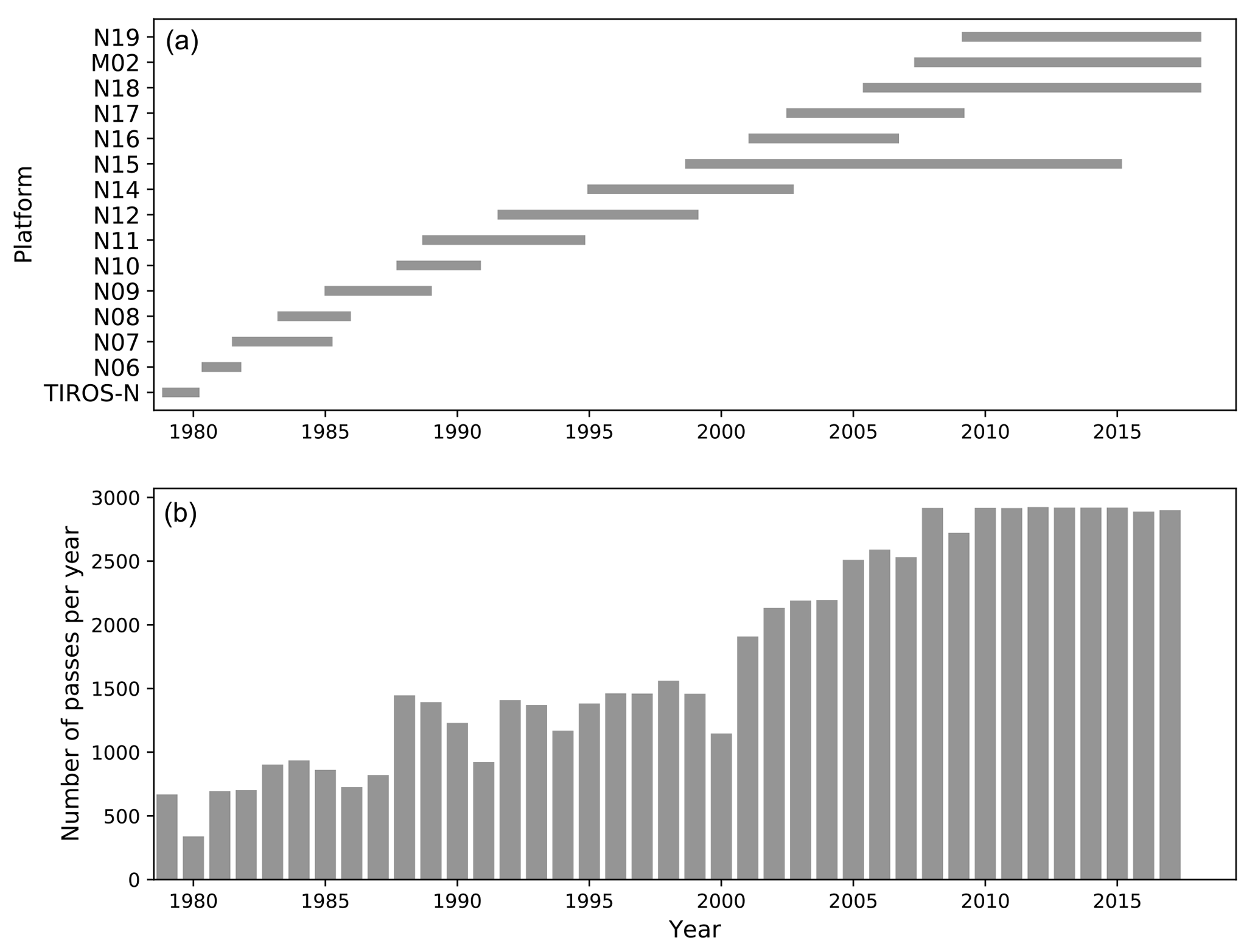
Figure 1PATMOS-x v5.3 (Px5.3) data density. (a) The length of the individual AVHRR missions: TIROS-N (the NASA-operated Television Infra-Red Observation Satellite); NOAA-operated missions (N); and MetOp (M) missions operated by EUMETSAT. (b) Number of satellite orbits per year which comprise the Px5.3 data set.
More recently, Uz et al. (2013) used the inter-calibrated AVHRR reflectances provided by the Clouds from AVHRR Extended (CLAVR-x) project (Heidinger et al., 2002) to produce a global 25-year global record of coccolithophorid blooms at 0.25∘ resolution. This study suggested a long-term decline in the bloom surface area, correlated with warming sea surface temperature and increased mixed-layer depth. However, CLAVR-x processor is not optimised for climate studies, and the 25-year time period of the resulting analysis was, at the time, not long enough to assess bloom sensitivity to decadal climate modes. Subsequently, the CLAVR-x processor was optimised for climate studies as part of the the Pathfinder Atmospheres – Extended (PATMOS-x) project.
PATMOS-x (Heidinger et al., 2014) provides a new suite of climate data records that include cloud brightness, aerosol properties and top-of-atmosphere (TOA) reflectances, derived from the continuous ∼40-year global AVHRR catalogue. Crucially, these quantities are optimised for climate studies and have consistently calibrated reflectances across sensors, and the products are geolocated on a 0.1∘ grid: an order of magnitude finer than the data used in previous CLAVR-x-based coccolithophorid studies. Further information on the data set is available at https://cimss.ssec.wisc.edu/patmosx/ (last access: 14 November 2018).
In this paper we describe the exploitation of the PATMOS-x output to derive a new data set, which comprises a daily global Rrs product and an associated coccolithophorid bloom map. By adopting this approach, the current time period over which quantitative analyses of global Rrs can be carried out will be doubled from 20 to nearly 40 years. It is over this order of observational time period that climatic shifts have been shown to be demonstrable (Henson et al., 2010).
Previous efforts to derive visible-channel Rrs from the AVHRR catalogue (e.g. Groom and Holligan, 1987; Smyth et al., 2004) typically use the raw instrument counts as a starting point to calculate per-channel TOA radiance. In order to apply this approach across the lifetime of a single AVHRR sensor, the radiance must be calibrated according to the sensor degradation parameters. However, as sensor degradation parameters are only available for AVHRR sensors on NOAA-7, 9, 11 and 14 (Rao and Chen, 1995, 1996), the approach is not applicable for analysis of long-term global signals. Consequently, here we adopt a modified version of the approach used by Groom and Holligan (1987), and updated by Smyth et al. (2004), which uses the TOA reflectances as a starting point for the atmospheric correction procedure. The approach is fully detailed in Sect. 3.1.3.
Per-channel TOA reflectances are extracted directly from version 5.3 of the PATMOS-x data set (Heidinger et al., 2014) (available at https://doi.org/10.7289/V56W982J and subsequently referred to here as Px5.3). Px5.3 reflectances are inter-calibrated across AVHRR sensors and are corrected for sensor degradation throughout. Px5.3 is the first consistently gridded, climate quality data record of cross-calibrated AVHRR reflectances. It spans the period from 1979 to the present and contains between 2 and 10 passes per day, dependent on the number of AVHRR instruments operational on the TIROS-N, NOAA and MetOp platforms at the time (Fig. 1). The Rrs data set derived from this record spans from 1979 to 2017 and includes the analysis of 62 359 orbits. To calculate Rrs, we use the visible channel 1 (0.63 µm, 0.1 µm bandwidth) and the near infra-red (NIR) channel 2 (0.86 µm, 0.275 µm bandwidth) data. Channel 2 is predominantly used to correct for atmospheric aerosol effects, as the ocean is assumed to be dark in the NIR (e.g. Rrs=0).
To facilitate the atmospheric correction scheme, cloud cover, water vapour and trace gas concentrations, winds, mean sea level pressure and sea surface temperature fields are extracted from the gridded, 6-hourly ERA-Interim products, provided by the European Centre for Medium-Range Weather Forecasts (ECMWF) (available via https://www.ecmwf.int/en/forecasts/datasets/reanalysis-datasets/era-interim, last access: 14 November 2018).
3.1 Processing chain
Figure 2 presents a schematic diagram of the processing chain used to derive the Rrs and the associated coccolithophorid bloom map. The processor initial stages (Sect. 3.1.1–Sect. 3.1.4) are applied to each image in turn. The images are then aggregated into daily composites and monthly climatologies. Each stage of the processor is sequentially discussed below.
3.1.1 Initial quality control (QC1)
To prevent the calculation of erroneous Rrs values, input reflectance data are masked according to a series of criteria based on measurement fidelity and consideration of the appropriate flags. The QC1 processor only retains reflectances where the following conditions are met:
-
the cloud mask is equal to 0 (clear conditions),
-
the glint mask is equal to 0 (no glint present),
-
the land mask is not equal to 1 (permitting only ocean, coastal and inland water pixels),
-
the “bad pixel” mask is equal to 0,
-
the snow class mask is equal to 0 (no sea ice),
-
is satisfied for both channel 1 and channel 2,
-
the sensor and solar zenith angles are finite and <90∘,
-
the relative azimuth angle is finite.
Once these masking operations are complete, the QC1 processor passes the quality-controlled TOA reflectances to the Rrs processor, which awaits atmospheric inputs.
3.1.2 Atmospheric processor
Atmospheric data are required to calculate both the contribution of whitecaps to the ocean reflectance and the gas absorbance transmission scaling factors for ozone and water vapour. For each scene, the atmospheric processor bilinearly interpolates the contemporaneous ERA-Interim fields onto the Px5.3 grid, in both space and time. Wind speed at 10 m (m s−1), ozone concentration (Dobson units) and water vapour concentration (kg m−2) are passed to the Rrs processor to support atmospheric correction.
3.1.3 Rrs processor: atmospheric correction
The total TOA radiance measured by a satellite contains contributions from atmospheric scattering, reflections from the sea surface and the water-leaving radiance. The water-leaving component is of primary interest here and is typically much smaller than the atmospheric signal. Consequently, we must perform an atmospheric correction procedure to isolate the signal of interest.
In general terms, the TOA radiance can be written as (Franz et al., 2007)
where LTOA, LRayl, LA, Lwcap and Lw refer to the radiance (L) at the top of atmosphere, due to Rayleigh scattering, due to aerosol scattering, due to whitecaps and due to the water-leaving components, respectively. The transmission coefficients for atmospheric gases (tg) and the associated atmospheric scaling factors (td) are superscripted according to the solar (0) and sensor (s) viewing directions. AVHRR is minimally sensitive to changes in polarisation (Zhao et al., 2004), and the polarisation factor, fp, is set to unity.
P5.3x provides calibrated TOA bi-directional reflectance which has been normalised by , where F0 is the solar constant (Neckel and Labs, 1984), R∕R0 the Earth–Sun distance ratio and θ0 the solar zenith angle. Therefore, it is convenient to recast Eq. (1) in terms of reflectance. As remote-sensing reflectance (Rrs) is defined as the water-leaving radiance (Lw) divided by the downwelling irradiance (Ed), and Ed is proportional to the incoming solar radiance (as shown in Eq. 2), Eq. (1) can be re-written as Eq. (3).
where Rn is the corrected reflectance for the given channel, denoted by the n subscript. As the first bracketed term in Eq. (3) is proportional to the TOA reflectance provided by the P5.3x data set, Eq. (3) can be re-written as
where , and are the channel n Rayleigh, whitecap and aerosol reflectance terms, respectively. Each of these correction terms are now discussed in turn.

Figure 2Schematic diagram showing the different stages of the remote-sensing reflectance (Rrs) processing chain. The blue-shaded region generates the unfiltered Rrs product; the red-shaded region subsequently generates the filtered Rrs product. PML, NOAA and ECMWF refer to Plymouth Marine Laboratory, the National Oceanic and Atmospheric Administration and the European Centre for Medium-Range Weather Forecasts, respectively.
Rayleigh scattering is a function of wavelength, and satellite and solar-viewing angles. For each wavelength, the Rayleigh reflectance, , is bilinearly interpolated from a look-up table of Rayleigh radiance components, discretised by 2∘ solar and satellite zenith angles and normalised by the extraterrestrial solar irradiance (Neckel and Labs, 1984). The look-up table was calculated using values of 0.057 and 0.02 for the Rayleigh scattering optical depth (τ) for the AVHRR visible and NIR channels, respectively (Elterman, 1970). Each entry in the table contains three sets of Rayleigh radiance components, , and total Rayleigh reflectance is calculated using
where A0(λ), A1(λ) and A2(λ) are the linearly interpolated Rayleigh radiances for a given wavelength, solar zenith angle and relative azimuth (), where θs is the satellite zenith angle.
Reflectance due to whitecaps is a function of both wind speed and wavelength. Here, this is calculated according to the method described by Koepke (1984). The whitecap reflectance is calculated using
where λ is wavelength in microns; U10 is the 10 m wind speed, as provided by the ingested ERA interim fields; and R(λ)ef is the wavelength-dependent effective reflectance. The appropriate effective reflectance value is interpolated from a look-up table derived from Koepke (1984), generalised to include NIR wavelengths.
To correct for aerosol effects, we adopt the approach used by Smyth et al. (2004) and Uz et al. (2013). The assumptions here are twofold: firstly that the aerosol reflectance for channel 1 and channel 2 is equal (Stumpf and Pennock, 1989) and secondly that Rrs in channel 2 is zero. Using these assumptions, the reflectances in the visible and NIR channels can be used to isolate and remove the aerosol signal from the reflectance calculation, using Eq. (7):
where pl is the atmospheric path length () and τ0 is the Rayleigh optical depth for channel 1 for a path length of unity. R1 and R2 are the respective channel 1 and 2 TOA reflectances (RTOA), corrected for Rayleigh scattering (RRayl), whitecaps (Rwcap) and atmospheric transmission (as given by Eq. 4). Rrs values are not retained where the Rayleigh reflectance calculation fails.
Ozone and water vapour absorption values for AVHRR channels 1 and 2 are provided by Liang (2005) and Tanre et al. (1992), and implemented as
where the ozone and water vapour transmission components along the sensor viewing path length are calculated according to equations of the form
B0(λ) and B1(λ) are the wavelength-dependent absorption coefficients for each channel and gas. Concentration values for ozone [O3], and for water vapour [H2O], are interpolated from daily ERA-Interim fields. Equations (8) and (9) are similarly constructed for the solar-viewing path length. NO2 and CO2 scaling factors are set to one as their absorption is assumed to be negligible (see Liang, 2005, Fig. 2.10). Atmospheric scaling factors for each viewing path are calculated, using Eq. (10), where τR(λ) is the Rayleigh optical scattering depth.
Sunglint is explicitly flagged in and removed from the Px5.3 data sets, and no further correction for sunglint is applied.
3.1.4 Secondary quality control (QC2)
A secondary quality control procedure removes poor-quality retrievals from the calculated Rrs product, discarding pixels with negative Rrs values. Whilst a rare occurrence, Rrs pixels are also discarded where there is no acquisition time stamp as this renders the calculated Rayleigh characteristics invalid. In this case, data within a two-pixel radius of the erroneous point(s) are also discarded.
Periodically, low-quality AVHRR data give rise to patterns of erroneously high Rrs values. Typically these aberrations affect a single pass, resulting in a poor-quality “stripe” across the Rrs image. To remove this effect, each pass in the Rrs product is binned according to its integer hour of acquisition, which roughly corresponds to an individual pass (no specific pass number is available in the Px5.3 data). If a pass contains more than 5000 valid data points and has a mean Rrs value of higher than 0.001, the pass is considered to be of poor quality and all data contained within it are discarded.
Over the South Atlantic, the Earth's Van Allen belt comes close to the planet's surface. The resulting excess radiation, the so-called “South Atlantic Anomaly”, causes erroneous speckling of the AVHRR visible channel (Casadio and Arino, 2011). To remove this effect, each Rrs product is subject to a filter, which removes pixels if they have a value that is greater than 5 times the maximum value of any of its neighbours. Coherent signals, associated with blooms, are unaffected. This process also removes single isolated pixels that are surrounded entirely by bad data.
When the solar zenith angle approaches 90∘, the number of counts in the visible channel drops substantially, degrading the quality of Rrs estimate produced. To combat this effect, pixels where the number of counts in channel 1 is less than 10 are masked.
Once the final Rrs is calculated, it is written to an intermediate netCDF4 file during the “scene output” stage. The pass-by-pass Rrs product is not made available in this data set.
3.1.5 Compositing
For each day, the Rrs products, calculated for each pixel on a pass-by-pass basis, are averaged into a single daily, global product. A daily product contains the average of between 2 and 10 passes, depending on the number of AVHRR sensors in operation. Values recorded as missing or filled values in the individual netCDF4 products are masked, and are therefore not included in the averaging process. In parallel, each pass is contributed to the total aggregator stage, which calculates climatological monthly mean Rrs values for each month, along with standard deviations and the number of observations available. Analogous statistics are also calculated for the total record. The total aggregator stage can only be completed once all processed passes are available. Filtering for blooms cannot begin until the aggregator has finished constructing the climatology. The final unmasked, unfiltered Rrs product is written into a daily composite netCDF4 file as remote_sensing_reflectance, along with the original coordinate variables, as derived from the Px5.3 grid.
3.2 Filtering, masking and identifying blooms
In previous ocean-colour-based analyses, coccolithophorid bloom maps are produced as the binary classified output of a supervised multi-spectral algorithm (e.g. Iglesias-Rodriguez et al., 2002; Brown and Yoder, 1994). In this work, the availability of only one visible channel necessitates an alternative method, and the bloom map is instead produced through temporal filtering of the Rrs product, followed by selective masking to subsequently remove false positives.
Temporal filtering of the Rrs product is performed through a comparison of each daily composite to the relevant monthly mean climatological Rrs field (produced by the total aggregator stage). Rrs signals are only classified as blooms where the per-pixel Rrs value is greater than 2 monthly standard deviations above the corresponding monthly mean value. The standard deviation in this case is calculated from the monthly mean products across the entire archive. Pixels that do not match this criterion are assumed to contribute to the background, rather than bloom signal, and are therefore set to zero. The filtered bloom product, written into the daily netCDF4 file as filtered_remote_sensing_product, is then subject to further quality controls in the masking stage, as described below.
High Rrs values, while potentially indicative of coccolithophore blooms, can also occur in regions that are subject to high concentrations of suspended sediment (e.g. estuaries), or where shallow bathymetry and clear water coincide (e.g. shelf regions in oligotrophic areas). To remove these, and other false positives, the final bloom product is derived from the filtered bloom product by subjecting the latter to a number of screening processes, as detailed below.
Firstly, to remove the effects of land contamination, the bloom map is set to zero in all points within three pixels of the land mask. Secondly, following Iglesias-Rodriguez et al. (2002), the bloom map is set to zero in areas between 47∘ N and 47∘ S where the bathymetry is shallower than 100 m. This removes false positives associated with the sea floor, an effect that is most noticeable in the Caribbean and Arafura seas. Thirdly, whilst flagged sea ice has been explicitly removed from the Px5.3 data (see Sect. 3.1.1), this does not comprehensively remove ice effects. As a result of missed flagging, and of glacial (Broerse et al., 2003) and river run-off, sporadic high Rrs values that are not indicative of blooms still occur at high latitudes. To correct for this, bloom map pixels are set to zero where Rrs≥0.05 (a value far above that which we would expect in water types associated with coccolithophorid blooms). Furthermore, the Rrs product is screened using sea surface temperature (SST) data obtained from contemporaneous ERA-Interim fields, and Rrs is set to zero in pixels where SST <0 ∘C in the Northern Hemisphere, a value at which the coccolithophorid growth rate drops to near zero, even for cold-water strains such as E. huxleyi (Buitenhuis et al., 2008). Finally, bloom map pixels are set to zero where the total aggregated mean value Rrs is greater than 0.0005, removing the effects of consistent river outflows (e.g. the Amazon and around the Yellow Sea).
The final product suite is annotated with relevant metadata to ensure CF1.8 compliance, completing the processing. The contents of the data file are described fully in the following section.
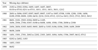
The complete finalised data set consists of 13 932 daily files, beginning 1 January 1979 and ending 31 December 2017. Table 1 describes periods where data are missing, due either to a lack of available AVHRR data in the Px5.3 archive or to a lack of viable data for Rrs processing. Completely empty scenes are not included in the archive.
Table 1Inventory of missing Rrs products in the processed archive due to missing or unviable AVHRR data.
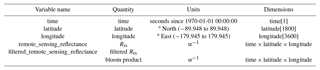
The products are provided at 0.1∘ resolution (consistent with the original Px5.3 grid). Each data file contains the variables listed in Table 2.
Responsibility for maintaining the data set lies with Plymouth Marine Laboratory, the provenance authority for the final output (Fig. 2). The data set will be updated periodically, but no specific update schedule is set. The initial release version is v1.0. Minor version updates to bring the archive up to date will increment the decimal value. Major updates in the case of changes to processing will increment the integer value.
Due to the size of the entire daily-resolution record (>60 Gb in total), the data are archived on a 1-monthly basis, with monthly mean and maximum fields available as separate files. The data set is stored in the PANGAEA archive and has the following digital object identifier: https://doi.org/10.1594/PANGAEA.892175.
5.1 Regional comparisons
Figure 3 shows a comparison between four coccolithophorid blooms detected by ocean colour sensors and the corresponding blooms in the filtered_remote_sensing_reflectance product. In all four cases where bright blooms are detected in the ocean colour sensor observations (Fig. 3a SeaWiFS; Fig. 3c, MERIS; Fig. 3e, g, MODIS) there are spatially corresponding bright patches in the AVHRR imagery. In the MERIS and MODIS cases the AVHRR imagery is from the same day (i.e. on a single overpass basis). In the SeaWiFS case, a 3-day AVHRR composite mean is used, due to differences in cloud cover at the various acquisition times, lowering the intensity of the visible bloom but preserving the spatial coverage of the scene.
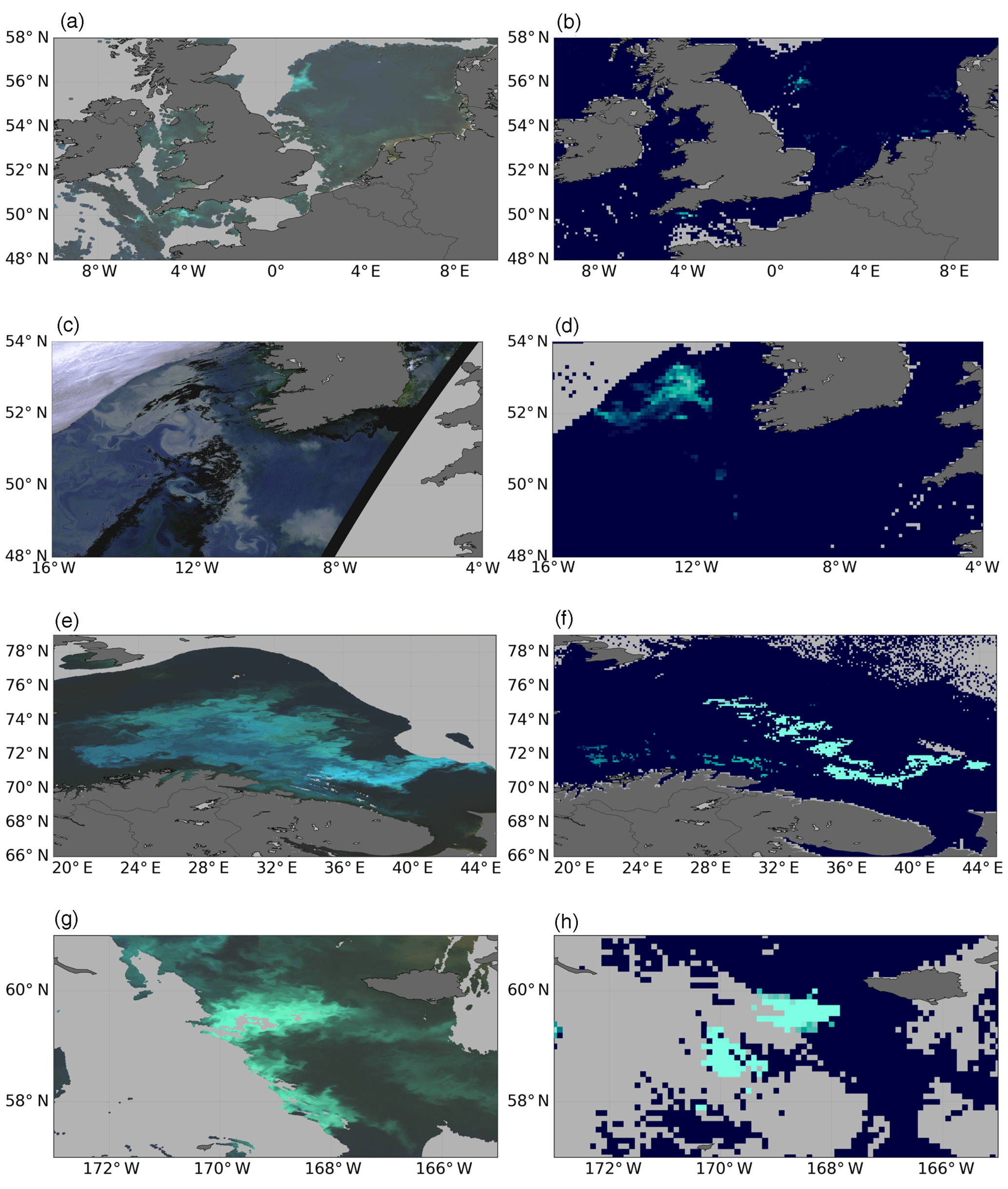
Figure 3Examples of ocean-colour-derived red–green–blue (RGB) images of coccolithophore blooms matched to their filtered bloom product counterparts. Panels are as follows. (a, c, e, g) Level 2 RGB images for the North Sea and English Channel (SeaWIFS; 30 July 1999), North Atlantic and Irish Sea (MERIS; 23 May 2010), Barents Sea (MODIS; 17 August 2011) and Bering Sea (MODIS; 4 September 2014). (b, d, f, h) Matching, contemporaneous filtered bloom product composite for each location and date. Dark grey indicates land, and light grey indicates cloud, throughout. For bloom products, dark blue indicates that no bloom is present; lighter cyan colours indicate that a bloom is present.
There is also evidence from in situ data in the English Channel case (Fig. 3a and b) that this was indeed a bloom of Emiliania huxleyi from cell counts and in-water radiometry (Smyth et al., 2002). The northern North Sea feature centred on 56∘ N, 1.5∘ E in Fig. 3a is possibly the remnants of a bloom which was the subject of an intensive field campaign during June 1999 (Burkill et al., 2002). Similarly blooms have been documented in the literature in the Barents Sea (Fig. 3e and f) which are comparable in timing and extent with some limited in situ samples (Smyth et al., 2004); Merico et al. (2003) report on blooms in the Bering Sea of similar timing and extent to those shown in Fig. 3g and h.
It is notable that the cloud (and ice) masking algorithms for the ocean colour and AVHRR sensors are in close agreement for the individual scenes shown in Fig. 3c and d, e and f, and g and h. The discrepancy in the cloud flagging for the SeaWiFS case occurs as a result of the 3-day compositing.
5.2 Global signals
Figure 4 shows the global spatial coverage of the data set, presented as decadal means of the filtered Rrs bloom product for four decadal periods. Comparing Fig. 4a with the CZCS era (1978–1986) coccolithophorid bloom map produced by Brown and Yoder (1994) suggests that the bloom signals in the North Atlantic, North Sea and Norwegian Sea and on the Argentinian coast are well captured. The presence of blooms in the Black Sea and sporadically throughout the Mediterranean is also consistent between the two. However, due to the coastal masking, the high signals around Newfoundland are not captured here. In addition, no signals are detected in the Arafura Sea or within the Indonesian archipelago, as these areas have been specifically masked due to shallow bathymetry. The signals along the coast of Greenland and in the Southern Ocean are stronger than anticipated, likely due to some remaining influence of ice and glacial river outflow.
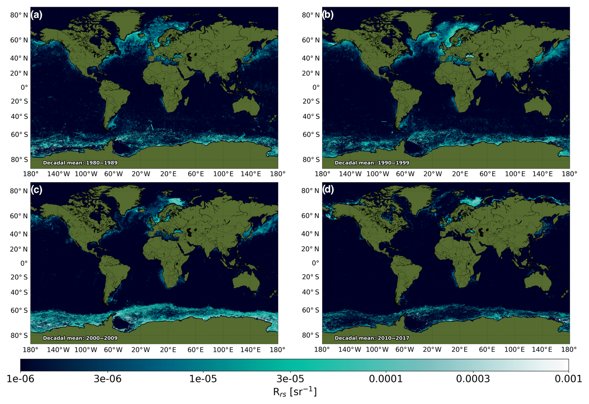
Figure 4Mean values for the filtered remote-sensing reflectance (Rrs) bloom product by decade for the (a) 1980 to 1989, (b) 1990–1999, (c) 2000–2009 and (d) abbreviated 2010–2017 period.
Mean values for the 1990–1999 period suggest the presence of coccolithophorid blooms in the North Atlantic, Norwegian Sea, Baltic Sea, Bering Sea and Southern Ocean, which is consistent with previous findings of Iglesias-Rodriguez et al. (2002). Similarly, the Rrs-based bloom product correctly attributes signals to the Benguela upwelling and in the western North Pacific Ocean. While they do not cover identical periods to the record shown here, increased Rrs in the Black, Norwegian and Baltic seas between the Brown and Yoder (1994) and Iglesias-Rodriguez et al. (2002) studies is well replicated. A reduction of Rrs along the coast of Argentina also appears to be appropriately captured (Brown and Yoder, 1994).
The change in bloom patterns between the CZCS era (Fig. 4a) and the SeaWiFS (Fig. 4b and c) mirrors the findings of Winter et al. (2013), with an intensification of bloom expression and increase in coverage in the North Atlantic. Following this, despite a substantial decrease in mid-latitude bloom expression in Fig. 4d, there is a marked increase in the intensity of blooms in the Barents Sea, consistent with Neukermans et al. (2018).
6.1 Radiometric sensitivity and grid resolution
The differences between the bloom extent and intensity observed by the ocean colour and AVHRR sensors in Fig. 3 can, in part, be attributed to a combination of lower spatial resolution and radiometric sensitivity of the AVHRR sensor. The typical spatial resolution of ocean colour sensors is between 300 m and 1.1 km, whereas the Px5.3 product is 0.1∘. This equates to 2 orders of magnitude of coarsening and will have a particularly pronounced effect where strong spatial radiometric heterogeneities exist within blooms (see e.g. Smyth et al., 2002), resulting in lower overall bloom reflectances. This coupled with the lower radiometric sensitivity of AVHRR (3 %) will exacerbate the overall “dimming” of the bloom. It is unlikely that blooms of non-calcifying phytoplankton with low backscattering will be detectable using this approach.
6.2 Limits of detection
Given the expected “bloom dimming” (as discussed in Sect. 6.1), it is necessary to establish the concentration at which coccolithophorid blooms can be detected using this approach. Comparing Fig. 3a, c, e and g, we can see that only the densest parts of the bloom are detected by AVHRR. This will be in the parts of the bloom undergoing the closing or senescent stages where the reflectance signal will be dominated by coccoliths rather than live coccolithophore cells.
Holligan et al. (1993) in their detailed study of the biogeochemistry of coccolithophore blooms in the North Atlantic calculated that the AVHRR threshold of detectability for coccoliths is around 2×10⁴ liths mL−1. A similar type of calculation using the equations found in Gordon et al. (2001) and accounting for shifts in wavelength (0.546 to 0.630 µm) yields a threshold of approximately 105 liths mL−1. The bloom shown in Fig. 3a is well described by Gordon et al. (2001). When comparing the in situ data from Gordon et al. (2001) Figs. 1 and 3a with the bloom pattern here, it is apparent that only the near-shore transect point is bright enough to be detected by AVHRR. However, for the same bloom Smyth et al. (2002) showed that the number of free liths enumerated via microscopy using manual counting of samples fixed in buffered formalin, as used in Gordon et al. (2001), yielded a factor of 2 greater than that using flow cytometry. This they attributed to the fixation process causing the coccolithophores to shed even more of their liths and was proved by comparing fresh and preserved samples of cultured E. huxleyi using flow cytometry. Additionally Smyth et al. (2002) achieved closer modelled optical closure when using the flow cytometric rather than the manual counts. This would therefore reduce the threshold limit described above to around 5×10⁴ liths mL−1. As the Px5.3 data are cross-calibrated across all sensors, we do not expect this sensitivity threshold to be platform-specific.
6.3 Atmospheric correction
The availability of only a single visible channel greatly reduces the ability of AVHRR to spectrally determine in-water constituents. Consequently, coccolithophorid blooms are predominantly identified through the removal of likely false positives (e.g. river plumes, coastal influences, bathymetry and sea ice). Whilst coccolithophorid blooms are known to occur across the eastern (Malinverno et al., 2003), north-western (Oviedo et al., 2015) and western Mediterranean (Ignatiades et al., 2009), as shown in the bloom map of Iglesias-Rodriguez et al. (2002), they do not do so to the extent that they are expressed in the Rrs product derived here (Fig. 4b). We partially attribute the high Rrs values to the sporadic presence of Saharan dust. This requires specific atmospheric correction methods (Moulin et al., 2001) that are not implemented here and would require ancillary dust information that is of limited availability on the timescale covered by this data set.
The data set is registered and archived with a digital object identifier at PANGAEA. It is made available for use with the following reference: https://doi.org/10.1594/PANGAEA.892175 (Loveday and Smyth, 2018). The code used to generate these data is available via Gitlab on request to the corresponding author.
We have derived a consistently calibrated 40-year-long data set of visible-channel remote-sensing reflectance from the Advanced Very High Resolution Radiometer (AVHRR) sensor global time series. We have shown how this global data set was derived from top-of-atmosphere (TOA) visible-channel reflectances including how the data were quality-controlled, atmospherically corrected and aggregated over daily, monthly and decadal time periods. We have shown the application of this new data set to the detection of marine phytoplankton and compared these to existing regional and global imagery and estimates from different satellite sensors and in situ data. We have effectively extended the time period over which the detection of coccolithophorids is possible on the global scale by an additional 20 years, thereby making possible further analyses of climatic shifts in species distribution.
BL and TS contributed equally to the writing of the manuscript and data quality control. BL is responsible for the data set processing architecture and comparative analysis with ocean colour. TS was the originator of the concept.
The authors declare that they have no competing interests.
This work was partially funded by the 2017/2018 Plymouth Marine Laboratory
Research Programme and the UK Natural Environment Research Council through
its National Capability Long-term Single Centre Science Programme, Climate
Linked Atlantic Sector Science, grant number NE/R015953/1, and is a
contribution to Theme 1.3 – Biological Dynamics. The authors would like to
thank Hayley Evers-King and Steve Groom for their perspectives on the work,
and Griet Neukermans and an anonymous reviewer for their detailed and
constructive criticism of the manuscript, all of which has contributed
greatly to its improvement.
Edited by: Francois
Schmitt
Reviewed by: Griet Neukermans and one anonymous
referee
Ackleson, S. G. and Holligan, P. M.: AVHRR observations of a Gulf of Maine coccolithophore bloom, Photogramm. Eng. Rem. S., 55, 473–474, 1989. a
Balch, W. M., Gordon, H. R., Bowler, B. C., Drapeau, D. T., and Booth, E. S.: Calcium carbonate measurements in the surface global ocean based on Moderate-Resolution Imaging Spectroradiometer data, J. Geophys. Res.-Oceans, 110, C07001, https://doi.org/10.1029/2004JC002560, 2005. a
Broerse, A. T. C., Tyrrell, T., Young, J. R., Poulton, A. J., Merico, A., Balch, W. M., and Miller, P. I.: The cause of bright waters in the Bering Sea in winter, Cont. Shelf Res., 23, 1579–1596, 2003. a
Brown, C. W. and Yoder, J. A.: Coccolithophorid blooms in the global ocean, J. Geophys. Res., 99, 7467–7482, 1994. a, b, c, d, e
Buitenhuis, E. T., Pangerc, T., and Franklin, D. J.: Growth rates of six coccolithophorid strains as a function of temperature, Limnol. Oceanogr., 53, 1181–1185, 2008. a
Burkill, P. H., Archer, S. D., Robinson, C., Nightingale, P. D., Groom, S. B., Tarran, G. A., and Zubkov, M. V.: Dimethyl sulphide biogeochemistry within a coccolithophore bloom (DISCO): an overview, Deep-Sea Res. Pt. II, 49, 2863–2885, https://doi.org/10.1016/S0967-0645(02)00061-9, 2002. a
Casadio, S. and Arino, O.: Monitoring the South Atlantic Anomaly using ATSR instrument series, Adv. Space Res., 48, 1056–1066, 2011. a
Elterman, L.: Vertical-attenuation model with eight surface meteorological ranges 2 to 13 kilometers (No. AFCRL-70-0200), Air Force Cambridge research Labs Hanscom Afb MA., 1970. a
Franz, B., Bailey, S., Werdell, P., and McClain, C.: Sensor-independent approach to the vicarious calibration of satellite ocean color radiometry, Appl. Optics, 46, 5068–5082, 2007. a
Garcia-Soto, G., Fernandez, E., Pingree, R. D., and Harbour, D. S.: Evolution and structure of a shelf coccolithophore bloom in the Western English Channel, J. Plankton Res., 17, 2011–2036, 1995. a
Gordon, H. R., Boynton, G. C., Balch, W. M., Groom, S. B., Harbour, D. S., and Smyth, T. J.: Retrieval of coccolithophore calcite concentration from SeaWiFS imagery, Geophys. Res. Lett., 28, 1587–1590, 2001. a, b, c, d
Groom, S. B. and Holligan, P. M.: Remote Sensing of coccolithophore blooms, Adv. Space Res., 7, 273–278, 1987. a, b, c, d
Heidinger, A., Anne, V., and Dean, C.: Using MODIS to estimate cloud contamination of the AVHRR data record, J. Atmos. Ocean. Tech., 19, 586–601, 2002. a
Heidinger, A. K., Foster, M. J., Walther, A., and Zhao, X. T.: The Pathfinder atmospheres-extended AVHRR climate dataset, B. Am. Meteorol. Soc., 95, 909–922, https://doi.org/10.1175/BAMS-D-12-00246.1, 2014. a, b
Henson, S. A., Sarmiento, J. L., Dunne, J. P., Bopp, L., Lima, I., Doney, S. C., John, J., and Beaulieu, C.: Detection of anthropogenic climate change in satellite records of ocean chlorophyll and productivity, Biogeosciences, 7, 621–640, https://doi.org/10.5194/bg-7-621-2010, 2010. a
Holligan, P. M., Fernandez, E., Aiken, J., Balch, W. M., Boyd, P., Burkill, P. H., Finch, M., Groom, S. B., Malin, G., Muller, K., Purdie, D. A., Robinson, C., Trees, C. C., Turner, S. M., and Vanderwal, P.: A biogeochemical study of the coccolithophore Emiliania huxleyi in the North Atlantic, Global Biogeochem. Cy., 7, 879–900, 1993. a, b
Iglesias-Rodriguez, M. D., Brown, C. W., Doney, S. C., Kleypas, J., Kolber, D., Kolber, Z., Hayes, P. K., and Falkowski, P. G.: Representing key phytoplankton functional groups in ocean carbon cycle models: Coccolithophorids, Global Biogeochem. Cy., 16, 1100, https://doi.org/10.1029/2001GB001454, 2002. a, b, c, d, e, f
Ignatiades, L., Gotsis-Skretas, O., Pagou, K., and Krasakopoulou, E.: Diversification of phytoplankton community structure and related parameters along a large-scale longitudinal east-west transect of the Mediterranean Sea, J. Plankton Res., 31, 411–428, https://doi.org/10.5194/os-11-13-2015, 2009. a
Koepke, P.: Effective reflectance of oceanic whitecaps, Appl. Optics, 23, 1816–1824, 1984. a, b
Liang, S.: Quantitative remote sensing of land surfaces, John Wiley & Sons, Inc., https://doi.org/10.1002/047172372X, 2005. a, b
Loveday, B. and Smyth, T. J.: 40-year AVHRR record of visible channel Rrs and coccolithophorid blooms, links to netCDF files, Plymouth Marine Laboratory, PANGAEA, https://doi.org/10.1594/PANGAEA.892175, 2018. a
Malinverno, E., Ziveri, P., and Corselli, C.: Coccolithophorid distribution in the Ionian Sea and its relationship to eastern Mediterranean circulation during late fall to early winter 1997, J. Geophys. Res., 108, 8115, https://doi.org/10.1029/2002JC001346, 2003. a
Matrai, P. and Keller, M.: Dimethylsulfide in a large-scale coccolithophore bloom in the Gulf of Maine, Cont. Shelf Res., 13, 831–843, https://doi.org/10.1016/0278-4343(93)90012-M, 1993. a
Merico, A., Tyrrell, T., Brown, C. W., Groom, S. B., and Miller, P. I.: Analysis of satellite imagery for Emiliana huxleyi blooms in the Bering Sea before 1997, Geophys. Res. Lett., 30, 1337, https://doi.org/10.1029/2002GL016648, 2003. a, b
Morozov, E., Pozdnyakov, D., Smyth, T., Sychev, V., and Grassl, H.: Space-borne study of seasonal, multi-year, and decadal phytoplankton dynamics in the Bay of Biscay, Int. J. Remote Sens., 34, 1297–1331, https://doi.org/10.1080/01431161.2012.718462, 2013. a
Moulin, C., Gordon, H. R., Chomko, R. M., Banzon, V. F., and Evans, R. H.: Atmospheric correction of ocean color imagery through thick layers of Saharan dust, Geophys. Res. Lett., 28, 5–8, 2001. a
Neckel, H. and Labs, D.: The solar radiation between 3300 and 12500 Å, Sol. Phys., 90, 205–258, 1984. a, b
Neukermans, G., Oziel, L., and Babin, M.: Increased intrusion of warming Atlantic water leads to rapid expansion of temperate phytoplankton in the Arctic, Glob. Change Biol., 24, 2545–2553, 2018. a
O'Reilly, J. E., Maritorena, S., Mitchell, B. G., Siegel, D. A., Carder, K. L., Garver, S. A., Kahru, M., and McClain, C.: Ocean color chlorophyll algorithms for SeaWiFS, J. Geophys. Res., 103, 24937–24953, 1998. a
Oviedo, A., Ziveri, P., Álvarez, M., and Tanhua, T.: Is coccolithophore distribution in the Mediterranean Sea related to seawater carbonate chemistry?, Ocean Sci., 11, 13–32, https://doi.org/10.5194/os-11-13-2015, 2015. a
Rao, C. R. N. and Chen, J. H.: Intersatellite calibration linkages for the visible and near-infrared channels of the advanced very high-resolution radiometer on the NOAA-7, NOAA-9, and NOAA-11 spacecraft, Int. J. Remote Sens., 16, 1931–1942, 1995. a
Rao, C. R. N. and Chen, J. H.: Post-launch calibration of the visible and near-infrared channels of the advanced very high resolution radiometer on the NOAA-14 spacecraft, Int. J. Remote Sens., 17, 2743–2747, 1996. a
Smyth, T., Tyrrell, T., and Tarrant, B.: Time series of coccolithophore activity in the Barents Sea, from twenty years of satellite imagery, Geophys. Res. Lett., 31, L11302, https://doi.org/10.1029/2004GL019735, 2004. a, b, c, d, e
Smyth, T. J., Moore, G. F., Groom, S. B., Land, P. E., and Tyrrell, T.: Optical modeling and measurements of a coccolithophore bloom, Appl. Optics, 41, 7679–7688, https://doi.org/10.1364/AO.41.007679, 2002. a, b, c, d
Smyth, T. J., Moore, G. F., Hirata, T., and Aiken, J.: Semianalytical model for the derivation of ocean color inherent optical properties: description, implementation, and performance assessment, Appl. Optics, 45, 8116–8131, https://doi.org/10.1364/AO.45.008116, 2006. a
Stumpf, R. P. and Pennock, J. R.: Calibration of a general optical equation for remote sensing of suspended sediments in a moderately turbid estuary, J. Geophys. Res., 94, 14363–14371, 1989. a
Tanre, D., Holben, B. N., and Kaufman, Y. J.: Atmospheric correction against algorithm for NOAA-AVHRR products: theory and application, IEEE T. Geosci. Remote, 30, 231–248, https://doi.org/10.1109/36.134074, 1992. a
Uz, S., Brown, C., Heidinger, A., Smyth, T., and Murtugudde, R.: Monitoring a sentinel species from satellites: detecting emiliania huxleyi in 25 years of AVHRR imagery, in: Satellite-based Applications on Climate Change, Springer, Dordrecht, https://doi.org/10.1007/978-94-007-5872-8, 2013. a, b
Winter, A., Henderiks, J., Beaufort, L., Rickaby, R. E., and Brown, C. W.: Poleward expansion of the coccolithophore Emiliania huxleyi, J. Plankton Res., 36, 316–325, 2013. a, b
Zhao, T., Dubovik, O., Smirnov, A., Holben, B., Sapper, J., Pietras, C., Voss, K., and Frouin, R.: Regional evaluation of an advanced very high resolution radiometer (AVHRR) two-channel aerosol retrieval algorithm, J. Geophys. Res., 109, D02204, https://doi.org/10.1029/2003JD003817, 2004. a