the Creative Commons Attribution 4.0 License.
the Creative Commons Attribution 4.0 License.
 | 14 Dec 2018
Using CALIOP to estimate cloud-field base height and its uncertainty: the Cloud Base Altitude Spatial Extrapolator (CBASE) algorithm and dataset
Johannes Mülmenstädt
Odran Sourdeval
David S. Henderson
Tristan S. L'Ecuyer
Claudia Unglaub
Leonore Jungandreas
Christoph Böhm
Lynn M. Russell
Johannes Quaas
A technique is presented that uses attenuated backscatter profiles from the CALIOP satellite lidar to estimate cloud base heights of lower-troposphere liquid clouds (cloud base height below approximately 3 km). Even when clouds are thick enough to attenuate the lidar beam (optical thickness τ≳5), the technique provides cloud base heights by treating the cloud base height of nearby thinner clouds as representative of the surrounding cloud field. Using ground-based ceilometer data, uncertainty estimates for the cloud base height product at retrieval resolution are derived as a function of various properties of the CALIOP lidar profiles. Evaluation of the predicted cloud base heights and their predicted uncertainty using a second statistically independent ceilometer dataset shows that cloud base heights and uncertainties are biased by less than 10 %. Geographic distributions of cloud base height and its uncertainty are presented. In some regions, the uncertainty is found to be substantially smaller than the 480 m uncertainty assumed in the A-Train surface downwelling longwave estimate, potentially permitting the most uncertain of the radiative fluxes in the climate system to be better constrained. The cloud base dataset is available at https://doi.org/10.1594/WDCC/CBASE.


The base height z is an important geometric parameter of a cloud, controlling the cloud's longwave radiative emission, being required in the calculation of the cloud's subadiabaticity, and setting the level at which aerosol concentration and updraft speed determine the cloud's microphysical characteristics. However, due to the viewing geometry, it is also one of the most difficult cloud parameters to retrieve from satellites.
Multiple methods have been proposed for satellite determination of the cloud base height. Zhu et al. (2014) have used the Visible Infrared Imaging Radiometer Suite aboard the Suomi National Polar-orbiting Partnership satellite (VIIRS; Cao et al., 2014) to estimate cloud base temperature Tb from the lowest cloud top temperature within a cloud cluster; a reanalysis temperature profile can be used to convert Tb to z. Using an empirical relationship between geometric and optical thickness, Fitch et al. (2016) have obtained z from VIIRS. Cloud geometric thickness (and therefore z if the cloud top height is known) can be inferred from increased spectral absorption by O2 within cloud due to multiple scattering (Kokhanovsky and Rozanov, 2005; Lelli and Vountas, 2018). Stereoscopic determination of the height of the most reflective layer (Naud et al., 2005, 2007) in Multiangle Imaging Spectroradiometer data (MISR, Diner et al., 1998) yields information on z, as the lowest layer heights within a cloud cluster may correspond to the base of a cloud seen from its side. An evaluation of MISR techniques is described in Böhm et al. (2018).
For analyses wishing to combine cloud base information with other cloud properties retrieved by A-Train satellites, these methods share the disadvantage that the required instruments are not part of the A-Train. Methods that are applicable to A-Train satellites are based on Moderate-Resolution Imaging Spectroradiometer (MODIS; Platnick et al., 2017) cloud properties retrieved near the cloud top and integrated along moist adiabats to determine the cloud thickness (Meerkoetter and Zinner, 2007; Goren et al., 2018) or on active remote sensing by CloudSat (2B-GEOPROF; Marchand et al., 2008) or a combination of CloudSat and CALIOP (2B-GEOPROF-LIDAR; Mace and Zhang, 2014). Each of these has drawbacks. The MODIS-derived cloud thickness assumes adiabatic cloud profiles and therefore cannot be used to constrain subadiabaticity; the use of ancillary temperature profile estimates may also be problematic in many cases. CloudSat misses the small droplets at the base of nonprecipitating clouds (Sassen and Wang, 2008), and retrievals are further degraded in the ground clutter region (Tanelli et al., 2008; Marchand et al., 2008). CALIOP detects the bases of only the thinnest clouds (τ<5; Mace and Zhang, 2014); frequently, it is desirable to know the base height of thick clouds as well.
In this paper, we revisit the CALIOP cloud base determination. We rely on one central assumption, namely that, because the lifting condensation level is approximately homogeneous within an air mass, the cloud bases retrieved by CALIOP for thin clouds are a good proxy for the cloud base heights of an entire cloud field, including the optically thicker clouds within the field. We have designed an algorithm that extrapolates the CALIOP cloud base measurements into locations where CALIOP attenuates before reaching cloud base. This algorithm is called Cloud Base Altitude Spatial Extrapolator (CBASE). In this paper we evaluate its performance by comparing CBASE z against z observed by ground-based ceilometers.
The cloud base of interest in this analysis is the base of the lowest cloud in each column. Even if CALIOP can also detect the base heights of other layers in multilayer situations, it is the base height of the lowest cloud that is of the greatest interest for many applications (e.g., surface radiation estimates).
Section 2 of this article describes the data sources used in determining and evaluating z. In Sect. 3 we describe the algorithm and evaluate its performance, including error statistics. The publicly available processed CBASE output is described in Sect. 4. Sections 5 and 6 document the availability of the code and dataset underlying this paper. We conclude in Sect. 1 with an outlook on the longstanding questions that the CBASE dataset can address.
Table 1Data sources used in this analysis.
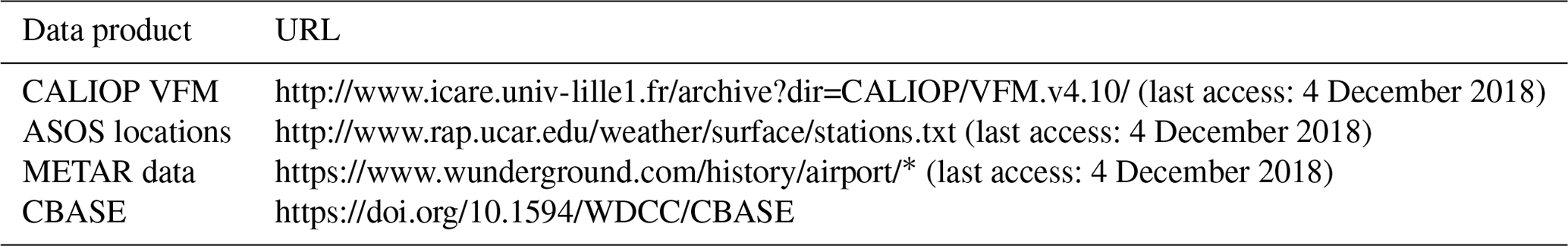
* As a first step, ASOS station identifiers within a 100 km great-circle distance of a CALIOP footprint are identified; as a second step, the ICAO identifier of the ASOS station is then used to query the Weather Underground METAR database.
Two classes of data are used in this work: cloud lidar data, from which we intend to derive a global z dataset, and ground-based observations used as reference measurements of z to train and evaluate the algorithm by which z is determined from the satellite data.
Table 1 lists the URLs for all datasets used in this paper.
2.1 CALIOP VFM
The input satellite data to our analysis are from the Cloud–Aerosol Lidar with Orthogonal Polarization (CALIOP; Winker et al., 2007) onboard the Cloud–Aerosol Lidar and Infrared Pathfinder Satellite Observation (CALIPSO) satellite that is part of the A-Train satellite constellation (Stephens et al., 2002) on a sun-synchronous low-Earth orbit with Equator crossings at approximately 13:30 local time. The cloud base product relies on the retrieved vertical feature mask (VFM; Vaughan et al., 2005). For each CALIOP lidar backscatter profile, the VFM identifies features such as clear air, cloud, aerosol, or planetary surface; this is termed the “feature type”. (When the lidar beam is completely attenuated, this is reported as a feature type.) In addition to the feature type, the VFM records the degree of confidence in the identification (“none” to “high”, termed the “feature type QA flag”), the thermodynamic phase of a layer identified as cloud as well as the degree of confidence therein (termed “ice water phase” and “ice water phase QA flag”), and the horizontal distance over which the algorithm had to average to identify a feature above noise and molecular atmospheric scattering (“horizontal averaging distance”).
In the present analysis, we use VFM version 4.10 (CALIPSO Science Team, 2016), the current standard release, for the years 2007 and 2008. The VFM files are obtained from ICARE (http://www.icare.univ-lille1.fr/, last access: 4 December 2018).
2.2 Airport ceilometers
For optimizing several parameters of the algorithm, for determining the expected cloud base uncertainty, and for evaluating the trained algorithm, reference measurements of z are required. The source of these “true” z values in this work is ground-based cloud observations at airports. Weather observations at airports are disseminated worldwide in aviation routine and special weather reports (METARs and SPECIs, collectively referred to as METARs henceforth; World Meteorological Organization, 2013). Apart from providing airport weather information for aviation, METAR data are used for assimilation into numerical weather prediction (NWP) models (e.g., Benjamin et al., 2016; Dee et al., 2011). In many locations, z reported in METARs is measured by a ceilometer over a period of time (tens of minutes) and then objectively grouped into cloud layers and their respective fractional coverages, using the temporal variation at a fixed point under an advected cloud field as a proxy for spatial variability in the cloud field (e.g., Heese et al., 2010). METAR data are widely distributed and archived; the data for the present analysis were downloaded from the Weather Underground archive (https://www.wunderground.com/history/airport/, last access: 4 December 2018).
In the US, z is mostly derived automatically by laser ceilometers that form part of the Automated Surface Observing Stations (ASOS, National Oceanic and Atmospheric Administration, Department of Defense, Federal Aviation Administration, and United States Navy, 1998) system; see, e.g., An et al. (2017) and Ikeda et al. (2017) for recent examples of ASOS application to deriving cloud climatologies or NWP model evaluation. In other parts of the world, the cloud bases may be estimated by human observers or may be omitted under certain conditions when the lowest cloud base is higher than 1524 m, complicating objective comparison to satellite z. To ensure that the ceilometer z values are of high and spatially uniform quality, we restrict ourselves to METARs from the contiguous continental US.
There are 1645 stations throughout the continental US that lie within 100 km of a CALIOP footprint. In normal operation, the time resolution of z reports is 1 h, but during rapidly changing conditions, more frequent updates may be provided; for comparison to satellite z, the ceilometer observation closest in time to the satellite overpass is used, provided that the time difference is less than 1 h. For training the algorithm, we use ceilometer observations from the year 2008. For unbiased evaluation of the algorithm performance, a statistically independent dataset is required; we use ceilometer observations from the same stations from the year 2007. Figure 1 shows the locations of these stations along with the number of satellite–ceilometer z coincidences and the closest co-location distance during the year 2007.
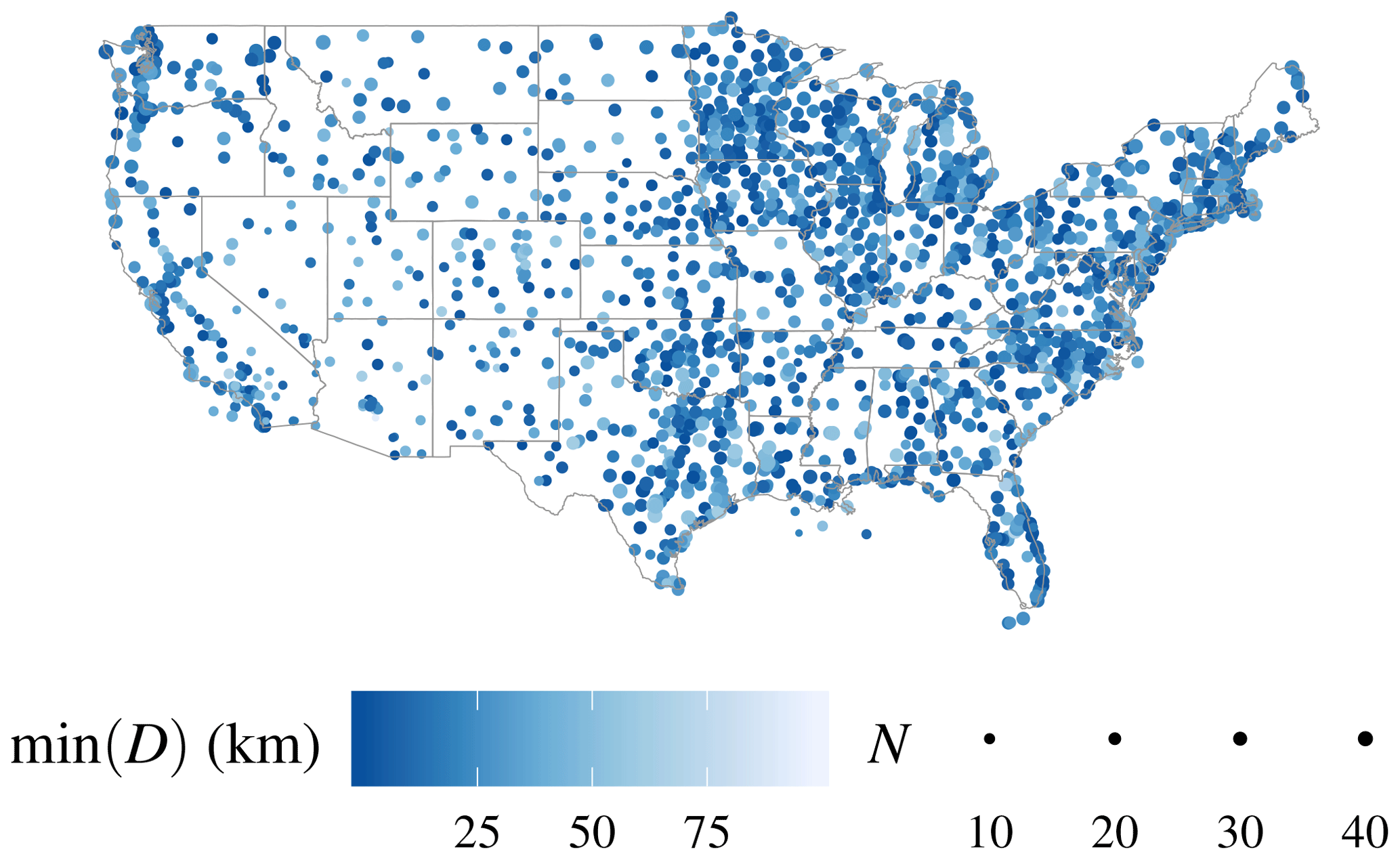
Figure 1ASOS ceilometers used for CBASE z evaluation. The size of the marker indicates the number of satellite–ceilometer z coincidences during the year 2007. Color indicates the closest co-location distance achieved in 2007.
The CBASE algorithm and evaluation proceed in four steps.
-
We determine the cloud base height from all CALIOP profiles in which the surface generates a return, indicating that the lidar is not completely attenuated by cloud. We refer to this as the column zc in the sense that it is local to the CALIOP column.
-
Using ground-based ceilometer data, we determine the quality of cloud base height depending on a number of properties of the CALIOP profile. Assuming those properties suffice to determine the quality of the zc estimate, we can then predict the quality of a cloud base as a function of those factors. The quality metric we use is the root-mean-square error (RMSE); the category RMSE determined from comparison to ceilometer zc then serves as the (sample) estimate of the predicted (population) standard deviation of the measurement error , i.e., the predicted zc uncertainty. We denote this column uncertainty as σc. In the language of machine learning, we refer to this step as training the algorithm on the ceilometer data to predict zc and σc.
-
Based on the predicted quality of each profile cloud base, we either reject the column cloud base or combine it with other cloud bases within a distance Dmax of the point of interest to arrive at an estimate of z and σ at that point. We refer to z and σ as the CBASE cloud base height and cloud base height uncertainty.
-
Using a statistically independent validation dataset, we verify that the predicted z and σ are correct.
This section is divided into four subsections, one for each algorithm step enumerated above.
3.1 Determination of CALIOP column z
Profile zc is determined from the CALIOP VFM for each profile with a surface return. The rationale is that a surface return indicates that the lidar did not attenuate within the cloud and that the lower limit of the layer identified as cloud therefore corresponds to the cloud base; Fig. 2 illustrates the idea. For these profiles, the location, zc, cloud top height, feature type between the cloud base and the surface, cloud thermodynamic phase, and associated quality assurance flags from the VFM algorithm are recorded.
3.2 Determination of CALIOP column cloud base quality
We assess the quality of the CALIOP zc using the RMSE with respect to the ceilometer-observed . The RMSE is defined as
The sum runs over all CALIOP profiles containing at least one cloud layer and a surface return that are within 100 km in horizontal distance of the ceilometer, occurring within 3600 s of a ceilometer observation, and having their lowest CALIOP cloud feature within 3 km of the surface. Ceilometer observations are only used if the observation closest in time to the CALIPSO overpass contains a cloud within 3 km of the surface. This height limit is imposed because a subset of the ceilometers has a range limit of 3810 m, and all ceilometers report ceilings above 3048 m with reduced granularity (152.4 m); the 3 km threshold is safely below these ceilometer limitations and mimics the International Satellite Cloud Climatology Project (ISCCP; Rossow and Schiffer, 1999) definition of low cloud (p>680 hPa).
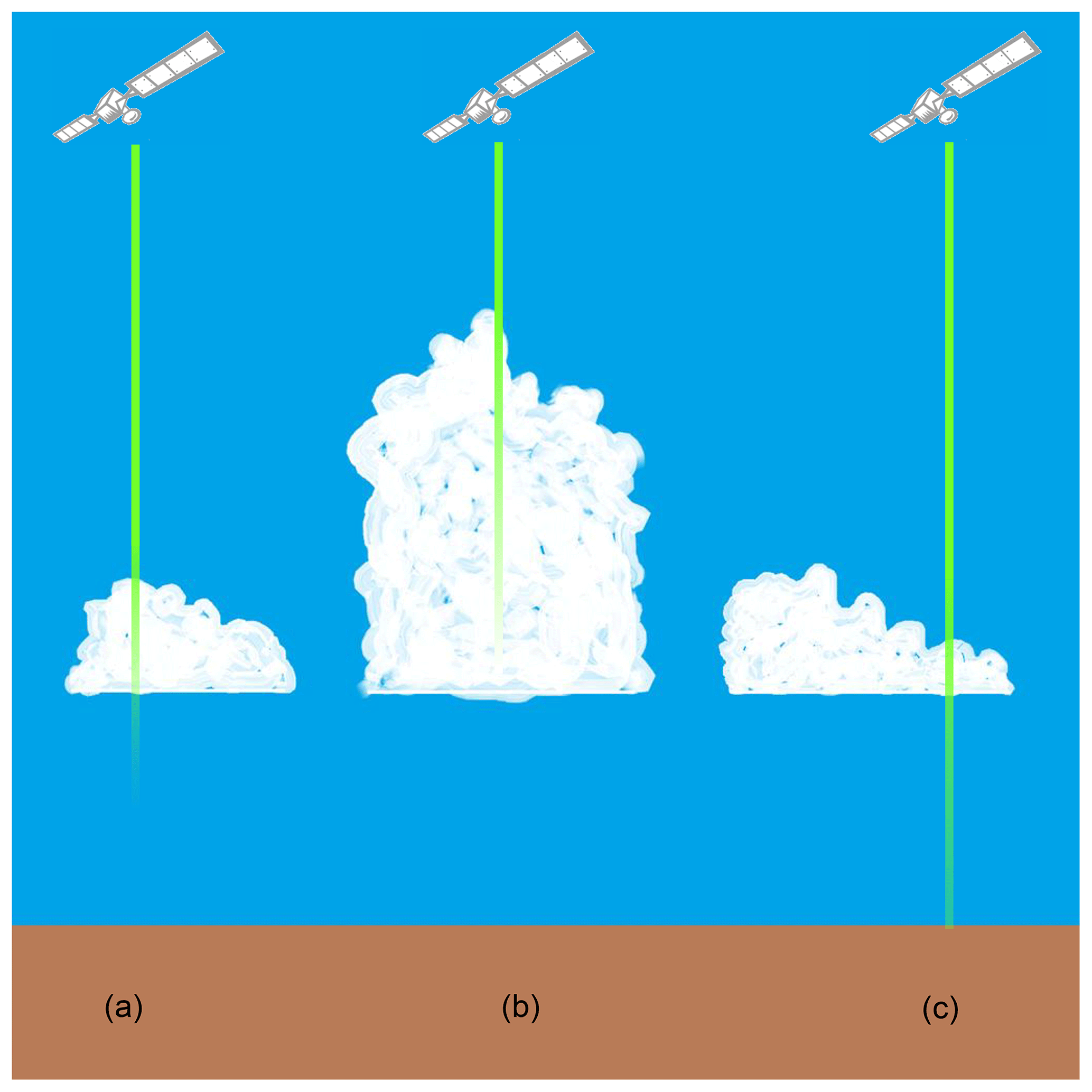
Figure 2Schematic of CALIOP cloud base determination and evaluation strategy. In optically thick clouds (a, b), the lidar attenuates significantly within the cloud, rendering the cloud base information unreliable. However, z of thin clouds (c) can be used as a proxy for thick clouds in a cloud field with homogeneous z.
The following metrics, which are useful for a qualitative assessment of the quality of the satellite cloud base, are also calculated but play no quantitative role in the algorithm:
- correlation coefficient
-
between the CALIOP cloud base and ground-based observation of the cloud base (we use the Pearson correlation coefficient, ideally unity);
- linear regression slope and intercept
-
(ideally 1 and 0, respectively);
- retrieval bias,
-
defined as
(ideally 0).
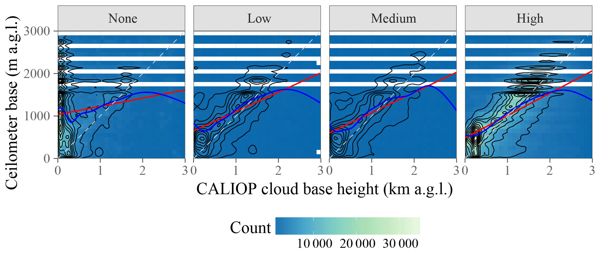
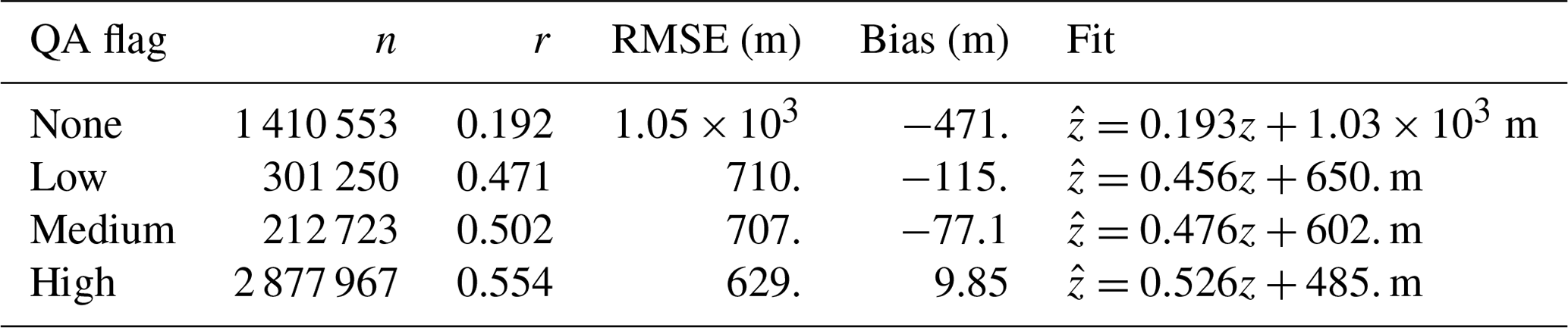
Figure 3 Scatter plots of CALIOP versus ceilometer cloud base height faceted by the CALIOP VFM QA flag; all CALIOP profiles meeting the temporal and spatial collocation requirements with a METAR enter into this plot. Color indicates the number of CALIOP profiles within each bin of ceilometer and CALIOP z; black lines are contours of the empirical joint probability density; the red line is a linear least-squares fit, with the 95 % confidence interval shaded in light red; the blue line is a generalized additive model regression (Wood, 2011), with the 95 % confidence interval shaded in light blue (due to the large dataset, the line width exceeds the confidence intervals in these plots); the dashed gray line is the one-to-one line. Statistics of the relationship between CALIOP and ceilometer base heights are provided in Table 2.
Table 2Statistics of the relationship between ceilometer and CALIOP cloud base height faceted by the CALIOP VFM QA flag. Shown are the number of CALIOP profiles n, the product-moment correlation coefficient r between CALIOP and ceilometer z, the RMSE, bias, and linear least-squares fit parameters.
CALIOP's ability to detect cloud base depends on the properties of the cloud. Therefore, we expect that the zc quality will vary among different cloud profiles. We expect that measuring the quality as a function of various properties of the CALIOP column will allow us to predict the quality of other columns with the same combination of properties. The properties that are easily accessible in a single column and have substantial effects on quality are
-
horizontal distance D from the ceilometer,
-
number of column cloud bases within horizontal distance Dmax,
-
CALIOP VFM feature quality assurance flag,
-
geometric thickness of the lowest cloud layer,
-
CALIOP thermodynamic phase determination of the lowest cloud,
-
feature type, if any, detected between the lowest cloud and the surface, and
-
horizontal averaging distance required for CALIOP cloud feature detection.
For illustrative purposes, Fig. 3 and Table 2 summarize the joint distribution of CALIOP and ceilometer zc faceted by the CALIOP VFM feature quality assurance flag.

Based on determining the retrieval quality as a function of one variable at a time (integrating over the sample distribution of the remaining variables), the following classes of CALIOP profiles are discarded:
-
CALIOP VFM quality assurance worse than “high”,
-
“invalid” or “no signal” layers between the surface and the lowest cloud layer (indicating that although the surface may generate a detectable return, the lidar is sufficiently attenuated that the cloud base, which scatters less strongly than the surface, is unreliable),
-
minimum CALIOP cloud detection horizontal averaging distance within the lowest cloud layer greater than 1 km (indicating that, although average cloud properties are known at the averaging length scale, those properties may not be representative of the particular CALIOP footprint under consideration), or
-
thermodynamic phase of the lowest layer determined to be other than liquid by the CALIOP VFM algorithm (the reason for this is that not enough such columns exist to determine the RMSE reliably in each of the categories defined below).
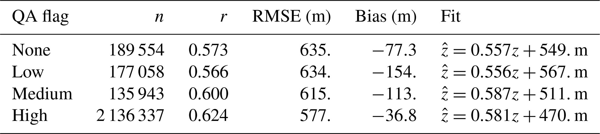
Figure 4 and Table 3 summarize the joint distribution of CALIOP profile zc and ceilometer after these selection criteria for comparison with the unfiltered joint distributions in Fig. 3.
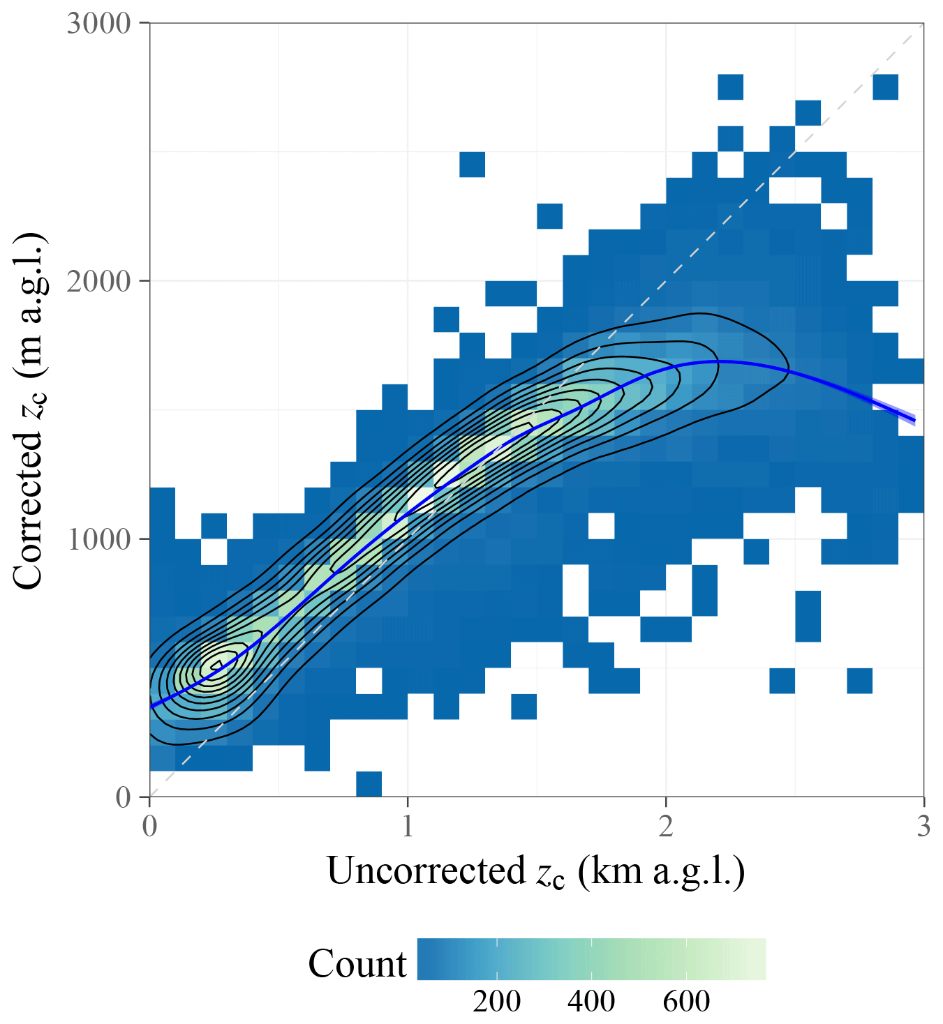
Figure 5Density estimates of the projection of the SVM correction function. The training dataset (ceilometer overpasses in 2008) is used as the ensemble for performing the projection.
The remaining variables are discretized roughly into quintiles of their distribution within the VFM dataset with the following boundaries:
-
horizontal distance D from the ceilometer, with boundaries 0, 40, 60, 75, 88, and 100 km (distance greater than 100 km is discarded);
-
number of CALIOP columns n with a cloud layer and a surface return within 100 km in horizontal distance from the ceilometer, with boundaries at 0, 175, 250, 325, and 400 (multiplicity greater than 400 is accepted); and
-
geometric thickness Δz of the lowest cloud layer, with boundaries at 0, 0.25, 0.45, 0.625, and 1 km (thickness greater than 1 km is accepted).
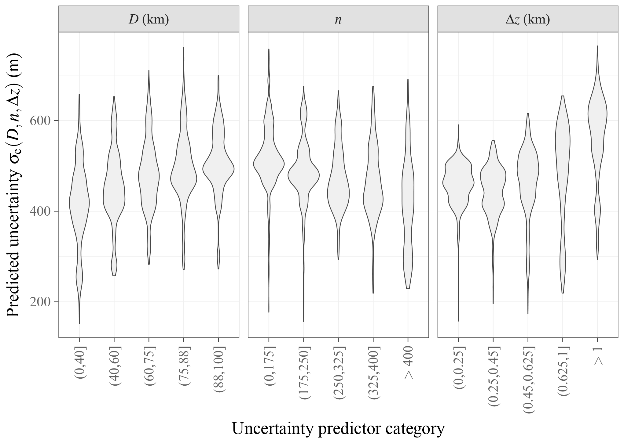
Figure 6Density estimates of the projection of onto each of the uncertainty predictor variables. The training dataset (ceilometer overpasses in 2008) is used as the ensemble for performing the projection.
We can now consider the joint distribution of CALIOP and ceilometer cloud bases for each combination of the above variables to derive the RMSE of each combination. Throughout this work, we use cloud base height above ground level (AGL); using height above mean sea level would introduce an intrinsic correlation between satellite and ceilometer cloud base height due to the varying terrain height, which would lead to an unrealistically positive assessment. To convert cloud base heights to AGL height, we subtract the surface elevation contained in the CALIOP VFM data files, which in turn comes from the CloudSat R05 surface digital elevation model.
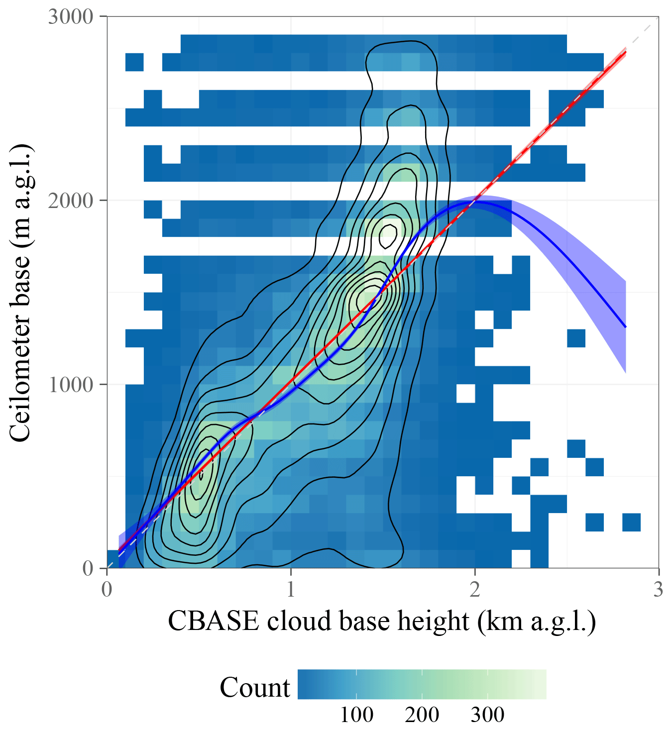
Figure 7Scatter plot of CBASE versus ceilometer z for all A-Train overpasses over the contiguous US available for 2007; for description of the plot elements, see Fig. 3. The linear fit has a slope of 0.98 and an intercept of 33.96 m.
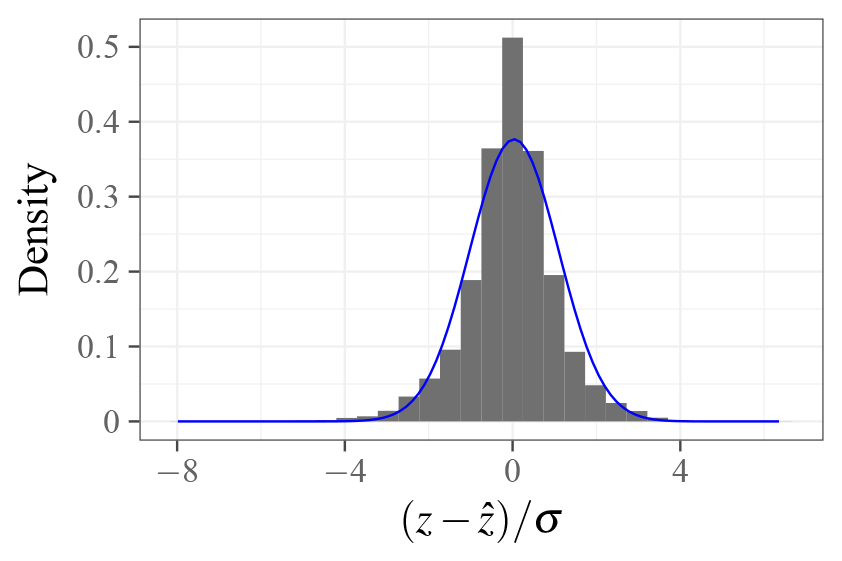
Figure 8Distribution function of cloud base error divided by predicted uncertainty; for the ideal case of unbiased z and unbiased uncertainty, the distribution would be Gaussian with zero mean and unit standard deviation. The superimposed least-squares Gaussian fit (blue line) has a mean of 0.04 and standard deviation of 1.06.
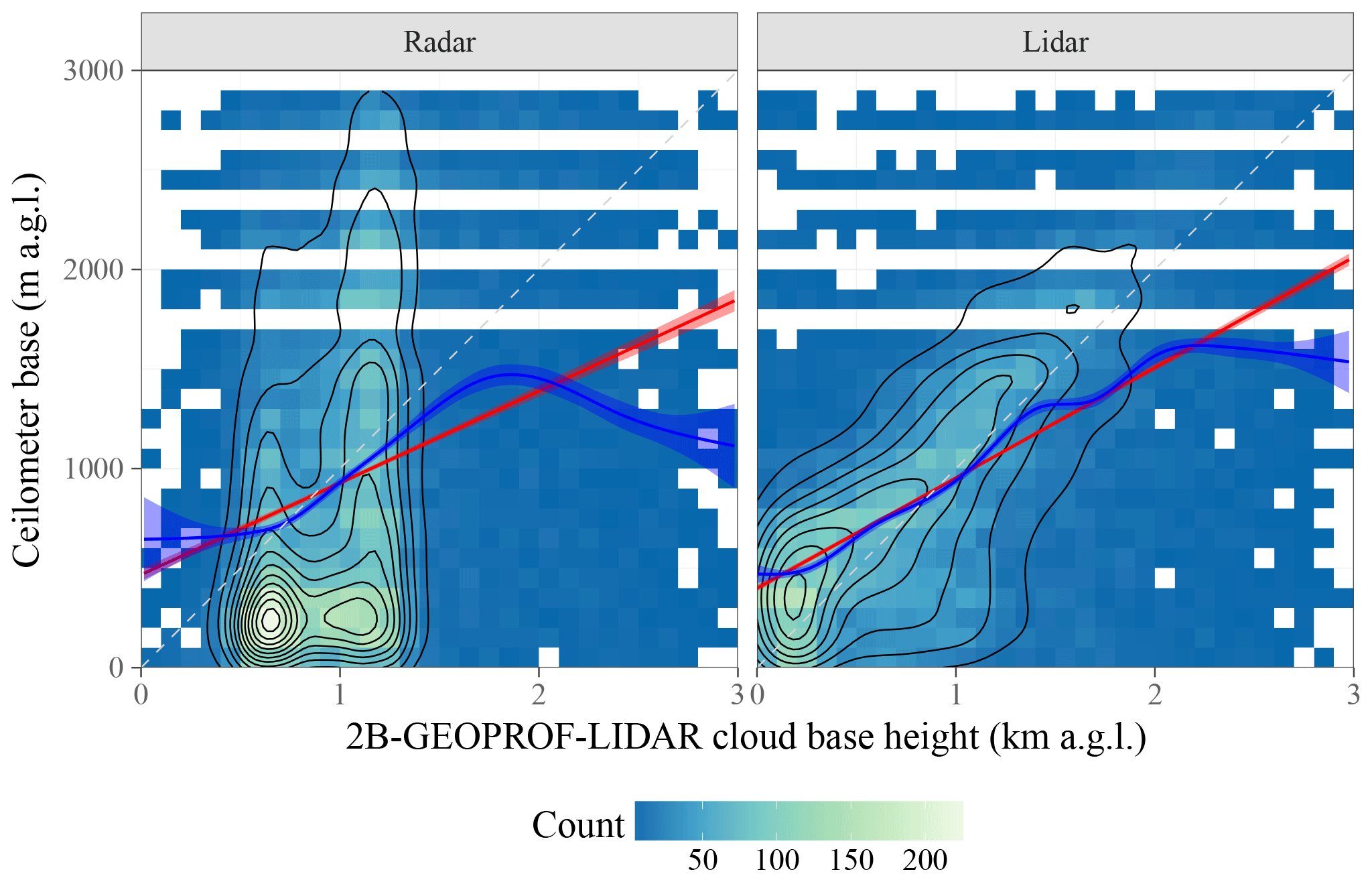
Figure 9Scatter plot of 2B-GEOPROF-LIDAR versus ceilometer z faceted by the source of the cloud base (radar only or lidar only; due to their rare occurrence, combined radar–lidar base heights are not shown). For description of the plot elements, see Fig. 3. Statistics of the relationship between 2B-GEOPROF-LIDAR and ceilometer base heights are provided in Table 5.
When calculating aggregate statistics such as the RMSE, a further consideration comes into play. zc above ground is positive-definite, which imposes a physical phase-space boundary. Due to this boundary, the satellite zc estimate is intrinsically biased high (negative excursions due to symmetric random error may be removed by the phase-space boundary, but positive excursions are not), and the bias decreases with increasing satellite zc estimate (when true zc is high, it is less likely that measurement error would lead to a negative AGL zc). Since this effect constitutes a bias rather than a random error, it cannot be eliminated by averaging over large sample sizes, but instead needs to be corrected for. Since the effect is nonlinear in zc, a nonlinear correction method is required. Our choice of nonlinear bias correction is the support vector machine (SVM; Cortes and Vapnik, 1995). The SVM is a machine-learning algorithm formulated to learn classification (Cortes and Vapnik, 1995) or regression (Vapnik, 1995) tasks from a training dataset, discarding outliers and accommodating nonlinear functions (e.g., Smola and Scholkopf, 2004). We train an ϵ-regression SVM, implemented as an R package (Meyer et al., 2018) using the LIBSVM library (Chang and Lin, 2011), separately for each D, n, and Δz category, using the 2008 ceilometer overpass training dataset. The correction function is not trivial to represent because of its dependence on zc, D, n, and Δz (which can be correlated). To reduce the dimensionality of this multivariate correction, we have used the training dataset (with its joint distribution of zc, D, n, and Δz) to calculate an ensemble of correction factors that can be expected in a realistic sample of clouds, shown in Figure 5. The full multivariate correction function, implemented in R, is available from Mülmenstädt (2018).
Following bias correction, the sample RMSE is calculated for each combination of D, n, and Δz. The sample RMSE is taken as an estimate of the statistical uncertainty σc on the CALIOP profile zc. Note that D and Δz exist for each profile, whereas n is defined for the group of suitable profiles around the point of interest. Since the predicted uncertainty is multivariate, it is also nontrivial to visualize. We again use the training dataset as an ensemble on which to perform one-dimensional projections of σc onto each of the predictor variables. These projected σc density estimates are shown in Fig. 6. The full multivariate σc prediction function, implemented in R, is available from Mülmenstädt (2018).
Table 4CBASE cloud base statistics by decile of predicted uncertainty; see Table 2 for a description of the statistics provided.

3.3 Combination of column cloud bases
CALIOP z only exists sporadically, when CALIOP happens to hit a sufficiently thin cloud. To infer the z at a point of interest that does not necessarily coincide with the location of a thin-cloud CALIOP column, we proceed as follows. We first select all CALIOP column zc measurements within a horizontal distance Dmax=100 km of the point that satisfy the additional quality cuts described in Sect. 3.2.
For each remaining column zc,i, we determine the predicted uncertainty σc,i based on the categories established in the previous section. We determine a combined z
with weights
(optimal weights for uncorrelated least squares). The sum is calculated over the n zc estimates within Dmax that satisfy all criteria listed in the previous subsection. In practice, the individual measurements of cloud base are highly correlated with fairly similar σi. The cloud base estimate by Eq. (3) with weights given by Eq. (4) remains unbiased even in the presence of correlations. However, for the combined cloud base uncertainty, the uncorrelated weights would yield a biased estimate in the presence of correlations. The expression
yields acceptable results, as would be expected for highly correlated and fairly similar σc,i.
3.4 Evaluation of CBASE z and σ
Having trained the algorithm on data from the year 2008, we evaluate it using a statistically independent dataset from the year 2007. In the evaluation dataset, the true (i.e., ceilometer-measured) is known in addition to the estimated z and the estimated cloud base uncertainty σ, determined according to the procedure described in the previous section. Figure 7 shows the joint distribution of CBASE z and ceilometer-observed .
For satellite-derived measurements of z that are unbiased with respect to the ceilometer-observed and have correctly estimated uncertainties σ, the probability density function of the quantity has zero mean and unit standard deviation. In our evaluation dataset, we find a mean of 0.04 and a standard deviation of 1.06, shown in Fig. 8; this corresponds to a z bias of 4 % and uncertainty bias of 6 %, both relative to the predicted uncertainty. Thus, we find that both the cloud base estimate and the uncertainty estimate are unbiased at better than the 10 % level.
As a further test of the reliability of the expected uncertainty, we divide the validation dataset into deciles of the expected uncertainty. Table 4 shows that the actual RMSE within each decile is within 10 % of the expected uncertainty (with the exception of the highest-uncertainty decile) and that linear regressions within each decile are close to the one-to-one line.
To check that the algorithm satisfies its design constraints (i.e., to ensure that we made no methodological error when implementing the algorithm), we have also verified that linear regression between z and has zero intercept and unit slope and that the quantity has zero mean and unit standard deviation when this validation is performed on the training dataset.
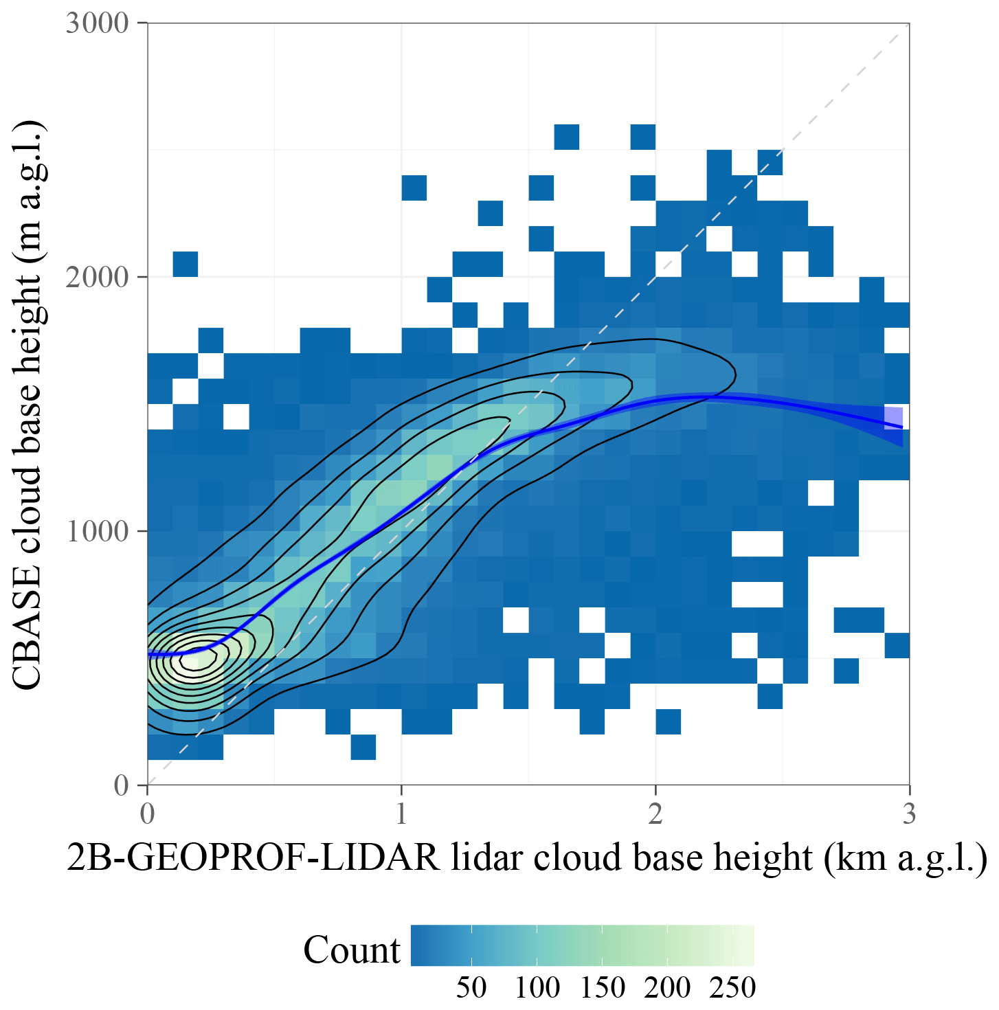
Figure 10Scatter plot of 2B-GEOPROF-LIDAR lidar-only versus CBASE z. For description of the plot elements, see Fig. 3; because both cloud base measures have comparable uncertainty, linear regression is a misleading diagnostic (Pitkanen et al., 2016) and has not been included. The mean difference between 2B-GEOPROF-LIDAR and CBASE is 0.05 km, the root-mean-square difference is 0.41 km, and the correlation coefficient is 0.79.

Figure 11Geographic distribution of mean z above ground level. Statistics are calculated within each latitude–longitude box and separately for CALIOP daytime (a) and nighttime (b) overpasses.
It is possible that z estimates outside North America could have greater biases or greater uncertainty than this evaluation leads us to believe. This would be the case if continental clouds over North America are not representative of clouds elsewhere in a way that is not accounted for by the cloud properties considered by the uncertainty estimate. Since the validation sample spans an entire year on a continental scale, we expect that most cloud morphologies are included. However, cloud types that occur predominantly over ocean, namely marine stratocumulus with horizontally extensive but vertically thin liquid-phase anvils, present a particular challenge to the method. Due to the typical z uncertainty of several hundred meters, the method is unlikely to be applied to stratocumulus cloud; nevertheless, a marine-cloud validation dataset would be desirable. For the present work, no suitable marine-cloud evaluation dataset was available; ship-based z observations were either based on human observers with coarse vertical resolution and a precision that is difficult to characterize or available only over a limited duration at limited locations, resulting in a severely statistics-limited set of coincidences with the CALIOP track.
3.5 Comparative evaluation of CBASE and 2B-GEOPROF-LIDAR
Comparison with 2B-GEOPROF-LIDAR cloud bases (version P2_R04_E02, based on the 2B-GEOPROF and CALIOP VFM products) is shown in Fig. 9. 2B-GEOPROF-LIDAR distinguishes among radar-only, lidar-only, and radar–lidar combined cloud bases; the last category is rare for warm clouds and is not shown. For radar-only clouds, the mean error is large because the radar z predominantly clusters around the top of the ground clutter region with little dependence on the actual z.
Lidar-only 2B-GEOPROF-LIDAR cloud base performs comparably to the CBASE cloud base on average; this is to be expected, as the underlying physical measurement (the CALIOP attenuated backscatter) is the same for all three products considered (2B-GEOPROF-LIDAR, CALIOP VFM, and CBASE). Figure 10 shows the relationship between CBASE z and the 2B-GEOPROF-LIDAR cloud base closest to the ceilometer for each overpass. The CBASE z for low clouds tends to be higher than the 2B-GEOPROF-LIDAR estimate because the CBASE algorithm has been designed to agree with ceilometer heights, which also tend to be higher than the 2B-GEOPROF-LIDAR estimate (see Fig. 9). Otherwise, the relationship is fairly close (linear correlation coefficient of 0.79), again as expected due to the similarity in the underlying measurement.
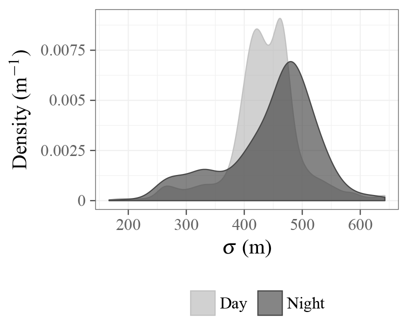
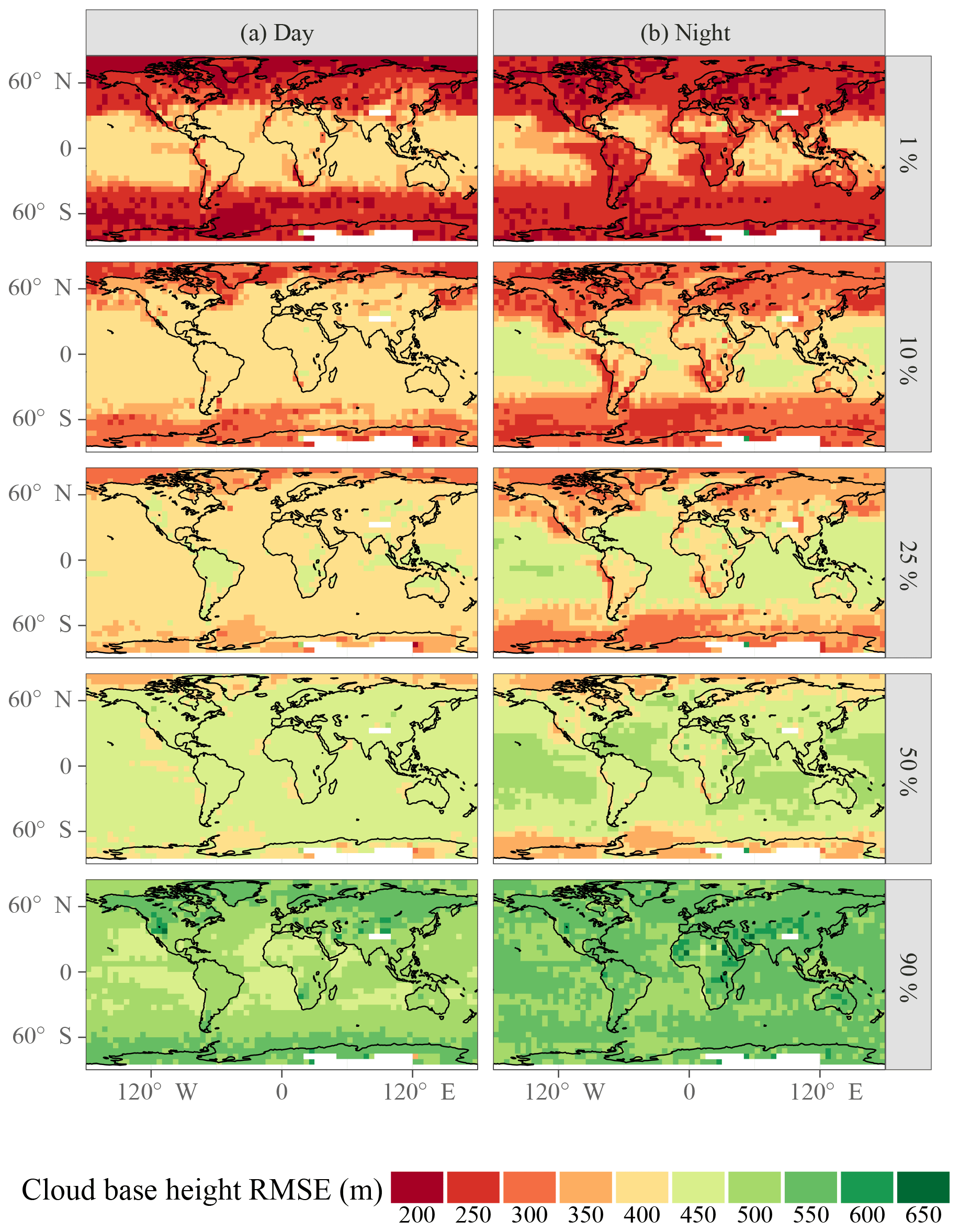
Figure 13Cloud base uncertainty quantiles. Statistics are calculated within each latitude–longitude box. Panels (a) and (b) show statistics of daytime and nighttime retrievals, respectively; daytime and nighttime are defined by the CALIOP VFM product.
Unlike 2B-GEOPROF-LIDAR and the CALIOP VFM, CBASE provides a validated point-by-point uncertainty estimate, which allows an analysis to select only low-uncertainty cases or to statistically weight z according to uncertainty, as appropriate for the application.
Table 5Statistics of the relationship between ceilometer and 2B-GEOPROF-LIDAR z; see Table 2 for a description of the statistics provided.
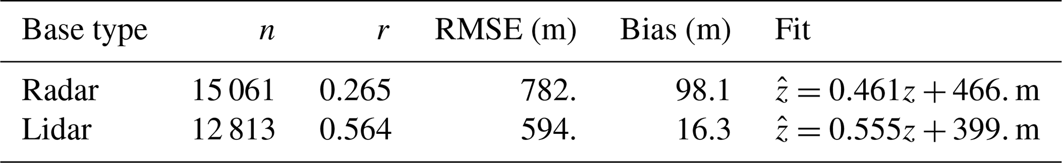
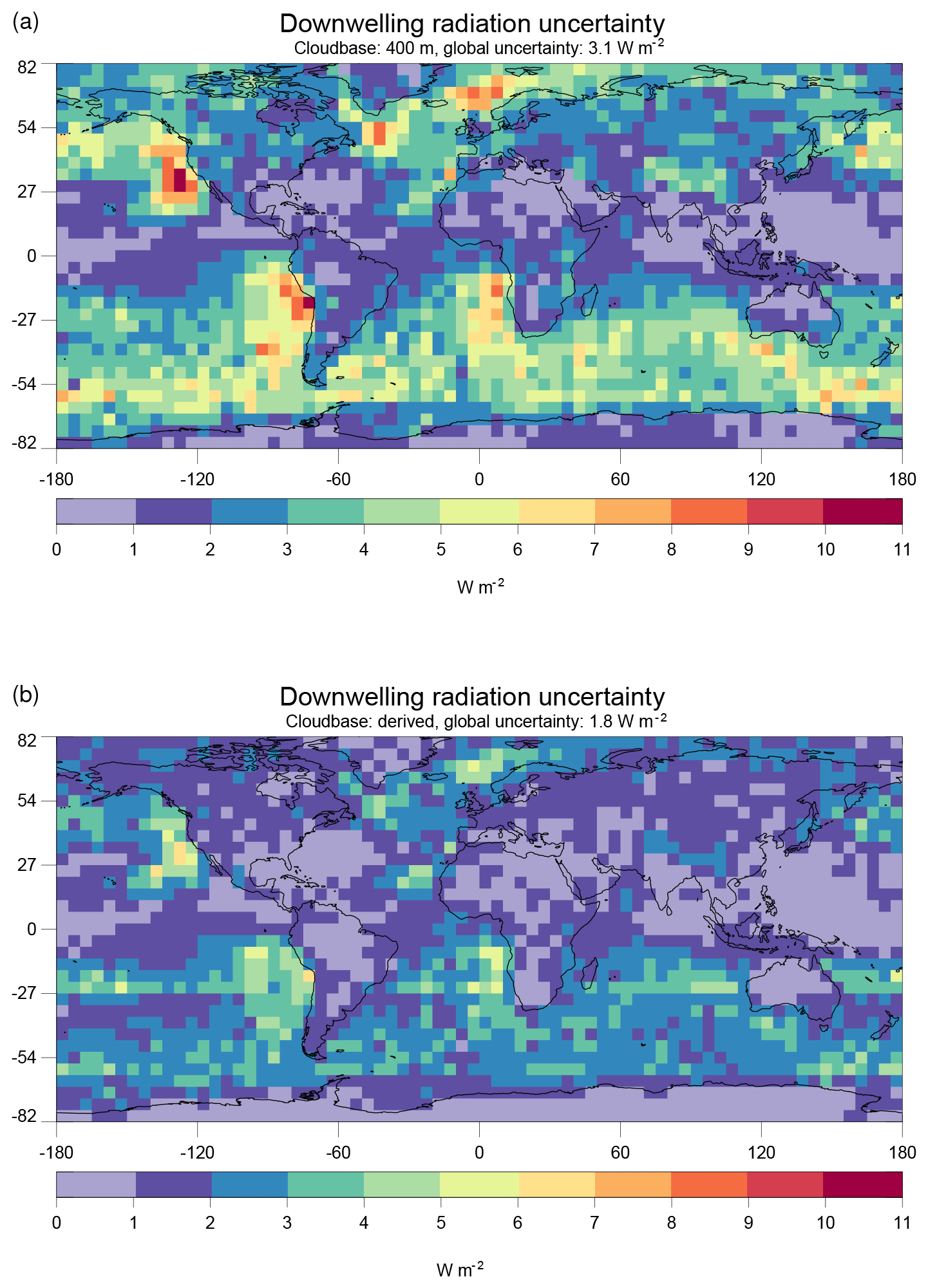
Figure 14Uncertainty on the surface downwelling longwave radiation under two assumptions of z uncertainty: (a) constant 400 m uncertainty globally and (b) uncertainty achievable by selecting a high-quality subset of CBASE z.
Geographic distributions of the mean z are shown for daytime and nighttime CALIPSO overpasses in Fig. 11. Over most of the globe, especially over land, daytime z is higher than nighttime z, consistent with the diurnal deepening of the planetary boundary layer. Figures 12 and 13 show the distribution of z uncertainties. A larger fraction of nighttime cloud bases falls into the lowest uncertainty range (200 to 350 m), while the the nighttime uncertainty distribution peaks slightly higher than the daytime uncertainty distribution and features a substantial tail above 500 m that is not present in the daytime distribution. CALIOP benefits from a higher signal-to-noise ratio during nighttime, which may lead to lower σ, but this effect would be convoluted with potential differences between daytime and nighttime clouds that can lead to different z uncertainties. Training a potential future update of the algorithm on daytime and nighttime profiles separately may reduce σ.
As an example application, we consider the surface downwelling longwave radiation , which is strongly affected by cloud base temperature. Henderson et al. (2013) derive a global sensitivity to z of 1.5 W m−2 for a z perturbation of one CloudSat height bin (240 m); as Table 5 and Fig. 9 show, the CloudSat σ specifically for the low clouds at the focus of the present work is likely greater than 240 m, which corroborates the 480 m uncertainty estimate of Kato et al. (2011). To arrive at a conservative estimate of the improvement in uncertainty that might be possible by utilizing the CBASE predicted σ, we compare two uncertainty distributions: one based on a globally constant 400 m σ (Fig. 14a) and one with the CBASE σ achievable by selecting the highest-quality percentile of the CBASE dataset (Fig. 14b). This selection provides a σ of approximately 250 m in the extratropics as well as the nighttime tropical continents and stratocumulus regions and approximately 400 m throughout the tropics during daytime, according to Fig. 13. Globally, the uncertainty is reduced from 3.1 to 1.8 W m−2, assuming that the z uncertainty contribution to the uncertainty is dominated by low clouds. Improvements are especially large in the marine stratocumulus regions and the extratropical oceans, where extensive low cloud often overlies cool air with relatively low longwave emission by water vapor. The selection reduces the available statistics by a factor of 100, but analyses based on A-Train data are usually not statistics limited.
The source code used to produce the dataset and evaluation plots is available from Mülmenstädt (2018).
The CBASE z and σ dataset (Mülmenstädt et al., 2018) spanning
the years 2007 and 2008 is freely available at Deutsches Klimarechenzentrum
(DKRZ) under the DOI https://doi.org/10.1594/WDCC/CBASE. The dataset is provided in two
spatial resolutions corresponding to different window sizes within which
CALIOP profiles are combined: Dmax=40 km and
Dmax=100 km. CBASE provides two files for each CALIOP VFM
input file: one using a 40 km window to detect the cloud field base height
and one using a 100 km window. (The input CALIOP VFM dataset is organized by
the daytime (D) and nighttime (N) half of each orbit.) The file name pattern
is CBASE - {40|100}. <
date > T < time > {D|N}.nc
(identical to the input CALIOP VFM file name with the exception of the
product name and file-type extension). Files are organized into
subdirectories by half orbit start date. In case no cloud base heights are
detected within a half-orbit, no output file is produced. Otherwise, each
CALIOP VFM input file results in a 40 km resolution and a 100 km resolution
CBASE file. The measurement quality is reported as a quantitative uncertainty
estimate for each cloud field.
We have presented the CBASE algorithm, which derives the cloud base height z from CALIOP lidar profiles. This algorithm produces z not only for thin clouds but also for clouds thick enough to attenuate the lidar (optical thickness τ≳5), based on the assumed mesoscale homogeneity of cloud base height within an air mass. In addition to the z estimate, the CBASE algorithm supplies an expected uncertainty σ on z. The CBASE dataset is available for the years 2007 and 2008 at https://doi.org/10.1594/WDCC/CBASE.
CBASE z and σ have been evaluated using ground-based airport ceilometers over the contiguous US using a data sample unbiased by the training of the algorithm. The evaluation showed that z and σ are unbiased at the level better than 10 %: the bias on z is 4 %, and the bias on the uncertainty is 6 %, both relative to the expected uncertainty.
The performance of CBASE z is similar to that of 2B-GEOPROF-LIDAR lidar-only z when validated against the same collocated ceilometer measurements, which is based on the same underlying physical measurement. However, the validated z uncertainty provided by CBASE allows for selection of only accurate cloud base heights or for statistical weighting of z according to expected uncertainty. This, in turn, makes the CBASE z useful for pressing problems in climate research that require accurate knowledge of cloud geometry, such as surface downwelling longwave radiation or cloud subadiabaticity, which will be presented in future work.
The authors declare that they have no conflict of interest.
We thank Patric Seifert and Albert Ansmann for valuable suggestions on the
algorithm; the editor and two anonymous reviewers for comments that have
improved the paper; ICARE for hosting the CALIOP VFM dataset, which was
originally obtained from the NASA Langley Research Center Atmospheric Science
Data Center; DKRZ for computing and data hosting; and the R Foundation for
Statistical Computing for providing the open-source software used for this
analysis (R Core Team, 2018). This research was funded by the European Union under ERC Starting
Grant QUAERERE, grant agreement 306284, and by the US National
Science Foundation under grant agreements AGS-1013423 and AGS-1048995.
Edited by: David Carlson
Reviewed by: two anonymous referees
An, N., Wang, K., Zhou, C., and Pinker, R. T.: Observed Variability of Cloud Frequency and Cloud-Base Height within 3600 m above the Surface over the Contiguous United States, J. Climate, 30, 3725–3742, https://doi.org/10.1175/JCLI-D-16-0559.1, 2017. a
Benjamin, S. G., Weygandt, S. S., Brown, J. M., Hu, M., Alexander, C. R., Smirnova, T. G., Olson, J. B., James, E. P., Dowell, D. C., Grell, G. A., Lin, H., Peckham, S. E., Smith, T. L., Moninger, W. R., Kenyon, J. S., and Manikin, G. S.: A North American Hourly Assimilation and Model Forecast Cycle: The Rapid Refresh, Mon. Weather Rev., 144, 1669–1694, https://doi.org/10.1175/MWR-D-15-0242.1, 2016. a
Böhm, C., Sourdeval, O., Mülmenstädt, J., Quaas, J., and Crewell, S.: Cloud base height retrieval from multi-angle satellite data, Atmos. Meas. Tech. Discuss., https://doi.org/10.5194/amt-2018-317, in review, 2018. a
CALIPSO Science Team: CALIPSO/CALIOP Level 2, Vertical Feature Mask Data, version 4.10, https://doi.org/10.5067/CALIOP/CALIPSO/LID_L2_VFM-Standard-V4-10, 2016. a
Cao, C., De Luccia, F. J., Xiong, X., Wolfe, R., and Weng, F.: Early On-Orbit Performance of the Visible Infrared Imaging Radiometer Suite Onboard the Suomi National Polar-Orbiting Partnership (S-NPP) Satellite, IEEE Trans. Geosci. Remote Sens., 52, 1142–1156, https://doi.org/10.1109/TGRS.2013.2247768, 2014. a
Chang, C.-C. and Lin, C.-J.: LIBSVM: A library for support vector machines, ACM Trans. Intellig. Syst. Technol., 2, 27:1–27:27, available at: http://www.csie.ntu.edu.tw/~cjlin/libsvm (last access: 4 December 2018), 2011. a
Cortes, C. and Vapnik, V.: Support-Vector Networks, Machine Learn., 20, 273–297, https://doi.org/10.1023/A:1022627411411, 1995. a, b
Dee, D. P., Uppala, S. M., Simmons, A. J., Berrisford, P., Poli, P., Kobayashi, S., Andrae, U., Balmaseda, M. A., Balsamo, G., Bauer, P., Bechtold, P., Beljaars, A. C. M., van de Berg, L., Bidlot, J., Bormann, N., Delsol, C., Dragani, R., Fuentes, M., Geer, A. J., Haimberger, L., Healy, S. B., Hersbach, H., Holm, E. V., Isaksen, L., Kallberg, P., Koehler, M., Matricardi, M., McNally, A. P., Monge-Sanz, B. M., Morcrette, J.-J., Park, B.-K., Peubey, C., de Rosnay, P., Tavolato, C., Thepaut, J.-N., and Vitart, F.: The ERA-Interim reanalysis: configuration and performance of the data assimilation system, Q. J. Roy. Meteorol. Soc., 137, 553–597, https://doi.org/10.1002/qj.828, 2011. a
Diner, D. J., Beckert, J. C., Reilly, T. H., Bruegge, C. J., Conel, J. E., Kahn, R. A., Martonchik, J. V., Ackerman, T. P., Davies, R., Gerstl, S. A. W., Gordon, H. R., Muller, J. P., Myneni, R. B., Sellers, P. J., Pinty, B., and Verstraete, M. M.: Multi-angle Imaging SpectroRadiometer (MISR) – Instrument description and experiment overview, IEEE Trans. Geosci. Remote Sens., 36, 1072–1087, https://doi.org/10.1109/36.700992, 1998. a
Fitch, K. E., Hutchison, K. D., Bartlett, K. S., Wacker, R. S., and Gross, K. C.: Assessing VIIRS cloud base height products with data collected at the Department of Energy Atmospheric Radiation Measurement sites, Int. J. Remote Sens., 37, 2604–2620, https://doi.org/10.1080/01431161.2016.1182665, 2016. a
Goren, T., Rosenfeld, D., Sourdeval, O., and Quaas, J.: Satellite Observations of Precipitating Marine Stratocumulus Show Greater Cloud Fraction for Decoupled Clouds in Comparison to Coupled Clouds, Geophys. Res. Lett., 45, 5126–5134, https://doi.org/10.1029/2018GL078122, 2018. a
Heese, B., Flentje, H., Althausen, D., Ansmann, A., and Frey, S.: Ceilometer lidar comparison: backscatter coefficient retrieval and signal-to-noise ratio determination, Atmos. Meas. Tech., 3, 1763–1770, https://doi.org/10.5194/amt-3-1763-2010, 2010. a
Henderson, D. S., L'Ecuyer, T., Stephens, G., Partain, P., and Sekiguchi, M.: A Multisensor Perspective on the Radiative Impacts of Clouds and Aerosols, J. Appl. Meteorol. Climatol., 52, 853–871, https://doi.org/10.1175/JAMC-D-12-025.1, 2013. a
Ikeda, K., Steiner, M., and Thompson, G.: Examination of Mixed-Phase Precipitation Forecasts from the High-Resolution Rapid Refresh Model Using Surface Observations and Sounding Data, Weather Forecast., 32, 949–967, https://doi.org/10.1175/WAF-D-16-0171.1, 2017. a
Kato, S., Rose, F. G., Sun-Mack, S., Miller, W. F., Chen, Y., Rutan, D. A., Stephens, G. L., Loeb, N. G., Minnis, P., Wielicki, B. A., Winker, D. M., Charlock, T. P., Stackhouse, P. W. J., Xu, K.-M., and Collins, W. D.: Improvements of top-of-atmosphere and surface irradiance computations with CALIPSO-, CloudSat-, and MODIS-derived cloud and aerosol properties, J. Geophys. Res.-Atmos., 116, D19209, https://doi.org/10.1029/2011JD016050, 2011. a
Kokhanovsky, A. A. and Rozanov, V. V.: Cloud bottom altitude determination from a satellite, IEEE Geosci. Remote Sens. Lett., 2, 280–283, https://doi.org/10.1109/LGRS.2005.846837, 2005. a
Lelli, L. and Vountas, M.: Chapter 5 – Aerosol and Cloud Bottom Altitude Covariations From Multisensor Spaceborne Measurements, in: Remote Sensing of Aerosols, Clouds, and Precipitation, edited by: Islam, T., Hu, Y., Kokhanovsky, A., and Wang, J., 109 – 127, Elsevier, https://doi.org/10.1016/B978-0-12-810437-8.00005-0, 2018. a
Mace, G. G. and Zhang, Q.: The CloudSat radar-lidar geometrical profile product (RL-GeoProf): Updates, improvements, and selected results, J. Geophys. Res.-Atmos., 119, 9441–9462, https://doi.org/10.1002/2013JD021374, 2014. a, b
Marchand, R., Mace, G. G., Ackerman, T., and Stephens, G.: Hydrometeor detection using Cloudsat – An earth-orbiting 94-GHz cloud radar, J. Atmos. Ocean. Technol., 25, 519–533, https://doi.org/10.1175/2007JTECHA1006.1, 2008. a, b
Meerkoetter, R. and Zinner, T.: Satellite remote sensing of cloud base height for convective cloud fields: A case study, Geophys. Res. Lett., 34, L17805, https://doi.org/10.1029/2007GL030347, 2007. a
Meyer, D., Dimitriadou, E., Hornik, K., Weingessel, A., and Leisch, F.: e1071: Misc Functions of the Department of Statistics, Probability Theory Group (Formerly: E1071), TU Wien, available at: https://CRAN.R-project.org/package=e1071 (last access: 4 December 2018), R package version 1.7-0, 2018. a
Mülmenstädt, J.: jmuelmen/cbase-essd: Version used for ESSD description paper, Zenodo, https://doi.org/10.5281/zenodo.1560603, 2018. a, b, c
Mülmenstädt, J., Sourdeval, O., Henderson, D. S., L'Ecuyer, T. S., Unglaub, C., Jungandreas, L., Böhm, C., Russell, L. M., and Quaas, J.: Using CALIOP to estimate cloud-field base height and its uncertainty: the Cloud Base Altitude Spatial Extrapolator (CBASE) algorithm and dataset, version 1.0, https://doi.org/10.1594/WDCC/CBASE, 2018. a
National Oceanic and Atmospheric Administration, Department of Defense, Federal Aviation Administration, and United States Navy: Automated Surface Observing System User's Guide, available at: http://www.nws.noaa.gov/asos/pdfs/aum-toc.pdf (last access: 4 December 2018), 1998. a
Naud, C. M., Muller, J. P., Clothiaux, E. E., Baum, B. A., and Menzel, W. P.: Intercomparison of multiple years of MODIS, MISR and radar cloud-top heights, Ann. Geophys., 23, 2415–2424, 2005. a
Naud, C. M., Baum, B. A., Pavolonis, M., Heidinger, A., Frey, R., and Zhang, H.: Comparison of MISR and MODIS cloud-top heights in the presence of cloud overlap, Remote Sens. Environ., 107, 200–210, https://doi.org/10.1016/j.rse.2006.09.030, 2007. a
Pitkanen, M. R. A., Mikkonen, S., Lehtinen, K. E. J., Lipponen, A., and Arola, A.: Artificial bias typically neglected in comparisons of uncertain atmospheric data, Geophys. Res. Lett., 43, 10003–10011, https://doi.org/10.1002/2016GL070852, 2016. a
Platnick, S., Meyer, K. G., King, M. D., Wind, G., Amarasinghe, N., Marchant, B., Arnold, G. T., Zhang, Z., Hubanks, P. A., Holz, R. E., Yang, P., Ridgway, W. L., and Riedi, J.: The MODIS Cloud Optical and Microphysical Products: Collection 6 Updates and Examples From Terra and Aqua, IEEE Trans. Geosci. Remote Sens., 55, 502–525, https://doi.org/10.1109/TGRS.2016.2610522, 2017. a
R Core Team: R: A Language and Environment for Statistical Computing, R Foundation for Statistical Computing, Vienna, Austria, available at: https://www.R-project.org/, last access: 4 December 2018. a
Rossow, W. B. and Schiffer, R. A.: Advances in understanding clouds from ISCCP, B. Am. Meteorol. Soc., 80, 2261–2287, https://doi.org/10.1175/1520-0477(1999)080<2261:AIUCFI>2.0.CO;2, 1999. a
Sassen, K. and Wang, Z.: Classifying clouds around the globe with the CloudSat radar: 1-year of results, Geophys. Res. Lett., 35, L04805, https://doi.org/10.1029/2007GL032591, 2008. a
Smola, A. J. and Scholkopf, B.: A tutorial on support vector regression, Stat. Comput., 14, 199–222, https://doi.org/10.1023/B:STCO.0000035301.49549.88, 2004. a
Stephens, G. L., Vane, D. G., Boain, R. J., Mace, G. G., Sassen, K., Wang, Z. E., Illingworth, A. J., O'Connor, E. J., Rossow, W. B., Durden, S. L., Miller, S. D., Austin, R. T., Benedetti, A., and Mitrescu, C.: The CloudSat mission and the A-Train – A new dimension of space-based observations of clouds and precipitation, B. Am. Meteorol. Soc., 83, 1771–1790, https://doi.org/10.1175/BAMS-83-12-1771, 2002. a
Tanelli, S., Durden, S. L., Im, E., Pak, K. S., Reinke, D. G., Partain, P., Haynes, J. M., and Marchand, R. T.: CloudSat's Cloud Profiling Radar After Two Years in Orbit: Performance, Calibration, and Processing, IEEE Trans. Geosci. Remote Sens., 46, 3560–3573, https://doi.org/10.1109/TGRS.2008.2002030, 2008. a
Vapnik, V. N.: The Nature of Statistical Learning Theory, Springer, New York, NY, https://doi.org/10.1007/978-1-4757-3264-1, 1995. a
Vaughan, M. A., Winker, D. M., and Powell, K. A.: CALIOP Algorithm Theoretical Basis Document Part 2: Feature Detection and Layer Properties Algorithms, available at: https://www-calipso.larc.nasa.gov/resources/pdfs/PC-SCI-202_Part2_rev1x01.pdf (last access: 4 December 2018), 2005. a
Winker, D. M., Hunt, W. H., and McGill, M. J.: Initial performance assessment of CALIOP, Geophys. Res. Lett., 34, L19803, https://doi.org/10.1029/2007GL030135, 2007. a
Wood, S. N.: Fast stable restricted maximum likelihood and marginal likelihood estimation of semiparametric generalized linear models, J. Roy. Stat. Soc. (B), 73, 3–36, 2011. a
World Meteorological Organization: Techincal Regulations Volume II: Meteorological service for international air navigation, available at: https://library.wmo.int/pmb_ged/wmo_49-v2_2013_en.pdf (last access: 4 December 2018), 2013. a
Zhu, Y., Rosenfeld, D., Yu, X., Liu, G., Dai, J., and Xu, X.: Satellite retrieval of convective cloud base temperature based on the NPP/VIIRS Imager, Geophys. Res. Lett., 41, 1308–1313, https://doi.org/10.1002/2013GL058970, 2014. a