the Creative Commons Attribution 4.0 License.
the Creative Commons Attribution 4.0 License.
 | 14 Mar 2018
Hourly mass and snow energy balance measurements from Mammoth Mountain, CA USA, 2011–2017
Robert E. Davis
Jeff Dozier
The mass and energy balance of the snowpack govern its evolution. Direct measurement of these fluxes is essential for modeling the snowpack, yet there are few sites where all the relevant measurements are taken. Mammoth Mountain, CA USA, is home to the Cold Regions Research and Engineering Laboratory and University of California – Santa Barbara Energy Site (CUES), one of five energy balance monitoring sites in the western US. There is a ski patrol study site on Mammoth Mountain, called the Sesame Street Snow Study Plot, with automated snow and meteorological instruments where new snow is hand-weighed to measure its water content. There is also a site at Mammoth Pass with automated precipitation instruments. For this dataset, we present a clean and continuous hourly record of selected measurements from the three sites covering the 2011–2017 water years. Then, we model the snow mass balance at CUES and compare model runs to snow pillow measurements. The 2011–2017 period was marked by exceptional variability in precipitation, even for an area that has high year-to-year variability. The driest year on record, and one of the wettest years, occurred during this time period, making it ideal for studying climatic extremes. This dataset complements a previously published dataset from CUES containing a smaller subset of daily measurements. In addition to the hand-weighed SWE, novel measurements include hourly broadband snow albedo corrected for terrain and other measurement biases. This dataset is available with a digital object identifier: https://doi.org/10.21424/R4159Q.
- Article
(4347 KB) -
Supplement
(2181 KB) - BibTeX
- EndNote


The mass and energy balance of the snowpack govern its evolution. Direct measurement of the variables that comprise these balances is critical to our understanding of the snowpack. Monitoring of the snowpack energy and mass balance has broad utility as the timing and rate of snowmelt affect over 60 million people in the western US (Bales et al., 2006) and a billion people worldwide (Barnett et al., 2005). Yet, direct measurement of all necessary variables is rare, especially at high-altitude sites. Additionally, there are some variables, such as the broadband snow albedo, which require substantial and nontrivial adjustments that require detailed information on measurement location. This partly explains why high-quality datasets of snow albedo, a driver for snowmelt for many parts of the world (e.g., Marks and Dozier, 1992; Painter et al., 2018; van den Broeke et al., 2011), are rare.
In the western US, there are five such sites where the full energy balance is monitored (Bales et al., 2006). One of these sites is the Cold Regions Research and Engineering Laboratory and University of California – Santa Barbara Energy Site (CUES). CUES has many unique features and, over the decades, has been home to numerous snow hydrology and snow avalanche studies. Bair et al. (2015) describe the history of CUES, summarize current measurements, and provide three case studies using these measurements. We provide here an expansive dataset, with hourly measurements of all the variables required to model the snow mass and energy balance.
CUES (37.643∘ N, 119.029∘ W) is located at 2940 m, midway up Mammoth Mountain, CA USA (Fig. 1). The Sesame Snow Study Plot (37.650∘ N, 119.042∘ W, elevation 2743 m), hereafter called Sesame, is located just above the Main Lodge at Mammoth Mountain (Fig. 1). Mammoth Pass (37.612∘ N, 119.032∘ W, elevation 2835 m), hereafter called MHP, is located near McCloud Lake, just to the south of Mammoth Mountain (Fig. 1). Mammoth Mountain is a silica dome cluster (Hildreth, 2004) in the central Sierra Nevada. It is an active volcano with eruptions as recent as 300 to 700 years ago, based on evidence from radiocarbon-dated samples of charred wood (Bailey, 1989). There are several active fumaroles on Mammoth Mountain, and its surface is covered by volcanic deposits. As it relates to snow hydrology and albedo degradation, large portions of Mammoth Mountain are coved by tephra or pumice. In fact, prior to being named Mammoth Mountain, it was rumoured to have been called Pumice Mountain by local inhabitants. Strong winds often blow pumice onto the snow surface and this significantly degrades its albedo (Sterle et al., 2013).
One of the largest ski areas in North America, Mammoth Mountain currently has 28 ski lifts, including a gondola that operates nearly year-round, making CUES highly accessible relative to other high-altitude scientific research sites, including the Senator Beck (Landry et al., 2014) and Reynolds Creek (Slaughter et al., 2001) sites. With an average peak SWE of 128 cm, CUES also has a much deeper snowpack than the five long-term energy balance sites in the western US, although its snow climate is not strictly maritime due to infrequent winter rain (Bair, 2013).
The CUES site itself is located on a small plateau, with a year-round roped-off perimeter to prevent disturbance. Vegetation consists of loosely spaced trees, mostly Whitebark and Lodgepole Pine, with some shrubs in the understory that are usually buried after the first significant snowfall. The loosely spaced trees and its topography give CUES exposure to most of the sky, but also expose the site to strong winds that make accurate measurement of precipitation with typical weighing gauges impossible. Instead, snow depth sensors and snow pillows are used. For precipitation, we use data from Sesame (Bair, 2013) and MHP. Unlike CUES, Sesame is located in a small opening in a Whitebark Pine forest, also with a roped-off perimeter when there is snow cover. The understory here also consists of small shrubs. Ground cover is also predominately tephra. MHP is also located in a Whitebark Pine forest with similar understory and ground cover to Sesame.

Figure 1Satellite imagery of Mammoth Mountain on 4 February 2017 showing Sesame, CUES, and MHP. The satellite image is from DigitalGlobe Worldview-3. ® 2018 DigitalGlobe NextView License.
2.1 Sesame
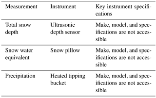
The automated hourly measurements in this dataset from Sesame are air temperature; relative humidity; snow depth; and SWE. Sources (e.g., measured or interpolated) are given for each automated measurement. The manual measurements include new (24 h) snow, new SWE, rainfall observations, and notes.
Table 1List of measurements and instruments used in this dataset at the Sesame Snow Study Plot. Instrument specifications are from the manufacturer unless noted and cited.
Hand-weighed snowfall measurements every 24 h at Sesame (Fig. 2) are made on a white wooden board that is cleared daily each time enough snow falls to be accurately weighed (a few centimeters). At least two cores are made and the average is taken. We provide all the manual Sesame measurements (Table 1) for days with precipitation, based on the morning daily weather observations, posted as the “Storm Summaries” on http://patrol.mammothmountain.com. Rounding to the nearest hour, these measurements are almost always recorded at 07:00.
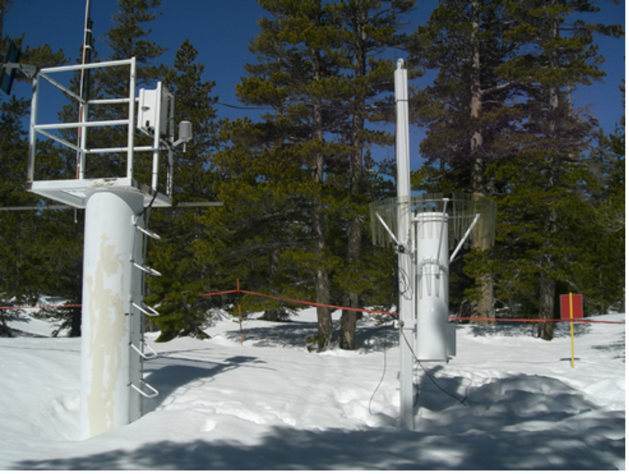
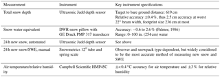
Figure 2Sesame Snow Study Plot in April 2006. On the left is the tower where total snow depth is measured using a boom. On the right is a weighing gauge, manually raised and lowered about 1 m above the snow surface.
Sesame also has two automated precipitation gauges, a Met One 385 Rain Gauge tipping bucket and a Sutron Total Precipitation weighing gauge, both with 1 min readings. The measurements from these gauges have large gaps from times when they were not working, making them unsuitable for a continuous hourly dataset. Specifically, the Met One 385 had repeated heating problems that required replacement of the heating element and the Sutron showed noise and undercatch problems. Sesame has two ultrasonic Judd snow depth sensors also, one for the 24 h board and one to measure the total snow depth. We provide the total depth here, as the automated 24 h board snow depth measurements are more useful for operational purposes and can be difficult to interpret, for instance when the board is being cleared. A snow pillow was installed by the California Department of Water Resources (DWR) and the first author in October 2013. It has had continuous measurements since then, except for a period starting sometime around February 2017 when the pressure transducer failed, presumably because of the exceptional weight of the snowpack. The transducer was replaced in July 2017. Likewise, a Lufft WS600-UMB Smart Weather Sensor was installed at Sesame in January 2012. This sensor is equipped with a Doppler radar and uses a mass fallspeed relationship to estimate precipitation rates. For liquid precipitation this method works quite well (Löffler-Mang et al., 1999), but for solid precipitation, this method requires assumptions about the snowflake mass and other properties, giving an inaccurate snowfall rate (Matrosov, 2007). We have noted inaccurate results when comparing the WS600 estimates to the hand-weighed estimates at Sesame. Additionally, the WS600 shows many false positives for precipitation when no precipitation occurs. The WS600 is useful at Sesame because it contains a sonic anemometer that measures wind speed, and this wind speed measurement can be used to correct for undercatch in the precipitation gauges (Goodison et al., 1998). Comparisons of hand-weighed and automated measurements at Sesame show an undercatch of 9 % on average.
Since Sesame is an operational ski area site, precipitation measurements during the summer are generally not taken. We suggest this is not a significant problem given our focus on snow mass and energy balance measurements. Also, summer rainfall in the Sierra Nevada is a small fraction of total precipitation. In the Sierra Nevada, October through May precipitation accounts for about 95 % of annual precipitation (NOAA National Climatic Data Center, 2017). Nonetheless, we emphasize to the reader that reliable precipitation estimates from Sesame only comprise periods starting with the season's first snowfall, usually in October, prior to the opening of the ski area, until the ski area closes, usually between 31 May and 4 July.
2.2 MHP
The automated hourly measurements in this dataset from MHP are snow depth; SWE; and precipitation. Sources (e.g., measured or interpolated) are given for each automated measurement.
Mammoth Pass (Fig. 3) is one of the older snow course locations in the area. The Los Angeles Department of Water and Power started weighing snow cores here in 1926.
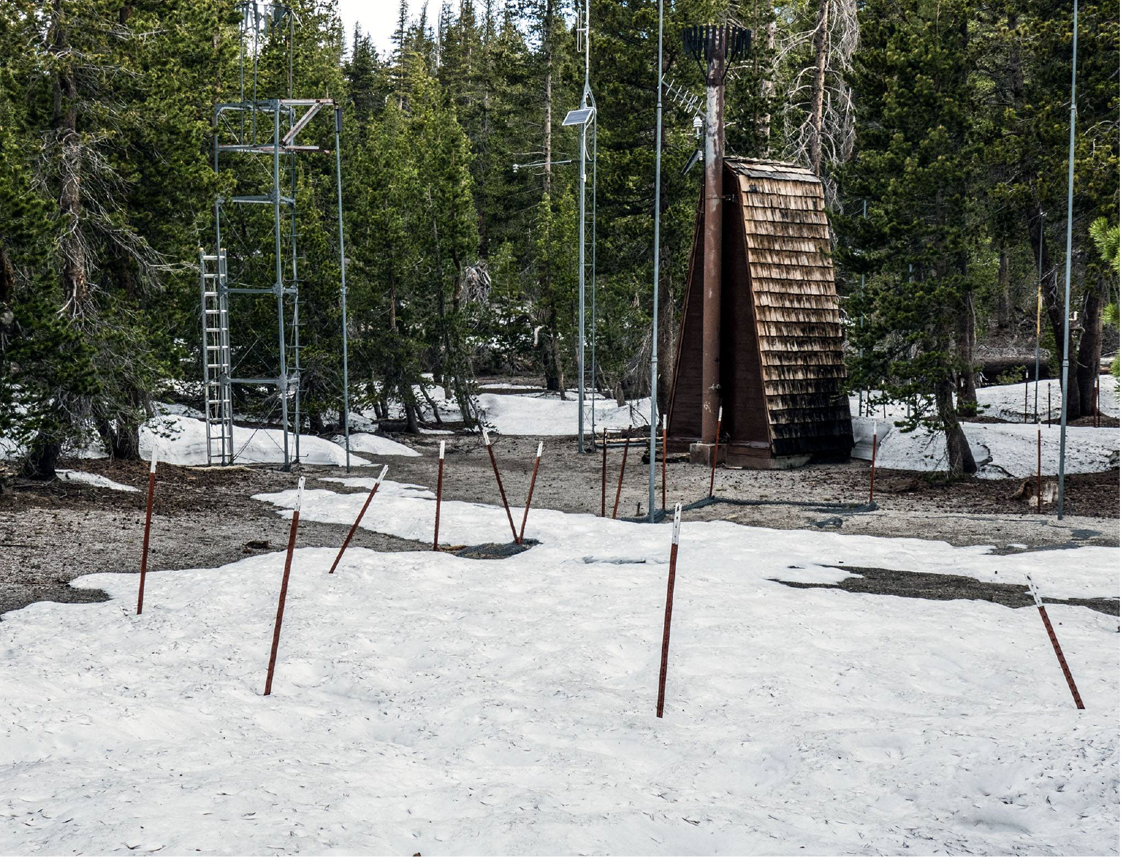
Figure 3MHP on 10 June 2016. The snow pillow is marked by the brown metal stakes. The tipping bucket is also painted brown and can be identified by its black Alter shield. The ultrasonic depth sensor is on the boom below the solar panel. Photo courtesy of Rick Kattelmann.
Automated daily measurements are available here back until 1989, with hourly measurements back to 1998. Currently, there is a heated tipping bucket precipitation gauge, an air temperature sensor, an ultrasonic snow depth sensor, and a snow pillow. Data are collected hourly via a satellite modem. Manufacturer, model, and other instrument metadata were not available to us. Mammoth Pass measurements are available in the California Data Exchange Center (California Department of Water Resources, 2018) using station code MHP.
2.3 CUES
The automated hourly measurements in this dataset from CUES are uplooking broadband radiation; uplooking direct solar radiation; uplooking diffuse solar radiation; direct broadband snow albedo; uplooking longwave radiation; wind speed; wind direction; ground temperature; air temperature; relative humidity; air pressure; snow depth; and SWE. Sources (e.g., measured or interpolated) are given for each automated measurement.
As with Sesame, mass balance measurements are focused on the snow accumulation and ablation season at CUES (Fig. 4). The site operates year-round, but as discussed earlier, there are no reliable precipitation gauge measurements, as the site is too windy for reasonable catch efficiencies. As with Sesame, a Lufft WS600-UMB was installed at CUES in October 2011, but given the inaccuracies and our experience with this sensor described in Sect. 2.1 and since its measurements do not cover the entire study period, we have not included its measurements in this dataset.
Figure 4A nearly buried CUES platform in February 2017. The RM Young 5103 is the white anemometer with a propeller. The ultrasonic Judd depth sensor is mounted above a snow pillow on the boom attached to the white H-beam on the right side of the image. The snow depth has reached the CUES platform, 6 m above the ground, several times since 1987, but never completely buried it.
A snow pillow was installed by the DWR in September 2012 and CUES has hosted experimental fluidless and other snow pillows in the past. Snowfall is measured most consistently at CUES using ultrasonic snow depth sensors (Table 2). Currently, there are three sensors at the site. For this study, an ultrasonic Judd depth sensor located directly above the DWR snow pillow was used (Table 2).
To aggregate sub-hourly measurements to 1 h, we employed forward-looking averages, meaning that the average for say 12:00 contains the average of all measurements from 12:00 to 12:59. This is important to note, as data loggers often employ a reverse-looking average; e.g., for this case the 12:00 average would contain all measurements from 11:00 to 11:59. The two methods can be easily converted between by adding or subtracting 1 h from the “DateTime” field. All of the hourly measurements were aggregated this way in the database, but the MHP measurements were only available as reverse-looking averages; therefore, they were shifted by 1 h forward to match.
3.1 Energy balance measurements
The full suite of energy balance measurements come from CUES. Some of these measurements, such as the incoming radiation, are available going back to 1992 at http://www.snow.ucsb.edu.
3.1.1 Air temperature, relative humidity, ground temperature, and air pressure measurements
Air temperature and relative humidity are measured at CUES and Sesame simultaneously using radiation-shielded Campbell HMP 45C sensors (Table 1 and Table 2). Ground temperature is measured at CUES using a buried thermistor string. The highest depth, labeled “0 cm”, was used, which corresponds to the soil layer just beneath the surface. Atmospheric pressure is measured at CUES using a Met One 092 barometer pressure sensor.
3.1.2 Wind speed and direction measurements
Wind speed and direction are measured at CUES using three anemometers: an RM Young 81000 Ultrasonic Anemometer, a Lufft WS600 UMB, and an RM Young 5103. The RM Young 81000 measures the 3-D wind vectors at a high sampling rate (10 Hz) for application of the eddy covariance method (e.g., Reba et al., 2009) to estimate sensible and latent heat fluxes. Because of the high sampling rate, the time series of the 3-D wind components is large, 52 GB. Processing this massive time series over the entire study period is impractical and therefore beyond the scope of this study. Because of the size of those data, unlike almost all the other raw measurements from CUES, they are not available at http://www.snow.ucsb.edu, but are available upon request.
Table 2List of measurements and instruments used in this dataset at CUES.
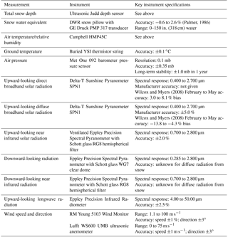
Table 3List of measurements and instruments used in this dataset at Mammoth Pass.
3.1.3 Radiation measurements
At CUES, uplooking broadband solar radiation, both diffuse and direct, is provided in this dataset by the Sunshine Pyranometer SPN-1. Incoming longwave radiation is measured via an Eppley Precision Infrared Radiometer (PIR). The broadband and near-infrared (nIR) snow albedos are measured using uplooking and downlooking radiometer pairs, with the downlooking radiometers on a fixed boom prior to September 2016 and on an adjustable boom thereafter.
3.2 Energy balance filtering
3.2.1 Air temperature, relative humidity, ground temperature, and air pressure filtering
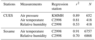
Air temperature, relative humidity, ground temperature, and air pressure were the simplest variables to process. Hourly averages were queried from the database containing measurements at 1 min temporal resolution. Visual examination of plots of these data revealed a few out-of-bounds measurements that were set to missing values. As with all the measurements, there were gaps of an hour to a few weeks, mostly in the summer, when instruments were removed for calibration or had failed. We arbitrarily chose a gap threshold of 12 h, and then used three approaches for gap-filling. For gaps below the gap threshold, a spline interpolation was performed. For gaps at or above the threshold, measurements were preferentially filled using a regression from two nearby sites with long-term measurements. All of the gaps in the air temperature, relative humidity, and air pressure were filled using these two methods. For air temperature and relative humidity, a site in the town of Mammoth Lakes was used as the other sensors on Mammoth Mountain suffered data losses during the same time periods at CUES/Sesame and MHP does not have a relative humidity sensor. The site is C2998, its station ID on Mesowest (http://mesowest.utah.edu, Horel et al., 2002). A regression for the matching times at each site was developed for both air temperature and relative humidity, with r2 values ranging from 0.53 to 0.91 (Table 4). The C2998 station did not have reliable pressure readings, so a regression from the local airport, called KMMH on Mesowest, was used (Table 4). Air temperature and relative humidity from KMMH were not used to gap fill as the airport is located in a rain shadow and in a flat valley with cold air pooling. These characteristics did not affect the air pressure as much, as the r2 value for the air pressure regression was 0.91. Because of the operational nature of the Sesame site, there were many more gaps that needed to be filled (N=6758–6868) compared to gaps at CUES (N=418–652). For ground temperature, the longer gaps had to be filled with climatology, given no other nearby measurements, while the gaps < 12 h were interpolated.
3.2.2 Wind speed and direction filtering
Wind speed and direction were queried from the database as average hourly values from 1 min samples. The Yamartino (1984) approach was used to average wind directions, consistent with the 1 min averaging that takes places on the data loggers with the raw measurements. CUES has three different wind sensors, but only the RM Young 5103 and the Lufft WS600-UMB provide reliable 1 min averages (Table 2). The RM Young 5103 and the WS600 are about 2 m apart in height, with the 5103 being at the platform height of about 6 m above the bare ground. The WS600 is mounted higher, about 3 m above the platform surface. Both of the wind sensors had periods of missing data or high readings, e.g., > 60 m s−1 for an hourly average. Thus, the RM Young 5103 values were preferentially used, with the WS600 measurements used to fill gaps using simple replacement. After this step, there were some small remaining gaps that were interpolated with a spline or filled with climatology using the same 12 h gap threshold. The measurement instrument and type of processing (i.e., measured, interpolated, or climatology) are recorded in the data table.
3.2.3 Uplooking radiation filtering
The direct B↓ and diffuse D↓ broadband radiations were queried from the database as average hourly values from 1 min samples. Direct broadband radiation values where transmittance T was above 0.95 were adjusted such that T=0.95 on the assumption that the absolute measurement errors for direct radiation are greater than for diffuse radiation.
where θ0 is the solar zenith angle, S=1367 W m−2 is the solar constant and Rv is the radius vector. These values can all be determined using location, date/time, and Ephemeris estimates, e.g., from the National Oceanic and Atmospheric Administration's Solar Calculator (https://www.esrl.noaa.gov/gmd/grad/solcalc/).
Periods of time with missing uplooking radiation were filled in with radiation from the nearby Dana Meadows, California Data Exchange Center (California Department of Water Resources, 2018), code DAN, at 37.897∘ N, 119.257∘ W at 2987 m. Comparisons of total solar radiation from CUES and DAN show decent though not excellent agreement, r2=0.85, RMSE = 133 W m−2. When DAN was the incoming solar radiation source, direct and diffuse components were estimated using an empirical method (Erbs et al., 1982) with a high-altitude modification (Olyphant, 1984). The uplooking SPN-1 is heated, so snow covering the radiometer was not observed, but the DAN radiometer is not heated. Without reliable co-incident downlooking measurements, it is difficult to flag these snow-covered periods, but we suggest that any snow cover on the radiometer is a minor issue given that DAN measurements during snowfall only comprise 0.26 % of the hourly uplooking measurements. Finally, there were a few periods left when neither CUES nor DAN had working uplooking broadband radiometers. These periods were multiple days in length, so climatology was used to estimate the incoming solar radiation. After plotting the gap-free dataset, there were some obvious spikes at night or around sunrise/sunset; therefore, all uplooking solar measurements are set to zero when cos θ0≤0; that is when the Sun was below the horizon. This will zero out some of the low-energy diffuse radiation at these times, but they are so small as to be insignificant to the energy balance.
The uplooking longwave radiation was relatively error free and required almost no filtering. There were gaps in the measurement record however that were filled using an empirical approach (Marks and Dozier, 1979) based on air temperature, and relative humidity when these ancillary measurements were available. We note that this approach is optimal for clear skies and produces low biased values, but it was only used for < 1 % of the uplooking longwave measurements. If these ancillary measurements were not available, climatology was used.
Table 4Gap-filling regression statistics. Shown are the stations with each of their measurements (“Stations”); measurements; the station that supplied the independent variable for the regression (“Regression station”); the r2 value of the regression; and the number of missing measurements filled using the regression (N).
3.2.4 Snow albedo filtering
The snow albedo estimates were by far the most complicated to process. In summary, snow albedo was calculated by (1) measuring the snow surface slope and aspect with a lidar; (2) using those slope and aspect measurements along with uplooking and downlooking radiometer measurements to create terrain-corrected direct broadband and near-infrared albedo measurements on clear days around solar noon; (3) bias correcting those observed albedos using theoretical maximums by season to account for different sensor configurations and other biases; (4) inverting the broadband and near-infrared albedos to estimate grain size and impurity content using a radiative transfer model; (5) interpolating the grain size and impurity content across non-clear days; and (6) creating an hourly direct broadband albedo, accounting for the solar geometry using the same radiative transfer model, run as a forward model.
For snow albedo measurement at CUES, there are four downlooking radiometers: a clear and nIR Eppley PSP on a fixed boom, and a clear and nIR Eppley PSP on an adjustable boom. In theory, these measurements can be used in conjunction with the uplooking radiometers to measure snow albedo. In practice, there are many biases and steps that need to be taken to obtain accurate measurements. Potential sources of error include a sloped snow surface such that the level uplooking radiometers do not receive the same amount of solar radiation as the snow; shadows cast by trees or other objects that can affect the uplooking and downlooking radiometers at different times; non-snow objects in the radiometers' field of view; an inability of the downlooking radiometers to distinguish diffuse radiation from the sky from that from the snow; direct solar radiation reaching the downlooking radiometers at high solar zenith angles; and imperfect cosine response and other instrument biases in the radiometers (Wilcox and Myers, 2008), especially at the higher solar zenith angles. To address the issue of non-snow objects in the downlooking radiometers' field of view, an adjustable boom was installed in September 2015. The boom is kept about 1 m above the snow surface to eliminate non-snow objects from the radiometers' field of view. Thus, for water years 2016 and 2017, the adjustable downlooking boom measurements were used, while for all other years, only the fixed boom downlooking measurements could be used. We could not find a good relationship between the fixed boom and downlooking boom radiation values to correct the prior years. Instead, we used a bias correction based on the maximum observed annual albedo, explained below.
Because of the issue of not being able to discriminate diffuse radiation from the sky versus diffusion radiation from the snow and problems with measurements at high solar zenith angles, albedo measurements were only used 1 time a day during clear-sky conditions, , around solar noon. In addition, to eliminate problems with shadows, only the maximum downlooking daily values were retrieved. Thus, the database was queried to find the maximum daily downlooking broadband radiation values during clear-sky conditions and to return the associated time, uplooking broadband/nIR measurement, and downlooking nIR measurement. Queries were further restricted to times when at least 30 cm of snow was measured on the ground and direct solar radiation was > 400 W m−2 to ensure that only sunny days with broad snow cover were selected. The uplooking direct and nIR measurements were then corrected to the snow surface using a correction factor c (Bair et al., 2015; Painter et al., 2012):
with θ as the local solar illumination angle such that the albedo α is the ratio of the reflected solar radiation D↑ and the terrain-corrected direct and diffuse solar radiation, with the diffuse being uncorrected assuming a negligible terrain effect on it:
For the uplooking near-infrared measurements, the diffuse fraction was not known, so we assumed that all of the radiation was direct based on atmospheric scattering being small at these wavelengths.
To compute θ, the slope and aspect of the snow surface must be measured. To do this we used a Reigl Z390i laser scanner that operates automatically on a schedule at CUES that has varied over the study period from every 15 min to every hour. A point cloud from the scan nearest the albedo acquisition was selected. Then, a 2 m2 bounding box within both the fixed and adjustable downlooking radiometers' fields of view was used to filter this point cloud. This filtered point cloud was then fit with a plane to determine the local slope and aspect. There were periods when the laser scanner was not working properly or times prior to its installation in February 2011. For these times, the modal aspect (north) and slope (4∘) were used for the terrain correction. Because the albedos were measured near solar noon and the slope of the terrain is low, c is significantly less than 1 only during times when θ0 is high; those are times around solar noon during the accumulation season. From mid-April through melt-out, c is close to 1, making the terrain correction negligible.
From the corrected albedos, for each season, the maximum value for that season was compared with a theoretical maximum of 0.89 for a broadband albedo and 0.74 for an nIR albedo (Dozier et al., 2009). Values were then adjusted up or down by the difference between the observed and theoretical maxima on an annual basis. The average annual correction was +5.1 % for the broadband albedo and −3.9 % for the nIR albedo. These values suggest that trees, which are darker in the visible spectrum but brighter than coarse grained dirty snow in the nIR, were often in the downlooking radiometers' field of view, especially later in the season. A minimum theoretical albedo was not used for correction as this will vary from season to season (e.g., Painter et al., 2012) depending on the concentration of impurities on the surface of the snowpack.
The assumption behind our maximum albedo correction is that the annual calibration or swapping of some of the instruments that occurs at CUES each fall could explain the bias, and that this bias is scalar in nature. The latter assumption is unlikely to be true, but we decided it was the best correction given the documented radiometer biases (Wilcox and Myers, 2008). We note that WY 2017 required a negligible correction since the adjustable downlooking boom was used. Curiously, albedos from WY2016 required a negative correction even though this was the first year that the adjustable downlooking boom was installed. Our explanation is that between WY 2016 and WY 2017 the downlooking boom design changed such that aluminum from the downlooking boom was visible to the radiometers on the downlooking boom in 2016 but not in 2017. Reflected light from the aluminum boom caused the downlooking radiometers to have high biased measurements. Also, we note that the spectral range of the SPN-1 and the PSP are different, 0.400 to 2.700 vs. 0.285 to 2.800 µm (Table 2); however, because of different documented biases (Wilcox and Myers, 2008), especially at higher solar zenith angles, the SPN-1 shows 2.5 % more broadband radiation on average than the PSP. This sort of unanticipated bias further supports our approach of using a theoretical maximum albedo to bias correct our measurements.
For the times when the uplooking radiometers at CUES were not working, albedos were estimated using a multivariate regression based on time since last snowfall (of at least 2.54 cm/1 inch) and θ. This approach showed similar accuracy to what was expected from a simple statistical model based only on snowfall and solar geometry, r2=0.62, RMSE = 7.0 %. Other variables such as new snow density and total snow depth were added to the regression but did not improve its accuracy. We note that this RSME value is only slightly larger than the average annual bias correction of 5.1 %, illustrating the uncertainties associated with in situ snow albedo measurement.
From these broadband and near-infrared albedos, the grain size and impurity content of the snowpack were estimated using a two-stream radiative transfer model where grain size and impurity content are solved simultaneously using nonlinear optimization (Meador and Weaver, 1980; Moré, 1977). The grain sizes and impurity content were then interpolated from the daily to hourly times across the study period. This grain size interpolation likely overestimates grain sizes on days with new snowfall that were cloudy, as no albedo measurements were taken on these days. One approach would be to use a constant value for new snow albedo, which is done for age-based models (e.g., Dickinson et al., 1993; U.S. Army Corps of Engineers, 1956); however, on the days with new snowfall of greater than 2.54 cm/1 in. that were sunny and therefore had albedo measurements around solar noon, there was substantial scatter in the new snow albedo, ranging from 0.60 to 0.89, illustrating the pitfalls of using a constant new snow albedo.
The interpolated grain sizes and impurity content were then fed back into the model varying by θ0 with each hour as the solar zenith changed. The assumptions of this approach are that (1) the grain size changes relatively less than the albedo throughout the diurnal cycle; and (2) the daily albedo cycle is more accurately modeled than measured, which is based on our experience at CUES. Assumption (1) is the weaker assumption as grain size decay or growth can be rapid in the first day or two after snowfall (Flanner and Zender, 2006), but for snow that is older than a day or two, which is most melting snow, the assumption is reasonable.
3.3 Mass balance
3.3.1 Automated snow depth/SWE and manual precipitation measurements
The mass balance measurements come from all three sites. We provide snow depth from ultrasonic sensors at each site over the entire period of record. We also provide snow pillow measurements for all three sites, but only over the entire period of record at MHP. At CUES, the snow pillow measurements start with the installation of the pillow in September 2012 and are provided continuously through September 2017. At Sesame, snow pillow measurements start in October 2013 and are provided continuously up until February 2017, when the pressure transducer failed. At CUES and Sesame, the ultrasonic depth sensors are located directly above the snow pillows. At MHP, the depth sensor is mounted on a boom adjacent to the pillow. Heated tipping bucket measurements were taken at Sesame and MHP over the entire period of record; however, only the MHP tipping bucket measurements are provided because of gaps and quality problems with the Sesame gauges discussed in Sect. 2.1. The MHP tipping bucket measurements were not without problems, including undercatch, data gaps, and spurious precipitation during times when it was not precipitating. These problems are discussed below.
3.3.2 Automated snow depth/SWE and manual precipitation measurement filtering
The snow depth measurements from the ultrasonic depth sensors at all three sites required extensive filtering and interpolation, which is common. For the Sesame site, the raw depth measurements were taken every minute. At CUES, the depth measurements were taken every 15 min from October 2010 until September 2012. From September 2012 onwards, the depth measurements were taken every 5 min. All of these depth readings are actually averages, as each depth pinger samples at once a minute or more frequently. At MHP, depth measurements are only available hourly, also presumably as averages rather than instantaneous measurements.
Ultrasonic snow depth measurements suffer from both drops and spikes, but spikes are more prevalent, especially at CUES, where blowing snow can reflect the sound, thereby causing the snowpack to appear to be at or near the sensor height. Thus, the aggregation used the minimum depth at CUES and Sesame over each hour to limit spikes. The aggregated data were then plotted and inspected visually. First, snow-free periods were identified manually based on visual inspection of the measurements and ancillary knowledge of the snow accumulation season, e.g., Sesame manual measurements. These manually identified periods were set to zero depth. Likewise, a snow-covered period was created as the opposite of the snow-free period. Values of zero during snow cover were set to a missing value. Other large spikes over extended periods of time, such as during sensor maintenance, were set to a missing value. An outlier filter (Hampel, 1974) was used to reduce spikes and drops further. Missing values were then interpolated using a shape-preserving piecewise cubic spline. The interpolated data were then smoothed using a smoothing spline to reduce high-frequency noise. This method tended to produce very small values (≪ 0.1 cm) rather than zeros at times. These small values were set to zero.
The snow pillow measurements at all three sites were quite clean in comparison to the snow depth measurements. The same snow-free periods used for the depth sensors were used to set the pillows to zero, usually to eliminate high-frequency noise during the snow-free season. Likewise, values of zero during snow cover were set to a missing value. Missing values were interpolated also using cubic splines. High-frequency noise was smoothed with a spline and values < 0.6 cm were set to zero.
Measurements from the heated tipping bucket at MHP showed many problems. They were given as accumulated precipitation over the water year and converted to hourly precipitation intensity values using a forward-looking difference. There were many time gaps with missing measurements, possibly because the modem could not transmit or because of power losses to the sensor or its heater. In the case of a gap, any increase in precipitation since the last measurement time was interpolated linearly across the length of the gap. This approach assumes a data transmission failure where the logger provides the correct accumulated precipitation value after the gap. Then, there were five measurements with rates above the maximum rate Pmax, assumed to be 1 in./2.54 cm per hour, based on our experience with measuring precipitation at Sesame. We assumed these were due to clogging of the orifice or a heater failure; thus, we spread the high values Phi out over N hours such that the precipitation rate Pt at time t is
Comparison of the hourly Sesame heated tipping bucket precipitation during times when the tipping bucket was working (approx. November–May, 2013–2017) and the hourly MHP heated tipping bucket measurements shows a low r2=0.08, although accumulated precipitation was closer, with Sesame showing 92 % of the accumulated precipitation of MHP. Further analysis shows many times when the Met One tipping bucket was not recording precipitation but the MHP precipitation bucket was recording small values (0.1 cm). Given that we are more confident in the limited tipping bucket measurements from Sesame based on our experience with the site, we suggest that there was a heater problem at MHP that caused the tipping bucket there to accumulate snow during storms and melt it afterwards. Because of the above problems, we caution against using the MHP tipping bucket measurements for hourly precipitation, as they are more accurate for accumulated sums over longer time periods.
The manual Sesame measurements were checked visually for errors and edited to be consistent from year to year and adjusted to conform to operational standards (American Avalanche Association, 2016), but no major adjustments were made. We have kept the measurements in Imperial units to preserve how they were taken and how the notes refer to the measurements. Minor adjustments included altering the table to show “Trace” amounts of new snow in a consistent way and some formatting changes. For example, null or blank values that were not applicable such as new snow density on days with rain only were converted to “NaN” (not a number). Also, we note that the reported “density” is not sampled from the snowpack, but is simply a measure of the weighed SWE/height of new snow. Given mixed precipitation, the SWE measurements sometimes contain liquid water leading to high densities, e.g., 90 % on 19 October 2015. Also, snow is only recorded to the nearest 0.5 in., which for small snowfall events can also led to unrealistic densities due to the lack of measurement precision.
As mentioned several times, CUES is the only site where the full energy and mass balance is measured on Mammoth Mountain; therefore, it is ideal for a full mass/energy balance simulation. Because precipitation measurements at CUES are uncertain, we ran the SNOWPACK model under three different precipitation forcings: (a) hourly tipping bucket precipitation measurements from MHP with a rain–snow discrimination based on wet bulb temperature; (b) snow depth from CUES using the empirical new snow density model in SNOWPACK; (c) all available information. For each of the model runs, the period from September 2012 to September 2017 was used to match times when snow pillow measurements of SWE are available from CUES. The following measurements were provided to SNOWPACK: upward-looking broadband solar radiation; ground temperature (just beneath the snow–soil interface); uplooking longwave radiation; air temperature; relative humidity; wind speed; and reflected radiation (albedo × upward-looking broadband). The model was run at a 15 min time step with hourly outputs. Neutral stability was assumed given the moderate to high wind speeds at CUES, an assumption made for similar sub-alpine environments (Lehning et al., 2002; Mitterer and Schweizer, 2013). Other parameters shared among model runs were left at default values.
4.1 Model run using hourly tipping bucket precipitation (a)
In addition to the hourly precipitation, we elected to provide the solid precipitation percentage using an empirical wet bulb formula from over 9700 stations (Sims and Liu, 2015). The other option would have been to use the default air temperature based rain–snow discriminator (1.2 ∘C) in SNOWPACK, which has been shown to be a less accurate discriminator than the wet bulb temperature (Sims and Liu, 2015).
4.2 Model run using hourly snow depth only (b)
For this model run, we relied on an empirical new snow density relationship computed by SNOWPACK (Zwart, 2007) which uses air temperature, relative humidity, and wind speed. Using snow depth only is in fact the way SNOWPACK was designed to be run for the IMIS weather stations in Switzerland, which like CUES, have snow depth (although not SWE) sensors but not precipitation gauges because of wind-related problems (Lehning et al., 2002).
4.3 Model run using all available information (c)
In this model run, we combined the changes in hourly snow depth with measured new snow density to derive a precipitation rate. The forward-looking difference in snow depth was computed. Then, for all positive changes in snow depth, a manually measured new snow density from the nearest time was applied, i.e., nearest neighbor interpolation of densities. We also accounted for rainfall by adding tipping bucket measurements from MHP during times when the snow depth was not increasing but the tipping bucket was recording precipitation. Solid precipitation percentage was supplied as in (a).
We have selected five different measurement areas for comparison: snow depth and air temperatures at Sesame and CUES; albedo cycle at CUES; wind climatology at CUES; and uplooking longwave radiation at CUES. Then, we compare the mass balance predictions from the three model runs against our measured SWE at CUES.
5.1 Data comparison
5.1.1 Snow depth
Overall, the snow depth at both sites agrees well (Fig. 5), with CUES having a later melt-out date, explained by its higher elevation and slightly north-facing terrain, while Sesame had slightly greater snow depths in the wet years, i.e., 2011 and 2017, possibly because the snow under the depth sensor at CUES was removed by wind transport during the big storms.
The 2011 to 2017 water years show a tremendous diversity in snow accumulation. At Sesame, where precipitation records go back to the 1983 water year, 2017 was the wettest year on record, with 255 cm of precipitation, while 2015, with 55 cm of precipitation, was the driest. We stress that the measurements from Sesame do not cover the entire water year and do not always cover consistent time periods from year to year, depending on when the ski resort opened and closed. An examination of the nearby MHP snow course, with records back to 1928, shows 2 years with greater maximum SWE on the ground: 220 cm of SWE on 27 March 1969 and 216 cm on 25 April 1983. Water year 2017 was third, with 208 cm of SWE on the ground on 31 March 2017. There are no reliable precipitation gauges with record lengths > 40 years in the area around Mammoth Mountain. The closest is Huntington Lake, lower at 2134 m elevation, where 2017 ranks fifth among water years going back to 1912.
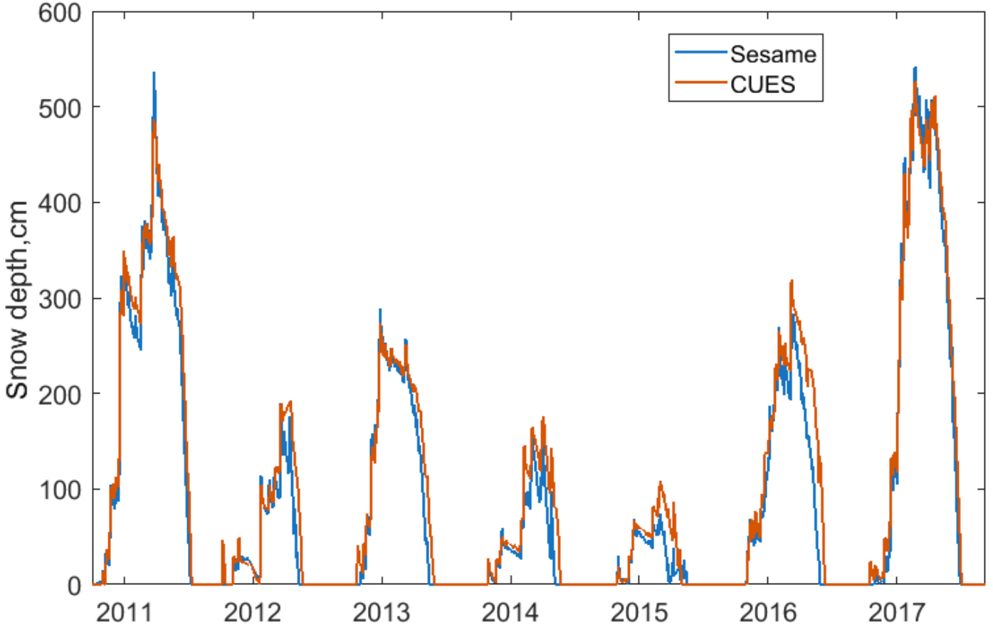
Figure 5Snow depth at Sesame and at CUES during the study period. Note the similar depths with slightly later melt-out at CUES, especially in the drier years.
In terms of maximum snow depth, 2015 was the lowest on record, with 75 cm at Sesame and 112 cm at CUES. Despite having the most precipitation, water year 2017, with peak snow depths of 526 cm at Sesame and 543 cm at CUES, did not have the deepest snow depths recorded at either site. At Sesame, 2006, with a 610 cm peak snow depth, and 1995 with a 561 cm peak snow depth, both had more snow on the ground than 2017. At CUES, reliable snow depths only go back to 2001, but snow depth was over 600 cm in 2006 when the downlooking boom was buried. Subsequently, it was raised up to the top of the railing from the platform floor.
5.1.2 Air temperature
The Sesame site is slightly warmer than CUES, with an average annual temperature of 4.88 ∘C vs. 4.50 ∘C, although the November through May temperatures, which correspond to the average period when snow is on the ground, are equivalent to within the instrument uncertainty with both sites at −0.11 ∘C. Comparing midwinter temperatures at both sites (Fig. 6), we see that above-freezing temperatures are common and that the diurnal range is considerably narrower at CUES, which follows given its mid-mountain and exposed location in comparison to Sesame's location near a valley, with Seame subject to longwave heating from the trees and cold air pooling at night.
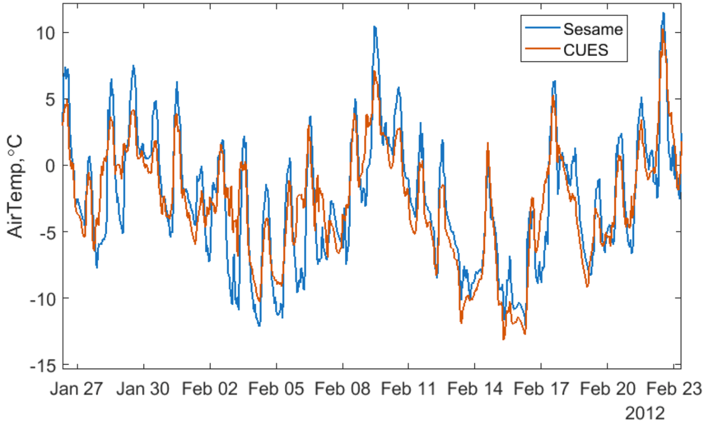
Figure 6Air temperature at Sesame and at CUES during a selected midwinter period. Note the greater diurnal range for Sesame.
5.1.3 Albedo
The broadband snow albedo at CUES is usually above 0.80 for much of the accumulation season, with values reaching above 0.90 for the highest solar zenith angles. When the albedo stops being refreshed by new snow and the old snow is covered with pumice, the albedo drops dramatically. In every season, minimum albedo values were < 0.60. A large diurnal variation in albedo of > 20 % is evident for days late in the melt season due to the range of solar zenith angles (Fig. 7). Although there is little energy reaching the snowpack in the early morning and late afternoon, when the solar zenith angles and albedo are highest, the illumination angle effect on albedo is significant and should be included in all snowmelt models nonetheless.

Figure 7Diurnal variation in albedo for a day in June 2017. Note the large range, although the solar energy reaches the snowpack at the times when the highest albedo is low.
5.1.4 Wind
A wind rose for CUES (Fig. 8) shows wind speeds in the range of previously published measurements from an anemometer mounted on top of Main Lodge (Bair, 2013). As with all mountain areas, there is substantial variability in the wind speed. For example, the average ridge top wind speeds are at least 50 % greater than these (Bair, 2011) and the highest reliably recorded wind gust from the top of Mammoth Mountain was measured at 82.3 m s−1.
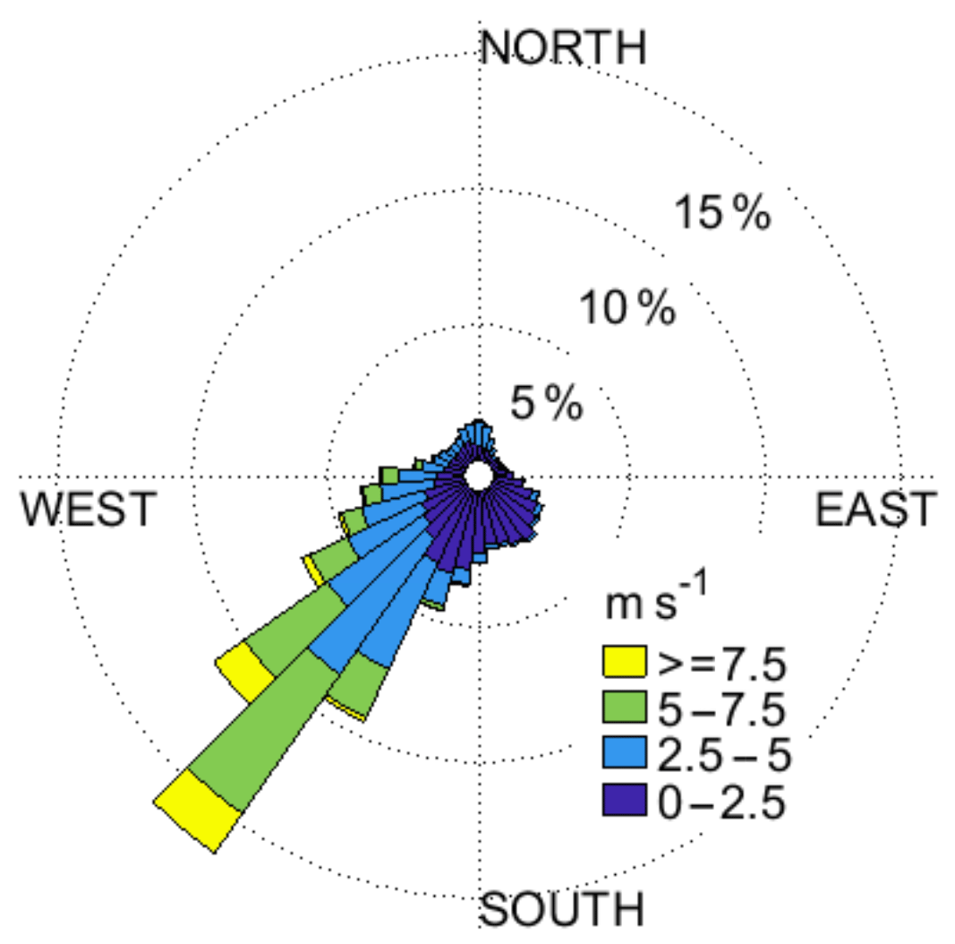
Figure 8Wind rose for CUES, a windy site. Hourly values are plotted. Note the predominant southwest wind direction.
5.1.5 Uplooking longwave radiation
To illustrate the importance of measuring incoming longwave radiation rather than modeling it using the more commonly available temperature and relative humidity measurements, we have plotted modeled values against measured values for clear-sky conditions during the day (Fig. 9). The model (Marks and Dozier, 1979) is optimal for clear-sky conditions, with clear conditions defined the same as for direct albedo measurement: . There is a strong negative bias of −40 W m−2 or −17 % of the mean measured value. The RMSE of 43 W m−2 is within the ranges reported in Marks and Dozier (1979), and they also report a similar negative bias.
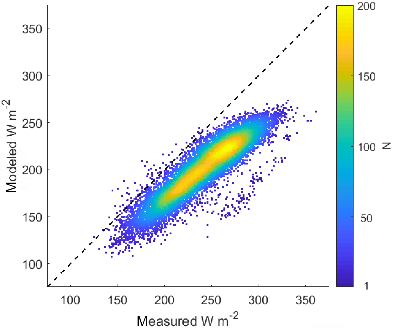
Figure 9Density plot of modeled vs. measured uplooking longwave radiation for clear-sky measurements. The number of measurements N is represented by the color scale. Note the clear negative model bias.
5.2 Snow mass balance simulation using SNOWPACK
The modeled versus measured SWE (Fig. 10) was clearly closest for model run b (snow depth only). Mean errors (modeled–measured) were −25.5, −1.7, and −11.3 cm for model runs a–c. All the runs underestimated SWE on average; however, the direction of the bias for model runs b and c (all available information) depended on the year, while model run a (MHP precipitation) was low biased for all years. Model runs a and c were much lower biased than model run b, so we discuss possible explanations for the bias in those two runs first.
SWE was severely underestimated by the tipping bucket at MHP, which is not surprising given how much more snow accumulates on the snow pillow at CUES than at MHP, 128 vs. 82 cm for the 2013 to 2017 average annual maximum, as well as the timing problems with the MHP tipping bucket measurements (Sect. 3.3.2). The greater accumulation at CUES is almost entirely due to wind redistribution, as the pillow sits just past a cluster of trees that act as a snow fence, causing deceleration of the wind and increased deposition (Tabler, 1980). Since model run c used snow depth measured directly above the pillow, one might have expected it to perform similarly to model run b where only depth was used. We suggest that differences in the new snow density models can explain most of the difference. Essentially, the new snow density was underestimated by using the manual measurements at Sesame because that site is subject to much lower wind speeds than CUES. Winds fragment snow crystals (Fierz et al., 2009; Seligman, 1936) so that they pack more tightly, causing higher density new snow. Wind speed is accounted for in the empirical new snow density model used by SNOWPACK (Zwart, 2007), but the manual density measurements made at CUES do not account for this wind packing effect. We suggest this is the main reason for the much more negative bias in model run c than in model run b. Had we used Sesame as the target site for the model runs, we speculate that model run c would have produced excellent agreement with the pillow measurements. However, we lack the radiation measurements needed to force a full energy balance model at Sesame.

Figure 10Modeled vs. measured SWE at CUES using three different precipitation forcings: (a) tipping bucket precipitation from MHP with wet bulb temperature solid precipitation percentage; (b) snow depth only from CUES; (c) all available information.
The low bias overall by both model runs b and c and the changing sign of the bias are more difficult to explain. Often the rain snow line is just above Sesame, but below CUES, so it is possible that density is overestimated sometimes by the manual measurements at Sesame during mixed rain–snow events. Likewise, the Zwart (2007) density model by SNOWPACK has inherent errors, which is why SNOWPACK offers five different new snow density models.
These data are available at http://www.snow.ucsb.edu with https://doi.org/10.21424/R4159Q (Bair et al., 2018). They consist of four large comma-separated tables, uncompressed in ASCII format with one-line headers. The tables are the daily Sesame Snow Study Plot manual precipitation and weather with notes; the hourly Sesame Snow Study Plot air temperature, relative humidity, snow depth, and SWE; the CUES hourly radiation, snow albedo, wind speed, air temperature, ground temperature, relative humidity, air pressure, snow depth, and SWE; and the hourly Mammoth Pass precipitation, snow depth, and SWE.
In order to provide hourly mass and energy balance measurements that can be used to test and validate snow models, we have created a carefully filtered dataset using instruments at three sites on Mammoth Mountain, CA. We then tested these measurements in a snow model to estimate snowpack mass balance. The model run using measured snow depth only from CUES matched the measured SWE from the snow pillow there very well with a −1.7 cm bias on average. These years comprise the wettest year since 1983 and the driest year on record. Unique measurements include hand-weighed daily snow measurements from the Sesame Snow Study Plot and terrain-corrected broadband snow albedo. This dataset only comprises a fraction of the measurements available on Mammoth Mountain. We encourage interested researchers to explore the raw measurements available on the CUES website at http://www.snow.ucsb.edu if this dataset does not meet their modeling needs.
The supplement related to this article is available online at: https://doi.org/10.5194/essd-10-549-2018-supplement.
EHB performed most of the data production, analysis, and authoring of the manuscript. JD wrote the radiative transfer incoming solar filtering code. He and RED, who both edited the manuscript, have kept CUES funded and running in its current location for almost 30 years.
The authors declare that they have no conflict of interest.
This article is part of the special issue “Hydrometeorological data from mountain and alpine research catchments”. It is not associated with a conference.
We thank three anonymous reviewers for their critical insights. This work
was supported by NASA awards NNX12AJ87G and NNX15AT01G and U.S. Army Cold
Regions Research and Engineering Laboratory award W913E5-16-C-0013.
Edited by: Danny Marks
Reviewed by: three anonymous referees
American Avalanche Association: Snow, Weather, and Avalanches: Observational Guidelines for Avalanche Programs in the United States, 3rd ed., American Avalanche Association, Victor, ID, 104 pp., 2016.
Bailey, R. A.: Geologic map of Long Valley caldera, Mono-Inyo Craters volcanic chain, and vicinity, eastern California, US Geological Survey Map I-1933, 62000, 1989.
Bair, E. H.: Fracture mechanical and statistical properties of nonpersistent snow avalanches, Ph.D. Thesis, Donald Bren School of Environmental Science and Management, University of California (available at: https://www.eri.ucsb.edu/people/ned-bair), Santa Barbara, CA, 183 pp., 2011.
Bair, E. H.: Forecasting artificially-triggered avalanches in storm snow at a large ski area, Cold Reg. Sci. Technol., 85, 261–269, https://doi.org/10.1016/j.coldregions.2012.10.003, 2013.
Bair, E. H., Dozier, J., Davis, R. E., Colee, M. T., and Claffey, K. J.: CUES – A study site for measuring snowpack energy balance in the Sierra Nevada, Front. Earth Sci., 3, 58, https://doi.org/10.3389/feart.2015.00058, 2015.
Bair, E. H., Davis, R. E., and Dozier, J.: Supplement to Hourly mass and snow energy balance measurements from Mammoth Mountain, available at: https://doi.org/10.21424/R4159Q, last access: March 2018.
Bales, R. C., Molotch, N. P., Painter, T. H., Dettinger, M. D., Rice, R., and Dozier, J.: Mountain hydrology of the western United States, Water Resour. Res., 42, W08432, https://doi.org/10.1029/2005WR004387, 2006.
Barnett, T. P., Adam, J. C., and Lettenmaier, D. P.: Potential impacts of a warming climate on water availability in snow-dominated regions, Nature, 438, 303–309, https://doi.org/10.1038/nature04141, 2005.
California Department of Water Resources: California Data Exchange Center, available at: http://cdec.water.ca.gov/ (last access: February 2018), 2018.
Dickinson, R. E., Henderson-Sellers, A., and Kennedy, P. J.: Biosphere-Atmosphere Transfer Scheme (BATS) Version 1e as coupled to the NCAR Community Climate Model, National Center for Atmospheric Research, Boulder, Colorado, Technical Note NCAR/TN-387+STR, 72, 1993.
Dozier, J., Green, R. O., Nolin, A. W., and Painter, T. H.: Interpretation of snow properties from imaging spectrometry, Remote Sens. Environ., 113, S25–S37, https://doi.org/10.1016/j.rse.2007.07.029, 2009.
Erbs, D. G., Klein, S. A., and Duffie, J. A.: Estimation of the diffuse radiation fraction for hourly, daily and monthly-average global radiation, Solar Energy, 28, 293–302, https://doi.org/10.1016/0038-092X(82)90302-4, 1982.
Fierz, C., Armstrong, R. L., Durand, Y., Etchevers, P., Greene, E., McClung, D. M., Nishimura, K., Satyawali, P. K., and Sokratov, S.: The International Classification for Seasonal Snow on the Ground, IHP-VII Technical Documents in Hydrology N∘83, 90, 2009.
Flanner, M. G. and Zender, C. S.: Linking snowpack microphysics and albedo evolution, J. Geophys. Res., 111, D12208, https://doi.org/10.1029/2005JD006834, 2006.
Goodison, B., Louie, P. Y. T., and Yang, D.: WMO Solid precipitation measurement intercomparison, World Meteorological Organization, 1998.
Hampel, F. R.: The Influence Curve and its Role in Robust Estimation, J. Am. Stat. Assoc., 69, 383–393, https://doi.org/10.1080/01621459.1974.10482962, 1974.
Hildreth, W.: Volcanological perspectives on Long Valley, Mammoth Mountain, and Mono Craters: Several contiguous but discrete systems, J. Volcanol. Geotherm. Res., 136, 169–198, https://doi.org/10.1016/j.jvolgeores.2004.05.019, 2004.
Horel, J., Splitt, M., Dunn, L., Pechmann, J., White, B., Ciliberti, C., Lazarus, S., Slemmer, J., Zaff, D., and Burks, J.: Mesowest: Cooperative Mesonets in the Western United States, B. Am. Meteorol. Soc., 83, 211–225, https://doi.org/10.1175/1520-0477(2002)083<0211:mcmitw>2.3.co;2, 2002.
Landry, C. C., Buck, K. A., Raleigh, M. S., and Clark, M. P.: Mountain system monitoring at Senator Beck Basin, San Juan Mountains, Colorado: A new integrative data source to develop and evaluate models of snow and hydrologic processes, Water Resour. Res., 50, 1773–1788, https://doi.org/10.1002/2013WR013711, 2014.
Lehning, M., Bartelt, P., Brown, B., and Fierz, C.: A physical SNOWPACK model for the Swiss avalanche warning: Part III: meteorological forcing, thin layer formation and evaluation, Cold Reg. Sci. Technol., 35, 169–184, https://doi.org/10.1016/S0165-232X(02)00072-1, 2002.
Löffler-Mang, M., Kunz, M., and Schmid, W.: On the Performance of a Low-Cost K-Band Doppler Radar for Quantitative Rain Measurements, J. Atmos. Ocean. Technol., 16, 379–387, https://doi.org/10.1175/1520-0426(1999)016<0379:OTPOAL>2.0.CO;2, 1999.
Marks, D. and Dozier, J.: A clear-sky longwave radiation model for remote alpine areas, Theor. Appl. Climatol., 27, 159–187, https://doi.org/10.1007/BF02243741, 1979.
Marks, D. and Dozier, J.: Climate and energy exchange at the snow surface in the alpine region of the Sierra Nevada, 2, Snow cover energy balance, Water Resour. Res., 28, 3043–3054, https://doi.org/10.1029/92WR01483, 1992.
Matrosov, S. Y.: Modeling Backscatter Properties of Snowfall at Millimeter Wavelengths, J. Atmos. Sci., 64, 1727–1736, https://doi.org/10.1175/JAS3904.1, 2007.
Meador, W. E. and Weaver, W. R.: Two-stream approximations to radiative transfer in planetary atmospheres – A unified description of existing methods and a new improvement, J. Atmos. Sci., 37, 630–643, https://doi.org/10.1175/1520-0469(1980)037<0630:TSATRT>2.0.CO;2 1980.
Mitterer, C. and Schweizer, J.: Analysis of the snow-atmosphere energy balance during wet-snow instabilities and implications for avalanche prediction, The Cryosphere, 7, 205–216, https://doi.org/10.5194/tc-7-205-2013, 2013.
Moré, J. J.: The Levenberg-Marquardt algorithm: Implementation and theory, in: Numerical Analysis, edited by: Watson, G. A., Springer Verlag, Berlin, 105–116, 1977.
NOAA National Climatic Data Center: Climate at a Glance, Time Series data, available at: http://www.ncdc.noaa.gov/cag/ (last access: February 2018), 2018.
Olyphant, G. A.: Insolation topoclimates and potential ablation in alpine snow accumulation basins: Front Range, Colorado, Water Resour. Res., 20, 491–498, https://doi.org/10.1029/WR020i004p00491, 1984.
Painter, T. H., Skiles, S. M., Deems, J. S., Brandt, W. T., and Dozier, J.: Variation in Rising Limb of Colorado River Snowmelt Runoff Hydrograph Controlled by Dust Radiative Forcing in Snow, Geophys. Res. Lett., 45, 797–808, https://doi.org/10.1002/2017GL075826, 2018.
Painter, T. H., Skiles, S. M., Deems, J. S., Bryant, A. C., and Landry, C. C.: Dust radiative forcing in snow of the Upper Colorado River Basin: 1. A 6 year record of energy balance, radiation, and dust concentrations, Water Resour. Res., 48, W07521, https://doi.org/10.1029/2012WR011985, 2012.
Palmer, P. L.: Estimating snow course water equivalent from SNOTEL pillow telemetry: an analysis of accuracy, 54th Annual Western Snow Conference, Western Snow Conference, Phoenix, Arizona, 1986.
Reba, M. L., Link, T. E., Marks, D., and Pomeroy, J.: An assessment of corrections for eddy covariance measured turbulent fluxes over snow in mountain environments, Water Resour. Res., 45, W00D38, https://doi.org/10.1029/2008WR007045, 2009.
Seligman, G.: Snow Structure and Ski Felds, MacMillan & Co., London, 1936.
Sims, E. M. and Liu, G.: A Parameterization of the Probability of Snow–Rain Transition, J. Hydrometeorol., 16, 1466–1477, https://doi.org/10.1175/JHM-D-14-0211.1, 2015.
Slaughter, C. W., Marks, D., Flerchinger, G. N., Van Vactor, S. S., and Burgess, M.: Thirty-five years of research data collection at the Reynolds Creek Experimental Watershed, Idaho, United States, Water Resour. Res., 37, 2819–2823, https://doi.org/10.1029/2001WR000413, 2001.
Sterle, K. M., McConnell, J. R., Dozier, J., Edwards, R., and Flanner, M. G.: Retention and radiative forcing of black carbon in eastern Sierra Nevada snow, The Cryosphere, 7, 365–374, https://doi.org/10.5194/tc-7-365-2013, 2013.
Tabler, R. D.: Geometry and density of drifts formed by snow fences, J. Glaciol., 26, 405–419, 1980.
U.S. Army Corps of Engineers: Snow Hydrology: Summary Report of the Snow Investigations, North Pacific Division, Corps of Engineers, Portland, OR, 462 pp., 1956.
van den Broeke, M. R., Smeets, C. J. P. P., and van de Wal, R. S. W.: The seasonal cycle and interannual variability of surface energy balance and melt in the ablation zone of the west Greenland ice sheet, The Cryosphere, 5, 377–390, https://doi.org/10.5194/tc-5-377-2011, 2011.
Wilcox, S. M. and Myers, D. R.: Evaluation of radiometers in full-time use at the National Renewable Energy Laboratory Solar Radiation Research Laboratory, National Renewable Energy Laboratory, Golden, CO USA, 45, 2008.
Yamartino, R. J.: A Comparison of Several “Single-Pass” Estimators of the Standard Deviation of Wind Direction, J. Clim. Appl. Meteorol., 23, 1362–1366, https://doi.org/10.1175/1520-0450(1984)023<1362:ACOSPE>2.0.CO;2, 1984.
Zwart, C.: Significance of new-snow properties for snowcover development, M.Sc. Thesis, University of Utrecht, 78 pp., 2007.