the Creative Commons Attribution 4.0 License.
the Creative Commons Attribution 4.0 License.
 | 28 Mar 2018
Construction of a surface air temperature series for Qingdao in China for the period 1899 to 2014
Yan Li
Birger Tinz
Hans von Storch
Qingyuan Wang
Qingliang Zhou
Yani Zhu
We present a homogenized surface air temperature (SAT) time series at 2 m height for the city of Qingdao in China from 1899 to 2014. This series is derived from three data sources: newly digitized and homogenized observations of the German National Meteorological Service from 1899 to 1913, homogenized observation data of the China Meteorological Administration (CMA) from 1961 to 2014 and a gridded dataset of Willmott and Matsuura (2012) in Delaware to fill the gap from 1914 to 1960. Based on this new series, long-term trends are described. The SAT in Qingdao has a significant warming trend of 0.11 ± 0.03 ∘C decade−1 during 1899–2014. The coldest period occurred during 1909–1918 and the warmest period occurred during 1999–2008. For the seasonal mean SAT, the most significant warming can be found in spring, followed by winter. The homogenized time series of Qingdao is provided and archived by the Deutscher Wetterdienst (DWD) web page under overseas stations of the Deutsche Seewarte (http://www.dwd.de/EN/ourservices/overseas_stations/ueberseedoku/doi_qingdao.html) in ASCII format. Users can also freely obtain a short description of the data at https://doi.org/https://dx.doi.org/10.5676/DWD/Qing_v1. And the data can be downloaded at http://dwd.de/EN/ourservices/overseas_stations/ueberseedoku/data_qingdao.txt.


Surface air temperature at 2 m (hereinafter referred to as SAT) is one of the most important climate elements influencing the biosphere and human activities. Systematical observations in China on a national scale started in 1951. However, the 60-year length of the SAT dataset seems insufficiently long to understand the long-term trend and interdecadal variability. For detecting changes beyond the range of natural variations (e.g., Zorita et al., 2008) and for attributing such a change to plausible drivers (a concept introduced by Hasselmann, 1979, known as “detection and attribution”), longer observational series are needed. Therefore, the changes in temperatures in China in the past more than 100 years need to be investigated in more detail (Qian and Zhu, 2001; Qian et al., 2011; Soon et al., 2011).
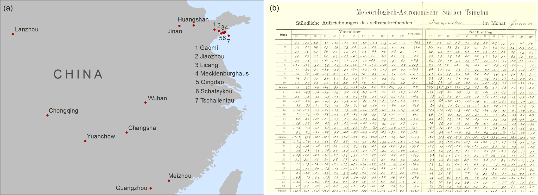
Figure 1Positions of the 14 stations of the German Marine Observatory in China (a); handwritten observations of Qingdao (b) from the archive of the German Meteorological Service in Hamburg, Germany.
Several annual mean SAT series for China commencing in the late 19th century have been constructed (Lin et al., 1995; Mitchell et al., 2002; Wang et al., 2004; Tang and Ren, 2005; Tang et al., 2009; Soon, et al., 2011; Compo et al., 2011). Currently, four sets of long-term time series exist that have been widely used in climate change studies in China (Wang and Gong, 2000; Wang et al., 2004; Lin et al., 1995; Tang and Ren, 2005; Tang et al., 2009). However, these studies exhibit widely different linear trends of nationally averaged SAT namely 0.03 and 0.11 ∘C decade−1. Analysis of these time series leads to divergent conclusions about SAT variations due to their differences in station densities and data processing techniques (Li et al., 2016). This phenomenon is caused by the sparse temporal and spatial resolution in the earlier time to some degree (Tang et al., 2009; Soon et al., 2011).
The International Atmospheric Circulation Reconstructions over the Earth (ACRE) project was set up in 2008. One aim of ACRE is to link international meteorological organizations for the recovery, quality control and consolidation of global terrestrial and marine instrumental surface data of the last 250 years (Allan et al., 2011, 2016). Among others, the German Meteorological Service (Deutscher Wetterdienst, DWD) in Hamburg also supports this project with huge archives of historical handwritten journals of weather observation. Archived data from about 1500 Overseas stations of the Deutsche Seewarte (German Marine Observatory, “Deutsche Seewarte”, Hamburg, existing from 1875 to 1945) in the late 19th and the early 20th century have been digitized and quality controlled (Kaspar et al., 2015; see also https://www.dwd.de/EN/ourservices/overseas_stations/ueberseestationen.html). Most of the stations existed in the former German colonies in Africa, islands in the tropical Pacific as well as Kiautschou Bay around Qingdao (German name: “Tsingtau”; see Fig. 1a). The Kiautschou Bay territory was leased by the German government from the Chinese Qing dynasty. It was established in 1898 and ended in 1914 with the beginning World War I. The digitized data and the original documents of the Qingdao station (Fig. 1b) for the period 1899–1913 were handed over to the China Meteorological Administration (CMA) and Municipal Weather Service of Qingdao in 2008, 2014 and 2015. We use these data for describing temperature variations during 1899–1913.
Here, two questions need to be considered: (1) how can we make good use of these data (2) what can be obtained from these data for climate change studies? This study attempts to use the Qingdao station as an example to objectively establish a new homogenized monthly mean SAT series back to the year 1899. Then, the derived time series are used to analyze the characteristics of climate variability in Qingdao where rapid industrial developments have taken place.
2.1 Data sources
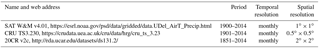
Several data sources are used in the study. The observed sub-daily SAT records and the associated metadata of Qingdao (1899–1913; Table 1) have been archived by DWD. Note that these SAT records from 1905 to 1914 have a high temporal resolution of 24 records for each day. The homogenized monthly SAT of Qingdao station (WMO station number is 54857) from 1961 to 2013 is selected from CMA, which has developed the first national homogenized temperature dataset (Li and Yan, 2009) and its updated version (Xu et al., 2013). Moreover, three gridded SAT datasets with high spatial resolution starting from the late 19th century have been used in the construction: (1) the monthly mean SAT from the global precipitation and temperature of Willmott and Matsuura, which is developed in the Department of Geography, University of Delaware (referred to as SAT W&M v4.01; Willmott and Matsuura, 2012); (2) the monthly mean SAT data of the Climatic Research Unit (Harris et al., 2013; referred as CRU TS3.230); and (3) the monthly mean SAT data of the 20th Century Reanalysis version 2c (referred to as 20CR v2c; Compo, et al., 2011). More details about the three datasets are shown in Table 2.
Table 1Coordinates, heights and daily observation times of Qingdao and Schatsykou in the earlier time.
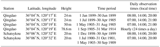
Table 2Three gridded SAT datasets that are used in this study.
2.2 Testing for significance of correlations and trends
When we test the significance of correlation between two time series and the significance of the presence of trends in a time series, an important question needs to be considered, that is, how large sample correlations and sample trends could be, even if the stochastic processes, which generate the series, are not correlated at all and exhibit no trends. Firstly, we have to make an assumption, namely the processes X and Y share no correlation, or segments of length L of the process have no trend. Standard procedures are available in the literature, namely p value for correlations and Mann–Kendall for trends (e.g., Kulkarni and von Storch, 1995; von Storch and Zwiers, 1999) that there are “no correlations” between the underlying processes and trends can hardly appear in limited segments of an infinite stationary time series.
In the case of correlations, the assumption is that the underlying processes are stationary (free of systematic trends) and serially independent, i.e., Xt and Xt+1 for any t are independent. In the case of trends, the assumption is the independence of . However, in geophysical cases, these assumptions are not satisfied – the result is that the null hypotheses are often falsely rejected (i.e., in cases where there are no correlations or no trends; cf. Kulkarni and von Storch, 1995) than stipulated by the significance level (normally 5 %).
A practical remedy for avoiding such errors is to deal with normalized series (mean = 0, standard deviation = 1) (and ) as follows:
- 1.
“detrend” the time series before testing for correlations between two time series Xt and Yt. Firstly, determining the linear fit and , and then do the hypothesis testing with and ,
- 2.
“prewhiten” the time series, by first determining the sample autocorrelation of the time series Xt of length L, and forming a series , and then testing for the null hypothesis of no trend.
The standard routines are applied to both cases. If the null hypothesis is rejected at the stipulated significance level of 5 %, then the sample trend , or the sample correlation , is “significant”.
In this paper, four seasonal mean SAT time series are defined by calculating the average of each three-month period: December(−1 yr)–January–February (Winter), March–April–May (Spring), June–July–August (Summer) and September–October–November (Autumn). Then, the linear trend of each season is also shown in this study; also the significance of each trend has been tested.
3.1 Processing of the earlier data from 1899 to 1913
3.1.1 Quality control and construction of missing data
The earlier SAT data from 1899 to 1913 have been digitized manually and passed through a quality check. The quality checking routine of DWD starts with a formal check, followed by climatological, temporal, repetition and consistency checks (Leiding et al., 2016). From April to December 1901, the original observations of Qingdao are not available. These missing values are filled in using the SAT time series of a neighboring station. We find that the value and variability in SAT monthly time series from July 1900 to December 1901 in Schatsykou exhibits a good agreement with these in Qingdao (Fig. 2). Consequently, the SAT data in Schatsykou is merged into the SAT data of Qingdao to fill the missing data.

Figure 2Comparison of the monthly mean SAT in Qingdao (solid line) with that in Schatsykou (dashed line) during July 1900 to December 1901.
Here, we have to point out that these quality checks above account for errors in coding and archiving, but are not efficient in dealing with inhomogeneities (Karl et al., 1993). In fact, changes in station height and changes in daily observational times (Table 1) can affect the SAT during 1899–1913. It is important in observational studies that the data used should be homogeneous (Trewin, 2010; J. F. Wang et al., 2014; Li et al., 2016). And in this study, homogenization of the data is the key factor. Thus, the homogenization of the SAT time series from 1899 to 1913 needs to be done in the next step.
3.1.2 Homogenization of SAT time series from 1899 to 1913
Inhomogeneities in land-based observations of air temperature may dampen or introduce noise to estimates of long-term air temperature trends. SAT data from 1961 to 2014 have been homogenized by CMA (Xu, et al., 2013). Here, we pay more attention to the detecting and adjusting of the SAT homogeneity from 1899 to 1913, which is newly digitized without homogenization.
Details of non-climatic factors were recorded in the metadata back to January 1899 (Table 1). Among these factors, the changes in observation height and daily observation times are the main causes of inhomogeneities. In the earlier time from January 1899 to April 1905, SAT was observed at 36∘04′ N, 120∘17′ E, which was a harbor near the coast of Qingdao (Fig. 2). From May 1905 to March 1914, SAT was observed at 36∘04′ N, 120∘19′ E, which was a small hill. The meteorology station was located at the top of this hill, without the effect of buildings and forest. Thus, the observation heights have been changed three times since 1899: 24 m (1 January 1899–30 April 1905), 50 m (1 May 1905–31 August 1905) and 78.6 m (1 September 1905–31 March 1914). The observing schedule was also changed in July 1899 from local time 08:00, 14:00, 20:00, to 07:00, 14:00, 21:00 (the same as Beijing time); and the observing schedule was changed again in April 1905 from local time 07:00, 14:00, 21:00 to hourly (24 times a day). In different periods the daily mean was calculated by the following different formulas:
In order to adjust the inhomogeneities caused by observation height change and observation times change, the best way is to find neighboring reference series and then modify the candidate series based on several mathematical methods. But actually it is hard and even impossible to find a reference series in such early times. In this case, air temperature in Qingdao was transformed into temperature at sea level using an average environmental lapse rate (6.0 ∘C km−1). Furthermore, to avoid the inconsistency of calculating a daily mean SAT from different observational times, the deviation caused by change of observational times is assessed firstly. We use Tdaily(I), Tdaily(II), Tdaily(III) to calculate the daily mean SAT using the observation data from 1908 to 1913, which were recorded 24 times a day. Then, monthly means in the whole period (1908–1913) are obtained by the average of the days in each month.
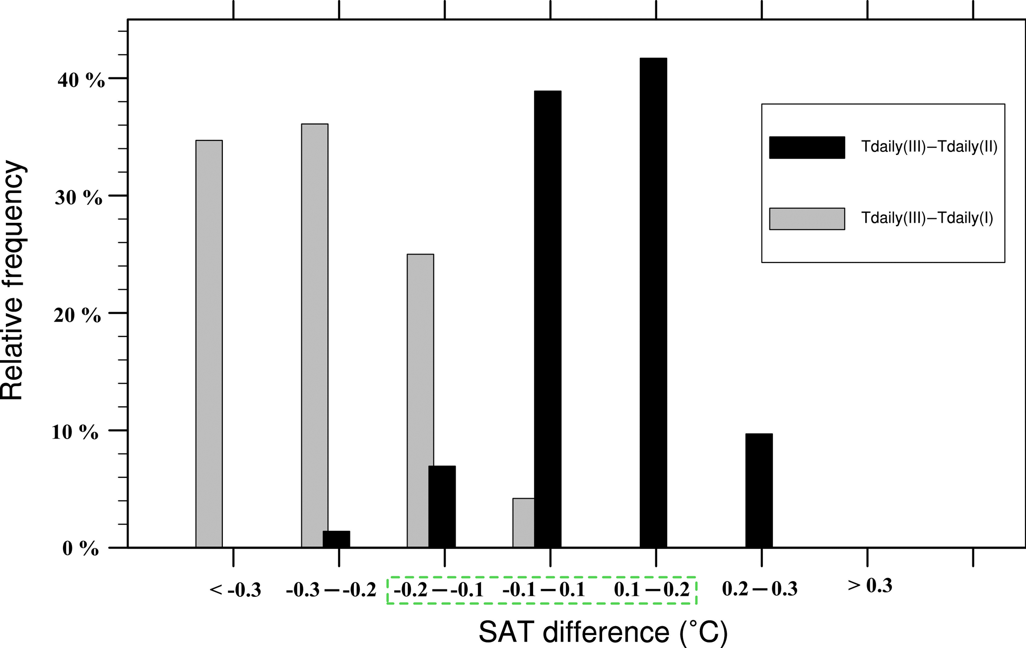
Figure 3Distribution of difference between the daily mean temperature Tdaily(III) and Tdaily(I) (gray bars) and difference between Tdaily(III) and Tdaily(II) (black bars) in the 72 months from January 1908 to December 1913 in Qingdao. The SAT differences in the green frame are considered as physically insignificant.
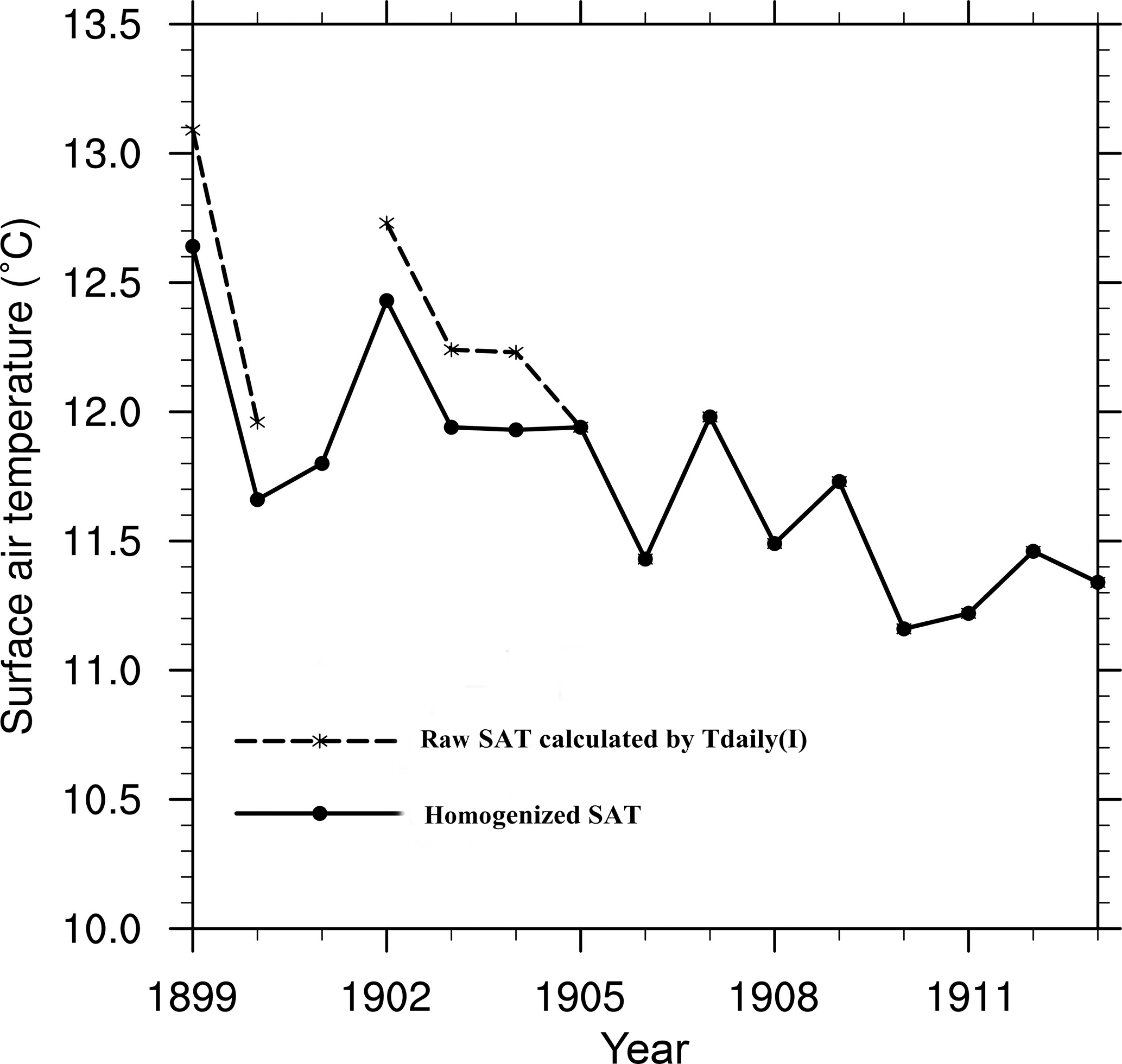
Figure 4Annual mean SAT series (∘C) of the raw and homogenized recorded at Qingdao from 1899 to 1913. Black line is the original observation series; red line is the homogenized series.
Generally, the SAT calculated by Tdaily(III) can represent the “real” daily mean SAT best. Thus, we calculate the frequency distributions of deviation between the monthly mean SAT of Tdaily(III) and Tdaily(II), as well as Tdaily(I) from January 1908 to December 1913 to assess the bias caused by different calculation formulas. Results are shown in Fig. 3. The majority of differences between Tdaily(III) and Tdaily(II) are from −0.1 to 0.2 ∘C. These discrepancies are small and can be ignored as physically insignificant. So the SAT from July 1899 to August 1905 do not need to be adjusted for the bias caused by Tdaily(II). However, the mean deviation between Tdaily(III) and Tdaily(I) is −0.27 ∘C and 35 % of the differences are larger than −0.3 ∘C. It suggests that the SAT calculated by Tdaily(I) has significant time-varying biases with that calculated by Tdaily(III), about 0.27 ∘C. Consequently, the SAT during January 1899 to June 1899 has applied to an adjustment of −0.27 ∘C. Figure 4 exhibits the annual mean SAT series before and after adjustment.
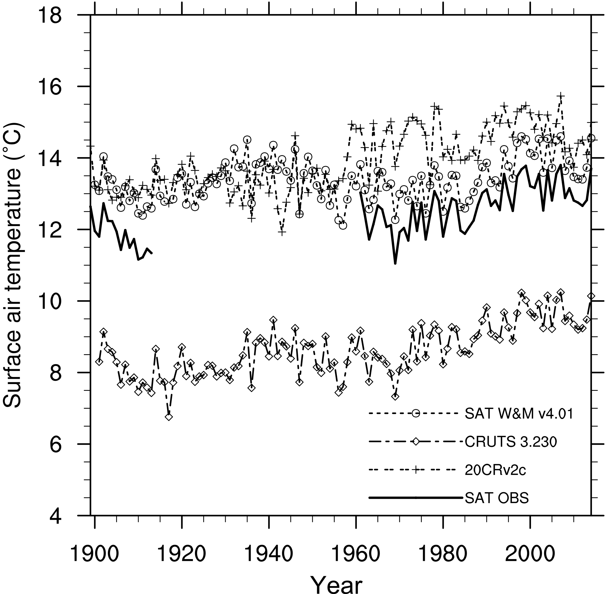
Figure 5Annual mean SAT time series in Qingdao from 1899 to 2013 (black solid line: SAT OBS; dashed line and cross: 20CR v2c; dashed line and circles: SAT W&M v4.01; dashed line and diamond: CRUTS 3.230).
3.2 Construction of SAT series in the past 115 years (1899–2014)
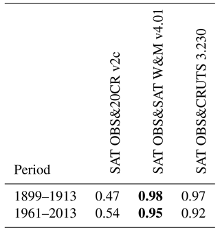
A previous study pointed out that the observation SAT from 1914 to 1960 was discontinuous with many missing data (Cao et al., 2013). For Qingdao station before 1960, the missing times of records were in July 1914 to March 1915, September 1937 to January 1938, and January 1951 to December 1960. However, all data from 1916 to 1950 has not been homogenized. In light of this, we attempt to use some grid-box datasets to fill with the gap from 1914 to 1959. Here, each of the three gridded SAT datasets have been evaluated for consistency with homogenized observations. Then the best one was used to estimate the SAT from 1914 to 1959. We calculated the correlation coefficient between the three SAT series with homogenized observations from DWD and CMA in Qingdao station (hereinafter referred to as SAT OBS) in two periods (1899–1913 and 1960–2014) after detrending described in Sect. 2.2. Results show that all of the correlation coefficients are statistically significant on the 95 % confidence interval (Table 3). The highest correlation coefficients (r = 0.98 and r = 0.95) are found between SAT OBS and SAT W&M v4.01. However, the correlation with the estimate of the CRUTS 3.230 shows rather low values, which are considerably smaller than those obtained with W&M v4.1 or 20CR v2c.
Table 3Correlation coefficients between the three SAT time series and the observational SAT time series in Qingdao. All of these time series have been detrended. The largest correlation coefficients are in bold.
Then, we compare the three annual mean SAT time series with the SAT OBS in Fig. 5. It can be seen that except for the 20CR v2c, the annual mean SAT series of W&M v4.01 and CRUTS 3.230 both have the similar climate variability with that of the SAT OBS. Interestingly, the difference between 20CR v2c and CRUTS 3.230 shows marked non-stationarities. In the first years, both series are similar, but exhibit relatively smaller interannual variability. Since about 1920 until 1950, the temperatures of 20CR v2c are mostly smaller than the CRUTS 3.320. But since about 1960 until 2005, the yearly means of 20CR v2c are strongly larger than CRUTS 3.320. The abrupt change in 20CR v2c around 1960 is not replicated in the W&M v4.01 series, and we suggest that this jump is an artifact in the analysis of 20CR v2c. Other non-stationarities have been found in the 20CR analyses (e.g., Krueger et al., 2014) and we suggest to rely more on the other two descriptions of past temperature variations. However, there is a relatively large systematic difference between the SAT OBS and the CRUTS 3.230 data and the difference even exceeds 3.5 ∘C (see also Cao et al., 2013). These discrepancies may derive from different quality control routines for data and the inconsistency of statistical methods used (Li et al., 2016). Based on these findings, we use SAT W&M v4.01 for filling the gap in the observational series between 1914 and 1959 to obtain continuous SAT series in Qingdao.
Using a linear regression method, each monthly mean SAT OBS in each period can be estimated from SAT W&M v4.01. Take SAT OBS in January for example, SAT OBS = (SAT W&M v4.01 + 0.62)∕0.95 during 1899–1913 and SAT OBS = (SAT W&M v4.01 + 1.15∕0.94) during 1960–2014. Then, we give the estimated linear relationship during 1914 to 1959 in January, SAT OBS = (SAT W&M v4.01 + 0.85)∕0.95 to get the monthly mean SAT OBS in the period of 1914–1959 in January. Consequently, monthly SAT OBS in each month from 1914 to 1959 was obtained. The SAT series in Qingdao from 1899 to 2014 is shown in Fig. 6.
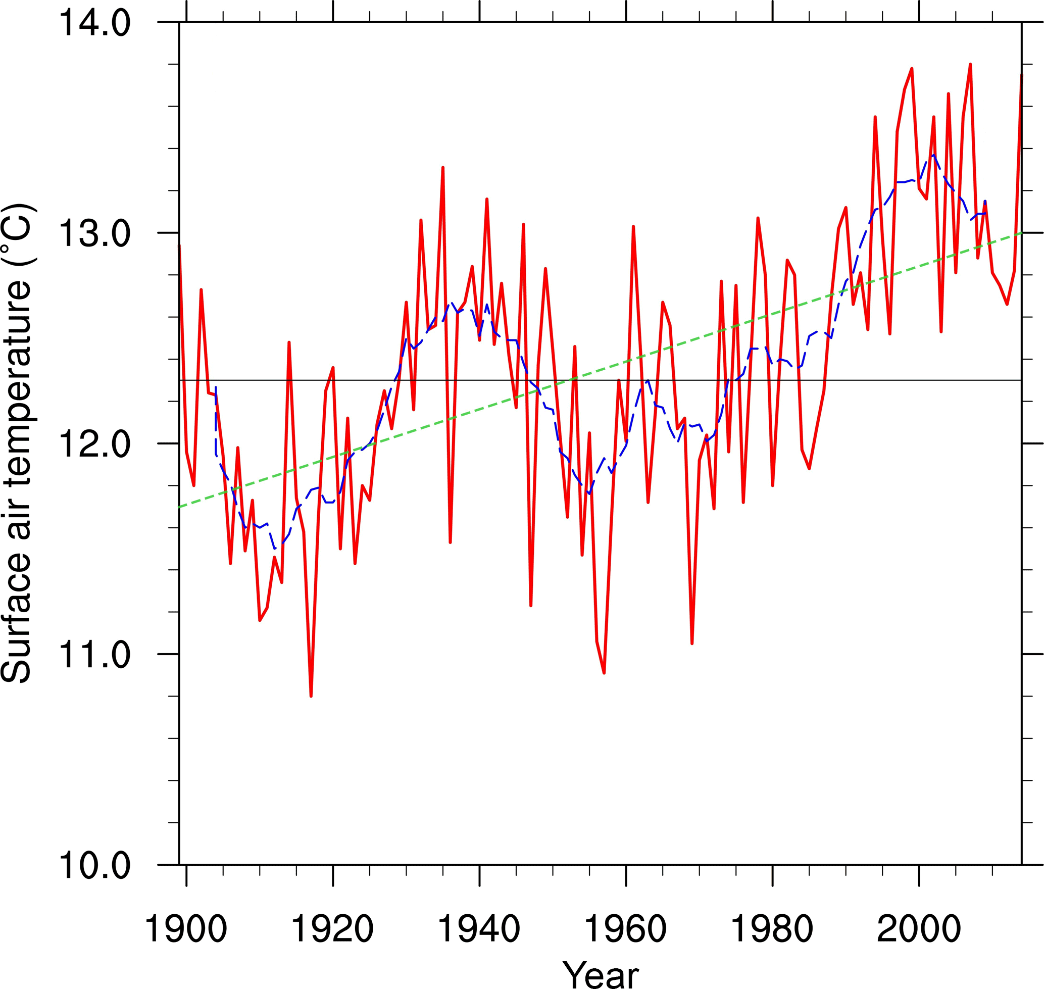
Figure 6Construction of annual mean SAT (∘C) in Qingdao for the period 1899–2014 (red solid line) and the 10-year running mean (long dashed line). The short dashed line represents the long-term linear trend. The thin black solid line shows the climate annual mean SAT relative to 1961–1990.
3.3 The temporal variations in the SAT trend of the constructed series
The newly constructed annual mean SAT in Qingdao from 1899 to 2014 (Fig. 6) exhibits a warming rate in Qingdao over the last 116 years of 0.11 ± 0.03 ∘C decade−1, slightly larger than the global mean warming rate over 1901–2012 (about 0.09 ∘C decade−1; IPCC AR5, 2013). It indicates that the warming trend is significant (significant at 95 % confidence intervals tested by the Mann–Kendall test, p value < 0.05). From the time series, we also find that the coldest years occurred in 1917 and 1969, with 11.03 and 11.05 ∘C. The warmest years occurred in 2007 and 1999, with annual means of 13.80 and 13.78 ∘C. Recently, Cao et al. (2013) calculated the average warming trend over the last hundred years based on SAT from 16 stations in China, with the rate of 0.15 ∘C decade−1, which is consistent with our result in Qingdao.
Since 2000, the SAT undergoes a decreasing trend, with a rate of −0.4 ∘C decade−1, even if the other SAT series (Fig. 5) exhibit positive SAT anomalies for the continuous 15 years (2000–2014). This slowdown or warming “hiatus” in this period is also found on regional and global scales. The Intergovernmental Panel on Climate Change Fifth Assessment Report (IPCC AR5) pointed out that during recent years (1998–2013), the global warming rate has slowed down. This period has been discussed in a number of papers (Kosaka and Xie, 2013; Smith, 2013) and has been known as a “hiatus” (Fyfe et al., 2013) or “global slowdown” (Guemas et al., 2013). Recent studies indicate that the recent “warming hiatus” is also found in Chinese SAT changes (J. F. Wang et al., 2014; Li et al., 2015). Proposed mechanisms for the recent warming hiatus at the global scale are still under debate, including changes in deep-ocean heat uptake, anthropogenic aerosols, solar variations, volcanoes and sea surface temperature (Meehl et al., 2011; Kaufmann et al., 2011; Kosaka and Xie, 2013). At regional and local scales, other factors may also play a significant role, which makes attribution challenging.
It is also interesting to note that during 1899–1910 there is another decreasing trend, with the rate of −1.1 ∘C decade−1, which is likely an expression of natural variability, as we have no noteworthy global or regional forcing during that time. This cooling rate is quite high, but the period extends only across 12 years, followed by a rapid warming for several decades until about 1940 (Fig. 6).
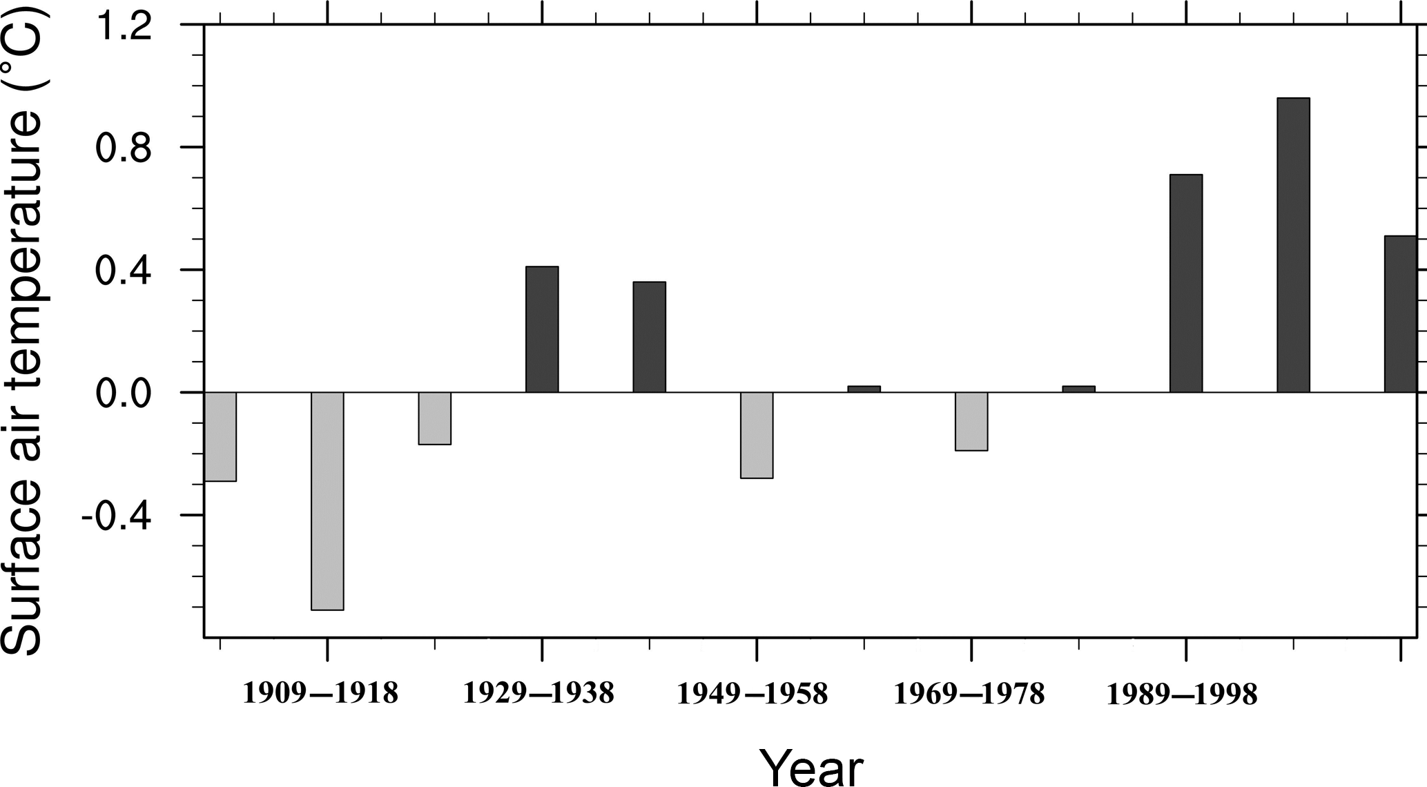
Figure 7Averaged annual mean SAT anomalies for each decade (∘C) in Qingdao during 1899–2014 relative to the 1961–1990 reference period (black line in Fig. 6; gray bar means negative values and black bar means positive values).
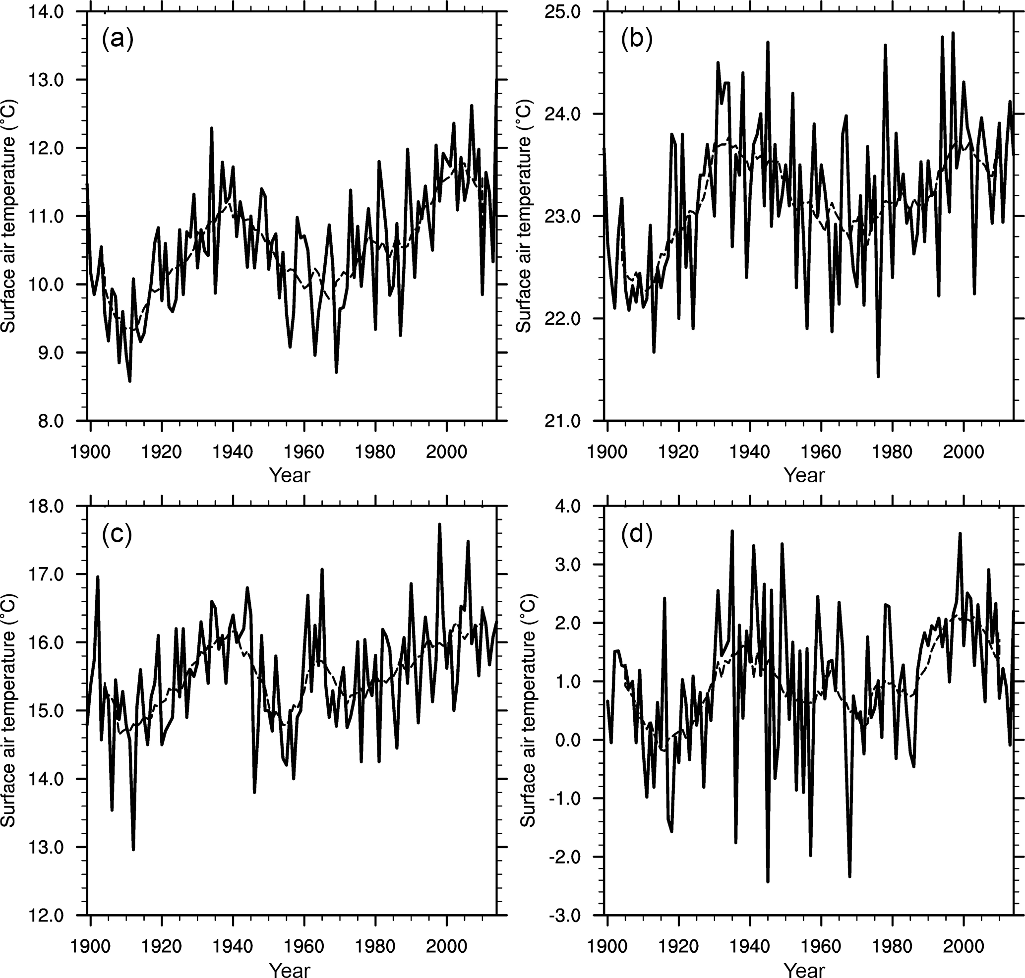
Figure 8Constructed seasonal mean SAT series (∘C) in Qingdao for the period 1899–2014 (solid line) and the 10-year running mean (dashed line). (a) Spring, (b) summer, (c) autumn and (d) winter.

Figure 9Differences in TX, TN and DTR between the period 1907–1913 and the period of 2007–2013 (∘C).
The constructed 10-year annual mean SAT from 1899 to 2014 are shown in Fig. 7. Five main periods are associated with larger than normal SAT. The three maximum warm periods occurred during 1989–1998, 1999–2008 and 2009–2014. The average anomaly SAT of 1999–2008 is the largest which is higher than normal of about 0.96 ∘C. On the other hand, cold periods occurred in the following decades: 1899–1908, 1909–1918 and 1949–1958.
The seasonal mean SAT time series are also shown in Fig. 8. The linear change trends and 95 % uncertainty ranges are also calculated, with the warming rate of about 0.12 ± 0.04 ∘C decade−1 in spring, 0.06 ± 0.04 ∘C decade−1 in summer, 0.08 ± 0.04 ∘C decade−1 in autumn and 0.10 ± 0.07 ∘C decade−1 in winter. These values suggest that the most significant warming occurred in spring, followed by winter. The interdecadal variations in the seasonal mean temperature in spring and winter appeared as a series of waves with a timescale of about 50–60 years. However, the trends in summer and autumn are much lower. The seasonal difference of the warming rate was also exhibited in other research on SAT in other stations of China, or SAT in the whole of China (Fong et al., 2009).
The homogenized monthly mean surface air temperature for Qingdao from 1899 to 2014 is provided and archived by the Deutscher Wetterdienst (DWD) web page under overseas stations of the Deutsche Seewarte (http://www.dwd.de/EN/ourservices/overseas_stations/ueberseedoku/doi_qingdao.html) in ASCII format. Users can also freely obtain a short description of the data at https://doi.org/10.5676/DWD/Qing_v1. And the data can be downloaded at http://dwd.de/EN/ourservices/overseas_stations/ueberseedoku/data_qingdao.txt.
Construction of a long-term homogeneous meteorological time series is essential for research in the field of climate change. Using quality control, interpolation and homogeneity methods, we objectively establish a set of homogenized monthly mean SAT series in Qingdao, China from 1899 to 2014. Three datasets were combined in this study, including the newly digitized observations of Qingdao station from the German National Meteorological Service from 1899 to 1913, adjusted SAT W&M v4.01 from Delaware University during 1914–1959 and homogenized SAT dataset from CMA during 1960–2014.
Based on the monthly SAT data, long-term changes in Qingdao, China are analyzed for the period 1899–2014. The main conclusions are as follows: (1) the SAT in Qingdao has a significant warming trend of 0.11 ± 0.04 ∘C decade−1 during 1899–2014. (2) There are two periods with cooling trends, they are 1899–1910 (−1.1 ∘C decade−1) and 2000–2013 (−0.4 ∘C decade−1). (3) There are seasonal differences in the warming rate with the largest warming rate in spring. These characteristics of the SAT variabilities in Qingdao agree well with the variabilities in SAT in the same region of China in the previous works.
Frankly, hourly observations in the early 20th century make it possible to compare the extreme temperature and diurnal cycle of temperature with present-day observations. Here we finally chose the period from 1 January 1907 to 31 December 1913 with little missing data. Then we compare the maximum temperature (TX), minimum temperature (TN) and diurnal temperature range (DTR; Table 4) in the period from 1 January 1907 to 31 December 1914 to those in the period from 1 January 2007 to 31 December 2013 (100-year interval). Hourly data from 1 January 2007 to 31 December 2014 are provided by CMA. Yearly mean daily TX (TN/DTR) temperature is defined by calculating the average of each daily TX (TN/DTR) temperature in a year. Then the differences in TX, TN and DTR between the two periods are shown in Fig. 9. In Fig. 9, the TX and TN are found to have significantly increased at the range of 1.2 to ∼ 2.7 ∘C and 1.0 to ∼ 2.4 ∘C. It means that relative to the years at the beginning of the 20th century, both of the TX and TN rise by ∼ 2.0 ∘C at the beginning of the 21st century. However, there is no notable increase or decrease in the DTR. Global annually averaged SAT has increased by 1.0 ∘C over the last 115 years (1901–2016) according to the Climate Science Special Report 2017 of USA. Compared to global warming, temperature warming in Qingdao is much stronger, which may be caused by the rapid industrialization in and around Qingdao. Based on such additional data, we can make further progress in our understanding of past, present and future climate change in the region.
From this study, we have also noticed that reconstruction and digitization of historical weather observations is important for extending time series or filling gaps and improving the gridded or reanalysis dataset. Furthermore, it is essential to be aware that metadata is important for homogenization of the time series, especially in the earlier times without reference series. We therefore agree with Allan et al. (2011, 2016) that longer and more spatially and temporally complete historical weather records could be recovered, imaged and digitized to expand the observational database. There is still a long way to go.
The authors declare that they have no conflict of interest.
This work was conducted by the lead author during a stay as visiting
scientist at the German Meteorological Service (Deutscher Wetterdienst, DWD)
and Federal Maritime and Hydrographic Agency (BSH) in Germany. We thank
Hamburg University's Cluster of Excellence CliSAP (Integrated Climate System
Analysis and Prediction) for funding the stay.
Edited by: David Carlson
Reviewed by: two anonymous referees
Allan, R., Brohan, P., Compo, G. P., Stone, R., Luterbacher, J., and Brönnimann, S.: The international atmospheric circulation reconstructions over the Earth (ACRE) initiative, B. Am. Meteorol. Soc., 1421–1425, https://doi.org/10.1175/2011BAMS3218.1, 2011.
Allan, R., Endfield, G., Damodaran, V., Adamson, G., Hannaford, M., Carroll, F., Macdonald, N., Groom, N., Jones, J., Williamson, F., Hendy, E., Holper, P., Arroyo-Mora, J. P., Hughes, L., Bickers, R., and Bliuc, A.-M.: Toward integrated historical climate research: the example of Atmospheric Circulation Reconstructions over the Earth, WIREs Clim. Change, 7, 164–174, https://doi.org/10.1002/wcc.379, 2016.
Cao, L., Zhao, P., Yan, Z., Jones, P., and Zhu, Y.: Instrumental temperature series in eastern and central China back to the nineteenth century, J. Geophys. Res.-Atmos., 118, 8197–8207, doi10.1002/jgrd.50615, 2013.
Compo, G. P., Whitaker, J. S., Sardeshmukh, P. D., Matsui, N., Allan, R. J., Yin, X., Gleason, B. E., Vose, R. S., Rutledge, G., Bessemoulin, P., Brönnimann, S., Brunet, M., Crouthamel, R. I., Grant, A. N., Groisman, P. Y., Jones, P. D., Kruk, M. C., Kruger, A. C., Marshall, G. J., Maugeri, M., Mok, H. Y., Nordli, Ø., Ross, T. F., Trigo, R. M., Wang, X. L., Woodruff, S. D., and Worley, S. J.: The twentieth century reanalysis project, Q. J. Roy. Meteor. Soc., 137, 1–28, https://doi.org/10.1002/qj.776, 2011.
Fong, S. K., Wu, C. S., Wang, A. Y., He, X. J., Wang, T., Leong, K. H., Lai, U., and Leong, B. Q.: Analysis of surface air temperature change in Macau during 1901–2007, Adv. Clim. Change Res., 5, 12–17, 2009 (in Chinese).
Fyfe, J. C., Gillett, N. P., and Zwiers, F. W.: Overestimated global warming over the past 20 years, Nat. Clim. Change, 3, 767–769, https://doi.org/10.1038/nclimate1972, 2013.
Guemas, V., Doblas-Reyes, F. J., Andrew-Burillo, I., and Asif, M.: Retrospective prediction of the global warming slowdown in the past decade, Nat. Clim. Change, 3, 649–653, https://doi.org/10.1038/nclimate1863, 2013.
Harris, I., Jones, P. D., Osborn, T. J., and Lister, D. H.: Updated high-resolution grids of monthly climatic observations – The CRU TS3.10 dataset, Int. J. Climatol., 34, 623–642, https://doi.org/10.1002/joc.3711, 2013.
Hasselmann, K.: On the signal-to-noise problem in atmospheric response studies, in: Meteorology over the tropical oceans, edited by: Shaw, B. D., Royal Meteorological Society, Bracknell, Berkshire, England, 251–259, 1979.
IPCC: Climate change 2013: The physical science basis. Contribution of working group I to the fifth assessment report of the intergovernmental panel on climate change. Cambridge University Press, Cambridge, United Kingdom and New York, NY, USA, 1535 pp., https://doi.org/10.1017/CBO9781107415324, 2013.
Karl, T. R., Jones, P. D., Knight, R. W., Kukla, G., and Plummer, N.: A new perspective on recent global warming: Asymmetric trends of daily maximum and minimum temperature, B. Am. Meteorol. Soc., 74, 1007–1023, https://doi.org/10.1175/1520-0477(1993)074<1007:ANPORG>2.0.CO;2, 1993.
Kaspar, F., Tinz, B., Mächel, H., and Gates, L.: Data rescue of national and international meteorological observations at Deutscher Wetterdienst, Adv. Sci. Res., 12, 57–61, https://doi.org/10.5194/asr-12-57-2015, 2015.
Kaufmann, R. K., Kauppi, H., Mann, M. L., and Stock, J. H.: Reconciling anthropogenic climate change with observed temperature 1998–2008, P. Natl. Acad. Sci. USA, 108, 11790–11793, 2011.
Kosaka, Y. and Xie, S. P.: Recent global warming hiatus tied to equatorial Pacific surface cooling, Nature, 501, 403–407, https://doi.org/10.1038/nature12534, 2013.
Krueger, O., Feser, F., Bärring, L., Kaas, E., Schmith, T., Tuomenvirta, H., and von Storch, H.: Comment on “Trends and low frequency variability of extra-tropical cyclone activity in the ensemble of Twentieth Century Reanalysis” by Xiaolan L. Wang, Y. Feng, G. P. Compo, V. R. Swail, F. W. Zwiers, R. J. Allan, and P. D. Sardeshmukh, Clim. Dynam., 2012, Clim. Dynam., 42, 1127–1128, https://doi.org/10.1007/s00382-013-1814-9, 2014.
Kulkarni, A. and von Storch, H.: Monte Carlo experiments on the effect of serial correlation on the Mann-Kendall-test of trends, Meteor. Z., 4, 82–85, 1995.
Leiding, T., Tinz, B., Gates, L., and Sedlatschek, R.: Standardized assessment of marine meteorological data from offshore platforms, Kurzfassungen der Meteorologentagung DACH Berlin, Deutschland, 14–18 März 2016, DACH2016-233, http://meetingorganizer.copernicus.org/DACH2016/DACH2016-233.pdf, 2016.
Li, Q. X. and Yan, W. Z.: Homogenized China daily mean/maximum/minimum temperature series 1960–2008, Atmospheric and Oceanic Science Letters, 2, 237–243, https://doi.org/10.1080/16742834.2009.11446802, 2009.
Li, Q. X., Su, Y., Xu, W. H., Wang, X. L., Jones, P., and Parker, D.: China experiencing the recent warming hiatus, Geophys. Res. Let., 42, 889–898, https://doi.org/10.1002/2014GL062773, 2015.
Li, Y., Mu, L., Wang, G. S., Fan, W. J., Liu, K. X., Li, H., and Zhang, Z. J.: The detecting and adjusting of the sea surface temperature data homogeneity over coastal zone of circum Bohai Sea, Haiyang Xuebao, 38, 27–39, https://doi.org/10.3969/j.issn.0253-4193.2016.03.003, 2016 (in Chinese).
Li, Q. X., Zhang, L., Xu, W. H., Zhou, T. J., Wang, J. F., Zhai, P. M., and Jones, P.: Comparisons of time series of annual mean surface air temperature for China since the 1900s: observations, model simulations, and extended reanalysis, B. Am. Meteorol. Soc., 98, 699–711, https://doi.org/10.1175/BAMS-D-16-0092.1, 2017.
Lin, X. C., Yu, S. Q., and Tang, G. L.: Series of average air temperature over China for the last 100-year period, Sci. Atmos. Sin., 19, 525–534, https://doi.org/10.3878/j.issn.1006-9895.1995.05.02, 1995 (in Chinese).
Meehl, G. A., Arblaster, J. M., Fasullo, J. T., Hu, A. and Trenberth, K. E.: Model-based evidence of deep-ocean heat uptake during surface-temperature hiatus periods, Nat. Clim. Change, 1, 360–364, https://doi.org/10.1038/nclimate1229, 2011.
Mitchell, T. D., Hulme, M., and New, M.: Climate data for political areas, Area, 34, 109–112, https://doi.org/10.1111/1475-4762.00062, 2002.
Qian, C., Yan, Z. W., Fu, C. B., and Tu, K.: Trends in temperature extremes in association with weather-intraseasonal fluctuation in eastern China, Adv. Atmos. Sci., 28, 284–296, https://doi.org/10.1007/s00376-010-9242-9, 2011.
Qian, W. H. and Zhu, Y. F.: Climate change in China from 1880-1998 and its impact on the environmental condition, Clim. Change, 50, 419–444, https://doi.org/10.1023/A:1010673212131, 2001.
Smith, D.: Oceanography: has global warming stalled?, Nat. Clim. Change, 3, 618–619, https://doi.org/10.1038/nclimate1938, 2013.
Soon, W., Dutta, K., Legates, D. R., Velasco, V., and Zhang, W. J.: Variation in surface air temperature of China during the 20th century, J. Atmos. Sol.-Terr. Phy., 73, 2331–2344, https://doi.org/10.1016/j.jastp.2011.07.007, 2011.
Tang, G. L. and Ren, G. Y.: Reanalysis of surface air temperature change of the last 100 years over China, Clim. Environ. Res., 10, 791–798, https://doi.org/10.3878/j.issn.1006-9585.2005.04.10, 2005 (in Chinese).
Tang, G. L., Ding, Y. H., Wang, S.W., Ren, G. Y., Liu, H. B., and Zhang, L.: Comparative analysis of the time series of the time series of surface air temperature over China for the last 100 years, Adv. Clim. Change Res., 5, 71–78, 2009 (in Chinese).
Trewin, B.: Exposure, instrumentation, and observing practice effects on land temperature measurements, WIREs Clim. Change, 1, 490–506, https://doi.org/10.1002/wcc.46, 2010.
U.S. Global Change Research Program (USGCRP): Climate Science Special Report: Fourth National Climate Assessment, Volume I. Washington, DC, USA, 470 pp., https://doi.org/10.7930/J0J964J6, 2017.
von Storch, H. and Zwiers, F. W.: Statistical Analysis in Climate Research, Cambridge University Press, London, 1999.
Wang, J., Xu, C., Hu, M., Li, Q., Yan, Z., Zhao, P., and Jones, P.: A new estimate of the China temperature anomaly series and uncertainty assessment in 1900–2006, J. Geophy. Res.-Atmos., 119, 1–9, 2014.
Wang, S. W. and Gong, D.: Enhancement of the warming trend in China, Geophys. Res. Let., 27, 2581–2584, https://doi.org/10.1029/1999GL010825, 2000.
Wang, S. W., Zhu, J. H., and Cai, J. N.: Interdecadal variability of Temperature and precipitation in China since 1880, Adv. Atmos. Sci., 21, 307–313, https://doi.org/10.1007/BF02915560, 2004.
Wang, J., Xu, C., Hu, M., Li, Q., Yan, Z., Zhao, P., and Jones, P.: A new estimate of the China temperature anomaly series and uncertainty assessment in 1900–2006, J. Geophy. Res.-Atmos., 119, 1–9, https://doi.org/10.1002/2013JD020542, 2014.
Willmott, C. J. and Matsuura, K.: Terrestrial air temperature: 1900–2010 gridded monthly time series (V3.01), http://climate.geog.udel.edu/~climate/html_pages/Global2011/README.GlobalTsT2011.html (last access: March 2018), 2012.
Xu, W. H, Li, Q. X., Wang, X. L., Yang, S., Cao, L. J., and Feng, Y.: Homogenization of Chinese daily surface air temperature and analysis of trends in the extreme temperature indices, J. Geophys. Res.-Atmos., 118, 9708–9720, https://doi.org/10.1002/jgrd.50791, 2013.
Zorita, E., Stocker, T., and von Storch, H.: How unusual is the recent series of warm years?, Geophys. Res. Lett. 35, L24706, https://doi.org/10.1029/2008GL036228, 2008.