the Creative Commons Attribution 4.0 License.
the Creative Commons Attribution 4.0 License.
 | 06 Jun 2018
History of chemically and radiatively important atmospheric gases from the Advanced Global Atmospheric Gases Experiment (AGAGE)
Ronald G. Prinn
Ray F. Weiss
Jgor Arduini
Tim Arnold
H. Langley DeWitt
Paul J. Fraser
Anita L. Ganesan
Jimmy Gasore
Christina M. Harth
Ove Hermansen
Jooil Kim
Paul B. Krummel
Shanlan Li
Zoë M. Loh
Chris R. Lunder
Michela Maione
Alistair J. Manning
Ben R. Miller
Blagoj Mitrevski
Jens Mühle
Simon O'Doherty
Sunyoung Park
Stefan Reimann
Matt Rigby
Takuya Saito
Peter K. Salameh
Roland Schmidt
Peter G. Simmonds
L. Paul Steele
Martin K. Vollmer
Ray H. Wang
Bo Yao
Yoko Yokouchi
Dickon Young
Lingxi Zhou
We present the organization, instrumentation, datasets, data interpretation, modeling, and accomplishments of the multinational global atmospheric measurement program AGAGE (Advanced Global Atmospheric Gases Experiment). AGAGE is distinguished by its capability to measure globally, at high frequency, and at multiple sites all the important species in the Montreal Protocol and all the important non-carbon-dioxide (non-CO2) gases assessed by the Intergovernmental Panel on Climate Change (CO2 is also measured at several sites). The scientific objectives of AGAGE are important in furthering our understanding of global chemical and climatic phenomena. They are the following: (1) to accurately measure the temporal and spatial distributions of anthropogenic gases that contribute the majority of reactive halogen to the stratosphere and/or are strong infrared absorbers (chlorocarbons, chlorofluorocarbons – CFCs, bromocarbons, hydrochlorofluorocarbons – HCFCs, hydrofluorocarbons – HFCs and polyfluorinated compounds (perfluorocarbons – PFCs), nitrogen trifluoride – NF3, sulfuryl fluoride – SO2F2, and sulfur hexafluoride – SF6) and use these measurements to determine the global rates of their emission and/or destruction (i.e., lifetimes); (2) to accurately measure the global distributions and temporal behaviors and determine the sources and sinks of non-CO2 biogenic–anthropogenic gases important to climate change and/or ozone depletion (methane – CH4, nitrous oxide – N2O, carbon monoxide – CO, molecular hydrogen – H2, methyl chloride – CH3Cl, and methyl bromide – CH3Br); (3) to identify new long-lived greenhouse and ozone-depleting gases (e.g., SO2F2, NF3, heavy PFCs (C4F10, C5F12, C6F14, C7F16, and C8F18) and hydrofluoroolefins (HFOs; e.g., CH2 = CFCF3) have been identified in AGAGE), initiate the real-time monitoring of these new gases, and reconstruct their past histories from AGAGE, air archive, and firn air measurements; (4) to determine the average concentrations and trends of tropospheric hydroxyl radicals (OH) from the rates of destruction of atmospheric trichloroethane (CH3CCl3), HFCs, and HCFCs and estimates of their emissions; (5) to determine from atmospheric observations and estimates of their destruction rates the magnitudes and distributions by region of surface sources and sinks of all measured gases; (6) to provide accurate data on the global accumulation of many of these trace gases that are used to test the synoptic-, regional-, and global-scale circulations predicted by three-dimensional models; and (7) to provide global and regional measurements of methane, carbon monoxide, and molecular hydrogen and estimates of hydroxyl levels to test primary atmospheric oxidation pathways at midlatitudes and the tropics. Network Information and Data Repository: http://agage.mit.edu/data or http://cdiac.ess-dive.lbl.gov/ndps/alegage.html (https://doi.org/10.3334/CDIAC/atg.db1001).
Please read the corrigendum first before continuing.
-
Notice on corrigendum
The requested paper has a corresponding corrigendum published. Please read the corrigendum first before downloading the article.
-
Article
(4605 KB)
-
The requested paper has a corresponding corrigendum published. Please read the corrigendum first before downloading the article.
- Article
(4605 KB) - Corrigendum
- BibTeX
- EndNote


The Advanced Global Atmospheric Gases Experiment (AGAGE: 1993–present) and its predecessors (Atmospheric Lifetime Experiment, ALE: 1978–1981; Global Atmospheric Gases Experiment, GAGE: 1982–1992) have measured the greenhouse gas and ozone-depleting gas composition of the global atmosphere continuously since 1978. The ALE program was instigated to measure the then five major ozone-depleting gases (CFC-11 (CFCl3), CFC-12 (CCl2F2), CCl4, CH3CCl3, N2O) in the atmosphere four times per day using automated gas chromatographs with electron-capture detectors (GC-ECDs) at four stations around the globe and to determine the atmospheric lifetimes of the purely anthropogenic of these gases from their measurements and industry data on their emissions (Prinn et al., 1983a). The GAGE project broadened the global coverage to five stations, the number of gases being measured to eight (adding CFC-113 (CCl2FCClF2), CHCl3, and CH4 to the ALE list), and the frequency to 12 per day by improving the GC-ECDs and adding gas chromatographs with flame-ionization detectors (GC-FIDs; Prinn et al., 2000). The AGAGE program then significantly improved upon the GAGE instruments by increasing their measurement precision and frequency (to 36 per day) and adding gas chromatographs with mercuric oxide reduction detectors, to measure 10 biogenic and/or anthropogenic gases overall (adding H2 and CO to the GAGE list). AGAGE also introduced powerful new gas chromatographs with mass spectrometric detection and cryogenic pre-concentration measuring over 50 trace gases 20 times per day. In this overview paper, while we address the entire 1978–present database and its public availability, we focus more on the evolution of the network after 2000; details of the period before that are addressed in the previous comprehensive overviews provided by Prinn et al. (2000) and Prinn et al. (1983a). The case for high-frequency measurement networks like AGAGE with data available to operators in real time is strong, and the observations and their interpretation are important inputs to the scientific understanding of ozone depletion and climate change. AGAGE is characterized by its capability to measure globally the trends at high frequency and estimate emissions from these trends for all of the important species in the Montreal Protocol on Substances that Deplete the Ozone Layer, and all of the important non-carbon-dioxide (non-CO2) trace gases assessed by the Intergovernmental Panel on Climate Change. More recently, AGAGE has also been measuring CO2 using high-frequency optical spectroscopy (focusing on sites where such measurements are not made by other groups; Sect. 2.3 and 2.4). The scientific objectives of AGAGE (summarized in the Abstract) are of considerable significance in furthering our understanding of important global chemical and climatic phenomena. The remainder of this Introduction is devoted to describing the network of stations (Sect. 1.1), the measurements (Sect. 1.2), and the place of AGAGE in the global observing system (Sect. 1.3). Then Sect. 2 addresses the instrumentation, calibration, and station infrastructure, Sect. 3 the data analysis and modeling, Sect. 4 the scientific accomplishments, and Sect. 5 the AGAGE data availability.
1.1 A Global network of stations
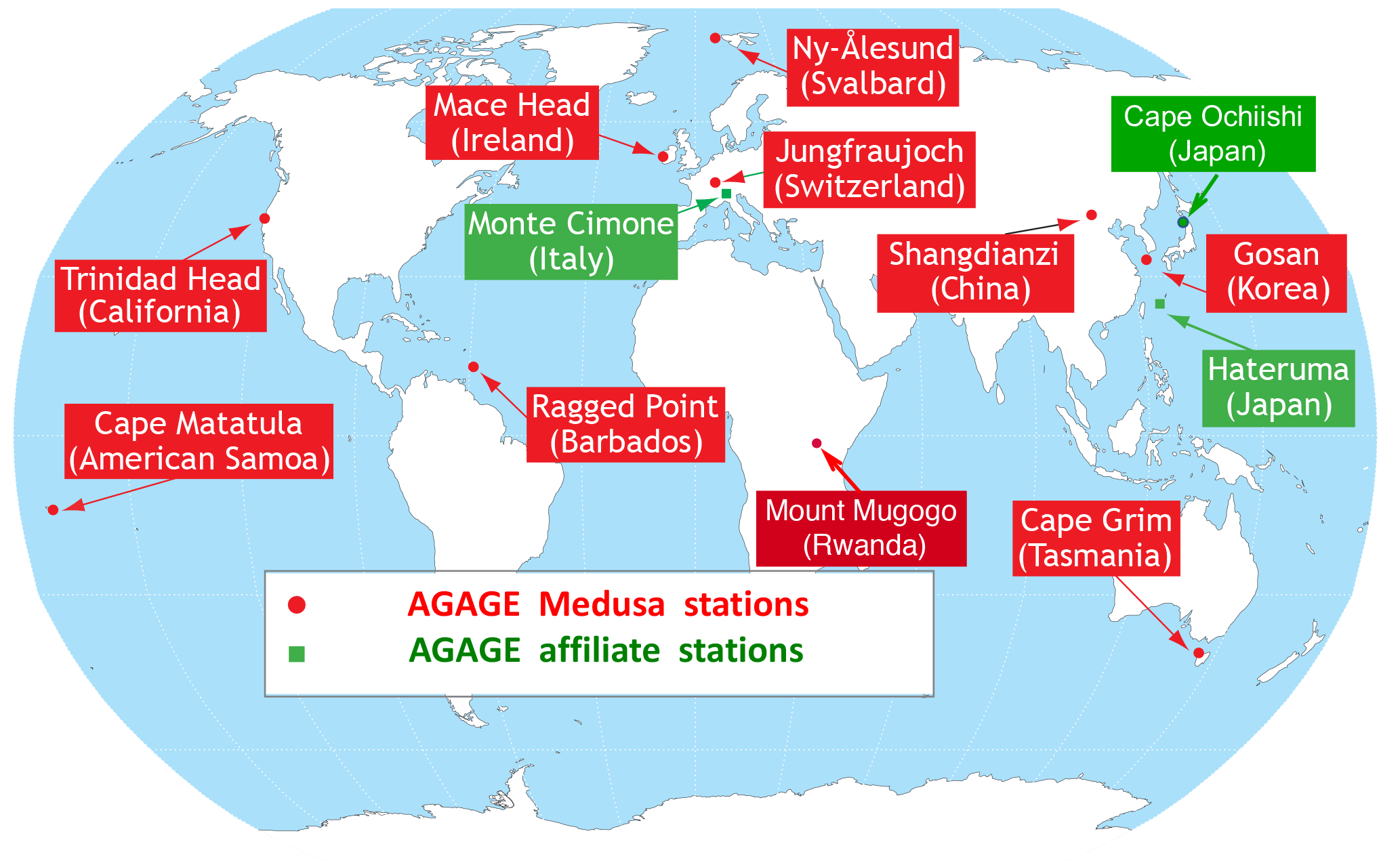
Figure 1Locations of the 10 current AGAGE primary stations (red highlighted stations) that have Medusa gas chromatograph–mass spectrometer (GC-MS) instruments and the 3 current AGAGE affiliate stations (green highlighted stations) that have alternative pre-concentration GC-MS instruments. AGAGE and the other major global air sampling network, NOAA-ESRL-GMD, are independent but closely cooperating, including frequent data intercomparisons, especially at the American Samoa shared site.
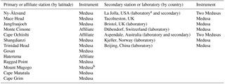
The ALE/GAGE/AGAGE stations are coastal or mountain sites around the world, chosen primarily to provide accurate measurements of trace gases whose lifetimes are long compared to global atmospheric circulation times (Fig. 1). The 10 “primary” AGAGE stations that all share common calibrations and gas chromatographic–mass spectrometric instrumentation (see Sect. 1.2) are the following: (a) on Ireland's west coast, first at Adrigole (52∘ N, 10∘ W; 50 m (inlet height a.s.l. here and for all other stations), 1978–1983), then at Mace Head (53∘ N, 10∘ W; 25 m 1987 to present); (b) on the US west coast, first at Cape Meares, Oregon (45∘ N, 124∘ W; 30 m, 1979–1989), then at Trinidad Head, California (41∘ N, 124∘ W; 140 m, 1995 to present); (c) at Ragged Point, Barbados (13∘ N, 59∘ W; 42 m, 1978 to present); (d) at Cape Matatula, American Samoa (14∘ S, 171∘ W; 77 m, 1978 to present); (e) at Cape Grim, Tasmania, Australia (41∘ S, 145∘ E; 164 m, 169 m, 1978 to present); (f) on the Jungfraujoch, Switzerland (47∘ N, 8∘ E; 3580 m, 2000 to present); (g) on Zeppelin Mountain, Ny-Ålesund, Svalbard, Norway (79∘ N, 12∘ E; 489 m, 2001 to present); (h) at Gosan, Jeju Island, Korea (33∘ N, 126∘ E; 89 m, 2007 to present); (i) at Shangdianzi, China (41∘ N, 117∘ E; 383 m, 2010 to present with gap) and (j) Mt. Mugogo, Rwanda (1.6∘ S, 29.6∘ E; 2640 m, 2015 to present). The AGAGE network also includes three AGAGE-compatible (but not identical) instruments in the following locations: (k) Hateruma Island, Japan (24∘ N, 123.8∘ E; 47 m, 2004 to present); (l) Cape Ochiishi, Japan (43∘ N, 145.5∘ E; 100 m, 2006 to present), and (m) Monte Cimone, Italy (44∘ N, 10∘ E; 2165 m, 2004 to present). These are called AGAGE “affiliate” stations in Fig. 1. There are also “secondary”, usually continental and some urban, stations that are linked to and complement the primary and affiliate stations (discussed below).
1.2 Measurements
At its primary stations, AGAGE uses in situ gas chromatography with mass spectrometry (GC-MS) in the “Medusa” system (Miller et al., 2008; Arnold et al., 2012) to measure over 50 largely synthetic gases including hydrochlorofluorocarbons (e.g., HCFC-22; CHClF2) and hydrofluorocarbons (e.g., HFC-134a; CH2FCF3), which are interim or long-term alternatives to chlorofluorocarbons (CFCs) now restricted by the Montreal Protocol, other hydrohalocarbons (e.g., methyl chloride; CH3Cl), halons (e.g., Halon-1211; CBrClF2), perfluorocarbons (e.g., PFC-14; CF4), and trace chlorofluorocarbons, all of which, except CH3Cl, are involved in the Montreal or Kyoto Protocol. Affiliate stations use similar but not identical cryogenic pre-concentration GC-MS systems (Maione et al., 2013; Yokouchi et al., 2006).
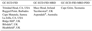
At its Mace Head, Trinidad Head, Ragged Point, Cape Matatula, and Cape Grim primary stations, AGAGE also uses in situ gas chromatographs (GC) with electron-capture detection (ECD), flame-ionization detection (FID), mercuric oxide reduction detection (MRD, at Mace Head and Cape Grim only), and pulsed discharge detection (PDD, at Cape Grim only) to measure five biogenic–anthropogenic gases (methane – CH4, nitrous oxide – N2O, and chloroform – CHCl3 at all sites; carbon monoxide – CO and hydrogen – H2 at Mace Head and Cape Grim only) and five anthropogenic gases at all five sites: CFC-11 (CCl3F), CFC-12 (CCl2F2), and CFC-113 (CCl2FCClF2), methyl chloroform (CH3CCl3), and carbon tetrachloride (CCl4) 36 times per day (Prinn et al., 2000). The list of gases measured with these gas chromatography “multidetector” (GC-MD) systems includes the three major chlorofluorocarbons (CFCs) restricted by the Montreal Protocol and the four major long-lived non-CO2 greenhouse gases (GHGs). Table 1 lists all the major gases being measured in AGAGE using the Medusa GC-MS and GC-MD instruments, their 2016 global average mole fractions, and their typical measurement precisions.
Table 1Primary AGAGE measured species using Medusa GC-MS and GC-MD systems. Gases measured with Medusa GC-MS and GC-MD only are in black regular font; those measured with both systems are in italic font. Calibrations are on AGAGE SIO gravimetric scales (Sect. 2.6) unless otherwise noted.
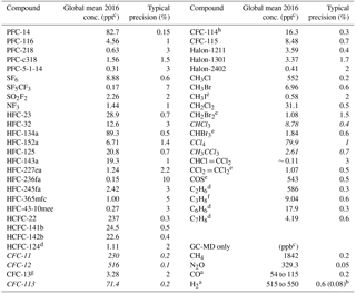
a CO and H2 measured at Mace Head and Cape Grim only (range for annual means of these two stations given). b GC-PDD system at Cape Grim. c ppt: parts per trillion and ppb: parts per billion. d Preliminary (AGAGE) scale (Sect. 2.6), e preliminary (transfer of NOAA) scale (Sect. 2.6), f preliminary (Empa) scale (Sect. 2.6), g METAS-2017 (Empa) scale (Sect. 2.6), h quasi-linear sum of CFC-114 and CFC-114a.
The precisions for each species are determined from the interspersed measurements of the on-site station calibration tanks and are reported along with the mole fractions of the interspersed atmospheric measurements in the AGAGE data archives. In general the precisions in Table 1 are highest (< 0.1 %) for the species with the highest absolute mole fractions and lowest (∼ 10 %) for those with the lowest mole fractions; there are also more subtle differences depending on the species behavior in the trapping (Medusa), separation (GC), and detection (MS, MD; ECD, FID, MRD) stages. The accuracy of the measurements is determined by calibration scale and tertiary tank accuracies that are discussed in Sect. 2.6.
Recent developments have enabled precise analyses of CH4, CO2, CO, and N2O by laser spectroscopic detection to begin in AGAGE. These optical instruments are now expanding the measurement capabilities within AGAGE, and there are advantages in switching from the GC-MD approach for measuring CH4, N2O, and CO to these less operationally demanding optical spectroscopy methods resulting in near-continuous measurements of comparable or better precision. As discussed in Sect. 2.3 and 2.4, this transition is happening already at several AGAGE stations. The GC-MD and optical spectroscopy instruments will follow the AGAGE protocol used for all cases in which a new improved instrument replaces an earlier one; namely, the two instruments are run together for at least several months (and years for gases currently measured on both the GC-MD and Medusa GC-MS) to ensure data comparability and verify improvements.
Each instrument system is automated and under computer control. All chromatograms, instrumental data, and operator logs are transmitted via the internet to the data processing sites. AGAGE includes timely public archiving and publication of all data, regular intercomparisons of AGAGE measurements, absolute calibrations with other networks (e.g., NOAA's Global Monitoring Division, GMD), and contributions to national and international assessments of ozone depletion and climate change. The data are calibrated against on-site air standards, which are calibrated relative to off-site parent standards before and after use at each station. AGAGE depends upon well-defined absolute gravimetric calibration procedures that are repeated periodically to ensure the accuracy of the long-term measured trends (Prinn et al., 2000).
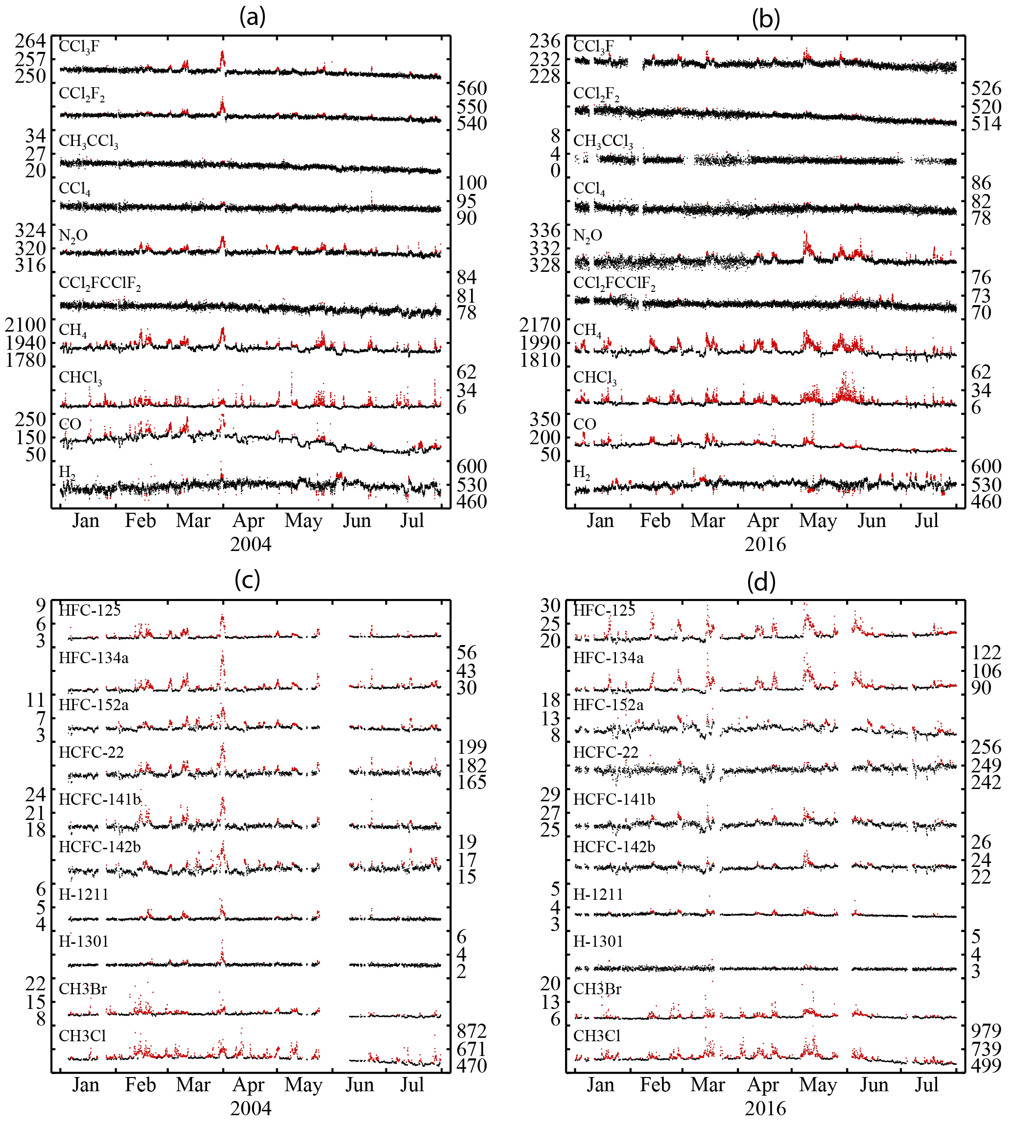
Figure 2A total of 7 months of data for gases measured at Mace Head, Ireland: (1) with the GC-MD in (a) 2004 and (b) 2016 (units: mole fractions; ppb for N2O, CH4, H2, and CO; ppt for all others) and (2) with the Medusa GC-MS for selected gases in (c) 2004 and (d) 2016 (units: mole fractions in ppt for all gases). In all four panels, measurements in polluted air originating from Europe (also in air affected by local sinks; see text) are shown in red, while those in clean air off the Atlantic Ocean are shown in black. Note that pollution events are defined separately for each gas due to their often differing sources.
To emphasize the need for very frequent real-time measurements we show data for several trace gases (Fig. 2a–d) for the years 2004 and 2016. These GC-MD and GC-MS data demonstrate the existence of regional pollution-induced or local sink-induced (e.g., for H2; shown in red) and large-scale transport-induced (shown in black) variability, which are not captured with weekly flask measurements typically designed to avoid local pollution. Our approach for identifying these pollution events is discussed in Sect. 3.1. Note also the evolution of the sizes of these pollution events between 2004 and 2016 associated with the decreases in the emissions of regulated gases and the growth of emissions of unregulated ones. This high-frequency sampling enables the pollution events in particular to be used to estimate emissions from nearby source regions (e.g., Cape Grim station for SE Australian emissions; e.g., Dunse et al., 2005; Stohl et al., 2009; O'Doherty et al., 2009; Fraser et al., 2014; Lunt et al., 2015), Trinidad Head for the west coast US emissions (e.g., Li et al., 2005; O'Doherty et al., 2009; Lunt et al., 2015; Fortems-Cheiney et al., 2015), Mace Head and the other European stations for European and in some cases eastern USA emissions (e.g., O'Doherty et al., 2009; Stohl et al., 2009; Keller et al., 2012; Simmonds et al., 2015; Lunt et al., 2015; Fortems-Cheiney et al., 2015; Graziosi et al., 2017), and Hateruma, Shangdianzi, and Gosan for East Asian emissions (e.g., Stohl et al., 2009, 2010; Kim et al., 2010; Li et al., 2011; Yao et al., 2012a, b; Saito et al., 2015; Fang et al., 2015; Lunt et al., 2015; Fortems-Cheiney et al., 2015). The sources of many anthropogenic and natural trace gases measured in AGAGE are often colocated so that measurement of a wide range of gases enhances the ability to accurately estimate their sources and sinks. The AGAGE data in graphical and digital forms are available for most stations at the AGAGE website: http://agage.mit.edu (last access: 21 May 2018) (Sect. 3.2).
1.3 Integral element of the global observing system
AGAGE is part of a powerful complementary observing system that is measuring various aspects of the evolving composition of Earth's atmosphere and providing the fundamental understanding needed to preserve this vital sphere of life on our planet. Sharing the AGAGE surface-based perspective are, for example, the remote-sensing Network for Detection of Atmospheric Composition Change (NDACC; see De Mazière et al., 2018) supported by NASA and other agencies and nations (AGAGE is an NDACC Cooperating Network) and the NOAA-ESRL Global Monitoring Division in situ and flask networks. AGAGE contributes to the World Meteorological Organization's Global Atmosphere Watch (WMO-GAW) and regularly provides its data to the WMO-GAW's World Data Center for Greenhouse Gases (WDCGG) website (see Sect. 5). AGAGE European stations provide data to the Integrated Carbon Observation System (ICOS)that coordinates pan-European observations of GHGs, and Monte Cimone, Jungfraujoch, and Ny Ålesund are now formally joining. Also measuring atmospheric composition (as column profiles or abundances) are instruments onboard the NASA TERRA and AURA satellites and the ESA ENVISAT satellite. Aircraft- and balloon-borne instruments provide vital in situ measurements in the middle troposphere and lower stratosphere. The combination of all of these complementary data with state-of-the-art global chemistry and circulation models is providing major advances in our understanding of the global sources, chemistry, transport, and sinks of atmospheric trace substances and allows for the determination of atmospheric composition and air quality, the radiative forcing of climate change, and impacts on stratospheric ozone.
The AGAGE program has placed a strong emphasis on instrumental innovation and the gravimetric preparation of primary standards to obtain high-frequency and high-precision automated trace gas measurements at all the AGAGE measurement sites. In this section, the first four subsections discuss the AGAGE GC-MD (Sect. 2.1), Medusa GC-MS (Sect. 2.2), optical spectroscopy (Sect. 2.3), and isotopic (Sect. 2.4) instruments. Then we address data acquisition and processing (Sect. 2.5), instrumental calibration (Sect. 2.6), primary and affiliate station facilities and infrastructure (Sect. 2.7), secondary stations (Sect. 2.8), and stored air archives (Sect. 2.9).
Table 2GC–multidetector instruments at current AGAGE primary and secondary stations. Detectors: ECD for CFC-11, CFC-12, CFC-113, CH3CCl3, CCl4, N2O, and CHCl3; FID for CH4; MRD for CO and H2; and PDD for H2.
a Modified version of the GC-MD without FID channel. b Uses three individual GC systems with ECD, FID, and MRD detectors.
In the early 1990s the GC-MD instruments were developed and deployed at the Mace Head, Trinidad Head, Ragged Point, Cape Matatula, and Cape Grim stations and at the Scripps Institution of Oceanography (SIO) calibration laboratory (Prinn et al., 2000). In the late 1990s, AGAGE pioneered the deployment of automated GC-MS instruments at our stations in Mace Head and Cape Grim and at the University of Bristol. These instruments featured an adsorption–desorption system (ADS) with cryogenic (−50 ∘C) pre-concentration of analytes from 2 L air samples (Simmonds et al., 1995). The technological developments incorporated into these instruments, the methods of data collection, transmission, and processing, the primary and secondary calibration standards produced at the SIO calibration laboratory, and the on-site tertiary (from SIO) and quaternary (calibrated on-site from the tertiary) standards necessary to sustain the AGAGE network are partly described in the first AGAGE overview (Prinn et al., 2000), but updated here in Sect. 2.6 and 2.7.
Beginning in the early 2000s, the AGAGE team recognized that modern refrigeration technology made it possible to make major improvements to the ADS concept and to greatly extend the range of compounds that could be measured by enhanced cryogenic pre-concentration at −165 ∘C. As a result, the AGAGE GC-MS effort was redirected to the development of the new Medusa instrument (Miller et al., 2008; Arnold et al., 2012).
2.1 GC–multidetector instruments
The current AGAGE GC-MD instruments replaced the earlier GAGE GC-MD instruments in 1993–1996 (Table 2). These Agilent© GC instruments employ two electron-capture detector (ECD) channels and one flame-ionization detection (FID) channel to measure the principal chlorine-bearing anthropogenic ozone-depleting compounds now banned by the Montreal Protocol (CFC-11, CFC-12, CFC-113, CCl4, and CH3CCl3), as well as the both natural and anthropogenic compounds N2O, CH4, and CHCl3 (see Table 1). The GC-MDs at Mace Head and Cape Grim include an extra channel for the measurement of CO and H2 by a mercuric oxide reduction detector (MRD; Prinn et al., 2000). In early 2015, the GC-MD system at Cape Grim also added a further extra channel for the measurement of H2 by pulsed discharge detector (PDD), bringing a more than 10-fold improvement in precision. The GC-MD measurements are made on dried whole-air samples automatically injected by a computer-controlled sampling module. Each analysis cycle takes 20 min.
Compared to its ALE and GAGE predecessors, the AGAGE GC-MD provides greatly enhanced precision and measurement frequency, custom software (GCWerks©, http://www.gcwerks.com, last access: 21 May 2018) for instrument control and digital acquisition of all chromatograms and measurement parameters, and use of the internet for data transmission and remote diagnosis and control (Prinn et al., 2000, Sect. 2.5). These instruments can also carry out pressure-programmed injections to assess their own nonlinearities and use flexible custom algorithms for the post-analysis quantitative interpretation of chromatograms. The performance and reliability of these instruments have been and continue to be exceptional, leading to important advances in scientific interpretation, as discussed below. For some of the species that the GC-MDs measure, AGAGE is now also beginning to deploy new technologies including GC-MS, cavity ring-down spectroscopy (CRDS), and quantum cascade laser (QCL; optical) methods that offer improved sensitivity as discussed in the following sections. The GC-MD instruments will continue to be operated until such time as they can be phased out after careful overlap in the field using these newer technologies.
2.2 Medusa GC-MS instruments
The AGAGE Medusa GC-MS instruments have become the major instruments of the AGAGE network and collaborating measurement laboratories. Instrument development work beyond that described by Miller et al. (2008) continues, with enhanced operational parameters, upgrades, and new species being added over time. For example, subsequent important changes were made in the Medusa flow scheme and column configuration that add the powerful greenhouse gas NF3 emitted by the electronics industry to its measurement capability without sacrificing any of its other capabilities (Arnold et al., 2012). The reader is directed to these two papers for a full description of the current Medusa configuration – only a brief overview is given here.
A complement of 19 AGAGE Medusas has now been deployed (Table 3), with one at each of the 10 primary stations (red labels in Fig. 1), two at the SIO calibration and instrument development laboratory, and seven more at other secondary stations or laboratories in the UK (Tacolneston & Bristol), Switzerland (Dübendorf), Australia (two at Aspendale), Norway (Kjeller), and China (Beijing).
Table 3GC-MS instruments at AGAGE primary, affiliate, and secondary monitoring stations and at laboratories.
a Central AGAGE Calibration Laboratory. b Installed in spring 2018.
At the heart of the Medusa is a Polycold© “Cryotiger” cold end that maintains a temperature of about −175 ∘C within the Medusa's vacuum chamber, even with a substantial heat load, using a simple single-stage compressor with a proprietary mixed-gas refrigerant. This cold end conductively cools dual micro-traps to about −165 ∘C. By using standoffs of limited thermal conductivity to connect the traps to the cold head, each trap can independently be heated resistively to any temperature from −165 to +100 ∘C or more, while the cold end remains cold. The use of two traps with extraordinarily wide programmable temperature ranges, coupled with the development of appropriate trap adsorbents and the use of separating columns between traps, permits the desired analytes from 2 L air samples to be effectively separated from more abundant gases that would otherwise interfere with chromatographic separation or mass spectrometric detection, such as nitrogen (N2), oxygen (O2), argon (Ar), water vapor (H2O), CO2, CH4, krypton (Kr), and xenon (Xe). Importantly, the dual micro-trap and revised column configuration also permit the analytes to be purified of interfering compounds from the larger first-stage trap (T1) by fractional distillation, chromatographic separation, and refocusing onto a smaller trap (T2) at very low temperatures so that the resulting injections to the main chromatographic column in the Agilent© 5975C quadrapole GC-MS are sharp and reproducible. By trapping and eluting analytes at very low temperatures, the range of compounds that can be measured is greatly extended to include a number of important volatile compounds, and problems with the reaction of analytes on the traps at higher temperatures are avoided. The Medusa system uses high-precision integrating mass-flow controllers for the measurement of sample volumes. In addition, significant advances have been made in the software (GCWerks) to control and acquire data from the Medusa and the GC-MS itself so that the entire system has programmability, versatility, and ease of operation comparable to that of the AGAGE GC-MD instruments. The original Agilent 5973 mass-selective detectors (MSDs) used in the six early Medusas have been replaced with newer and more sensitive Agilent 5975C MSDs. As a result, sensitivities on the Medusas with the new MSDs increased 1.5- to 2-fold over those with the old MSDs, which has especially benefitted measurements of the lowest-abundance species.
As noted above, instrument development work on the Medusas continues. The species routinely measured at Medusa field stations are listed in Table 1. Compounds added only recently to routine Medusa measurements (and therefore not yet in Table 1) are HCFC-133a and CF3CFOCF2, while the light hydrocarbons C2H2 and C2H4, although still measured, are also not included in Table 1 because co-elution compromises their measurement as the GC column ages. The AGAGE Medusas were the first instruments monitoring in situ the global distributions and trends of the high-GWP industrial gases CF4, NF3, and SO2F2 (Mühle et al., 2009, 2010; Weiss et al., 2008; Arnold et al., 2013). In addition to the compounds listed in Table 1, additional species (e.g., CFC-112) are in various stages of being added to the station measurements. Recently, the “fourth-generation” halocarbons HFC-1234yf, HFC-1234ze(E), and HCFC-1233zd(E), as well as HCFC-31 and four inhalation anesthetics have been measured in the atmosphere using the Medusa system (Vollmer et al., 2015a, b; Schoenenberger et al., 2015). The development work on the Medusa utilizes the two instruments in this central laboratory. These instruments allow a wide range of development work to be undertaken while maintaining the important functions of primary and secondary calibration of the global AGAGE network and also continuing “urban” AGAGE ambient measurements of air pumped from the SIO pier at La Jolla. At CSIRO Aspendale, one Medusa instrument is deployed in an urban air monitoring mode and the other is generally deployed for flask sample measurements, in particular analyses of the Cape Grim air archive. The Medusas at the other five secondary stations listed in Table 3 are deployed either for monitoring or laboratory functions.
The Medusa technology continues to evolve in response to the needs of AGAGE researchers to measure new compounds, improvements in software, including data processing, diagnostics and alarms, and improvements in available technology. Most notably, the Polycold Cryotiger cold-end technology that was so revolutionary at the outset of the Medusa program is nearing the end of its useful life, but very fortunately Stirling cooling technology has advanced considerably with improved performance and reliability and reduced cost during the same time period. One Medusa at the SIO laboratory has been retrofitted to Stirling cooling (Sunpower CryoTel-GT) and is performing extremely well, as well as offering increased flexibility in trapping parameters. At the Empa and SIO laboratories, efforts are also underway to upgrade current Medusa technology to time-of-flight mass spectrometry (TOF-MS) in place of quadrupole mass spectrometric detection. This offers the advantage of very high mass resolution (∼ 4000) that is capable of separating gases with the same integer masses but different actual masses that interfere with each other in the chromatograms using quadrupole technology (e.g., Obersteiner et al., 2016).
There are also three AGAGE-affiliated stations that use similar but not identical automated GC-MS measurements with cryogenic pre-concentration (stations denoted “affiliate” in Table 3), but are tied to AGAGE standards, at Hateruma Island and Cape Ochiishi, Japan (NIES) and at Monte Cimone, Italy (University of Urbino). Monte Cimone uses a GC-MS (Agilent 6850 and 5975, respectively) with an autosampling and pre-concentration device (Markes International©, UNITY2-Air Server2©) to enrich the halocarbons on a focusing adsorbent trap (Maione et al., 2013) and AGAGE-derived calibrations. Hateruma and Ochiishi both use a GC-MS (Agilent 6890 and 5973, respectively) with a unique cryogenic pre-concentration module (Yokouchi et al., 2006, 2012) and independently produced gravimetric standards that are intercompared with AGAGE standards to provide intercalibration factors.
2.3 Optical spectroscopic instruments
Recent advances in wavelength-scanned cavity ring-down spectroscopy (CRDS) have enabled precise analyses of CH4, CO2, CO, N2O, and H2O without chromatographic separation to begin in AGAGE. The analyzed air sample needs to be dried or, if not dried, corrections applied using the ancillary H2O measurement. The Nafion sample drying and gas sampling approach used in AGAGE has been adapted to a sampling module with an MKS Instruments© inlet pressure controller for CRDS instruments that has been designed by SIO and built by Earth Networks© (Welp et al., 2013). These optical instruments are now expanding the measurement capabilities within AGAGE. There are several advantages in switching from the GC-FID approach for measuring CH4, the GC-ECD approach for N2O, and the GC-MRD approach for CO in AGAGE to these optical spectroscopy methods: no chromatography (so no carrier gases needed), essentially continuous, reduced costs including ongoing instrument maintenance, and improved linearity of response (for N2O, CO). This transition is happening already at several AGAGE stations (see Table 4).
Table 4CRDS spectroscopic instruments at AGAGE primary stations and secondary stations (including the UK Deriving Emissions related to Climate Change (DECC) network and UK National Physical Laboratory (NPL) stations). Instruments with Earth Networks (EN) driers lower the sample water vapor mole fractions to decrease H2O interferences.
The CSIRO Picarro© G2301 for CO2, CH4, and H2O at Cape Grim (which is being operated at present without drying the sample gas) has been compared with the AGAGE GC-MD CH4 data at Cape Grim and the agreement is very good, with a mean offset of only ∼ 0.26 ppb (∼ 0.02 %) when reported on the same calibration scale. The AGAGE group at SIO, in collaboration with the laboratory of R. F. Keeling, the company Earth Networks©, and the California Air Resources Board (CARB), has been evaluating the performance of various CRDS instruments, including calibration optimization, using Allan variance analyses (Allan, 1966; Werle et al., 1993). This has included the Picarro G2301, the Picarro G2401 for CO2, CO, CH4, and H2O, the Picarro G5205 (prototype) and G5310 mid-IR for N2O and H2O, and the Los Gatos Research (LGR©) high-precision mid-IR instrument for N2O, CO, and H2O. For CO, the LGR mid-IR instrument is an order of magnitude more precise than the Picarro G2401, but to take full advantage of the LGR's precision requires frequent calibration (hourly or less) that is impractical for long-term atmospheric monitoring. With only daily calibration this difference is reduced to about a factor of 2. The precisions of the G5310 (and G5205) and to a lesser extent of the G2401 are improved by drying the air sample to minimize the H2O correction using the aforementioned sampling modules built by Earth Networks, and these modules have been adopted at the Ragged Point, Mt. Mugogo, and Cape Matatula stations. Finally, CSIRO is operating high-precision Aerodyne Research© quantum cascade laser (QCL) spectroscopy systems for CO and N2O at Aspendale, Australia.
2.4 Isotopomer–isotopologue instruments
For GHGs that have natural, anthropogenic, industrial, and biogenic sources, such as CO2, CH4, and N2O, measurements of atmospheric abundances alone are often inadequate to precisely differentiate among these different sources. High-frequency in situ measurements of not just the total mole fractions of these gases, but also their stable isotopic compositions (12C, 13C, 14N, 15N, 16O, 18O, H, D) are a new frontier in global monitoring and hold the promise of revolutionizing our understanding of the global cycles of these gases (e.g., Rigby et al., 2012). High-frequency in situ isotopic measurements are now feasible using optical (laser) detection.
MIT and Aerodyne Research have codeveloped and deployed (2015–2017) at the Mace Head station an automated high-frequency instrument for the analysis of the isotopic composition of N2O using tunable infrared laser differential absorption spectroscopy (TILDAS) with mid-infrared quantum cascade lasers (Harris et al., 2013). This instrument is fully automated and can be accessed and controlled via the internet. The new instrument monitors the four major isotopologues and isotopomers of nitrous oxide (15N14N16O, 14N15N16O, 14N14N18O, and 14N14N16O) with a precision of at least 0.3 per mil (‰) for individual measurements spanning 28 min. For at least 0.1 per mil (‰) precision, we need to average 3–11 such measurements depending on the isotope (Harris et al., 2013). The needed pre-concentration was achieved through the development of a new high-efficiency cryo-focusing trap and sample transfer module (called Stheno) using concepts from the AGAGE Medusa module (Potter et al., 2013).
Similar automated N2O isotope instrumentation has been developed at Empa (Wächter et al., 2008; Heil et al., 2014) and has been used for analyzing flask samples from Jungfraujoch. Also, a similar pre-concentration system has been developed by Mohn et al. (2010) and their pre-concentration TILDAS system has shown excellent compatibility with isotope ratio MS in an interlaboratory comparison campaign (Mohn et al., 2014). The pre-concentration technique has been further developed at Empa by implementing a more powerful Stirling cooler and a moveable trap design for quantitative CH4 adsorption (Eyer et al., 2016). Also, CSIRO operates an Aerodyne Research quantum cascade laser system for the three stable isotopologues of CO2 (12CO2, 13CO2, and 18O12C16O) at Cape Grim.
Further developments in these instruments will facilitate their future deployment at AGAGE stations for continuous high-frequency in situ isotopic composition measurements of CO2, CH4, and N2O.
2.5 Data acquisition and processing
The custom data acquisition and processing software (GCWerks) used in AGAGE for both the GC-MD and Medusa GC-MS instruments and run under the Linux operating system is described in moderate detail by Miller et al. (2008) and Prinn et al. (2000). There are many benefits to using this custom software approach, including complete source-code control over all instrument operation software, integration and data processing algorithms, and the ability to improve the software interactively. All AGAGE stations (except Hateruma and Ochiishi) and laboratories are linked via the internet so that functions such as instrument control and software updating can be done remotely. The strength of this approach is illustrated by the fact that, in addition to being used for all Medusa instruments in the AGAGE network, portions of the GCWerks software have been adopted by other leading laboratories engaged in non-AGAGE atmospheric and oceanic trace gas measurements, including NOAA/ESRL, CSIRO, the University of Bristol, and Empa.
Chromatograms are acquired and displayed in real time and are stored in a highly compressed format. Electronic strip charts record critical instrument parameters and a multitude of log files are generated as well, which contain parameters critical for data quality control. The GCWerks software allows operators and data processors to quickly review and batch-integrate chromatograms and produce time series and diagnostic plots of integration results to assess instrumental performance. The AGAGE data processing system relies on having identical software and databases at the field stations and at the data processing sites. This allows the station operators and investigators to review identical chromatograms and instrumental data in a timely manner and fosters constructive exchanges among the AGAGE investigators. The SIO server maintains a complete database for all stations and produces final results for all sites once the periodic data reviews have been completed. Data are routinely reviewed at regular intervals, and a final review is done approximately every 6 months prior to and at each AGAGE team meeting, with all the data processing sites involved concurrently.
New software (GCCompare, http://www.gcwerks.com, last access: 21 May 2018) continues to be developed for data processing, quality control, and visualization. This software has greatly streamlined the review and editing of AGAGE data that takes place over the internet and at AGAGE meetings twice a year. This software is highly interactive and has features such as being able to click on individual measurements and display back trajectories from the UK Met Office's NAME model (Jones et al., 2007) to help diagnose observed departures from background values. Recent station software developments continue, including enhancements of automated alarms to improve the oversight of day-to-day field operations and, importantly, to protect the instrumentation from damage when key components fail. Software for the correction of occasional drifts in more reactive gases in the on-site tertiary and quaternary calibration standards continues to be improved and implemented. Working in collaboration with NOAA/GMD, the software has also been modified to remove the need to divide the acquisition of peak data into time “windows”. This had caused problems in optimizing dwell times on certain masses and in following small drifts in retention times of peaks located near transitions between windows. This change also allows for a reduction, to some degree, in the numbers of ions acquired at a given time, thereby improving precisions and detection limits, especially for the less abundant emerging compounds. GCWerks also keeps all of the raw data, including the chromatograms, thus enabling the routine reprocessing of the entire record for each species at each station whenever needed (e.g., when calibration scales are updated (see Sect. 2.6) or when peak integration methods are improved).
Finally, this GCWerks software is becoming an increasingly important “spin-off” from the AGAGE project. In particular, considerable progress has been made in adapting AGAGE data acquisition, visualization, and quality-control software for discrete sample GC and GC-MS instruments to applications involving continuous optical instruments such as the cavity ring-down spectrometer (CRDS) instruments of Picarro and Los Gatos Research (LGR) and the quantum cascade laser (QCL) instruments of Aerodyne Research.
2.6 Calibration
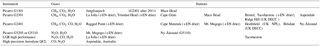
One of the strengths of AGAGE is its dependence upon well-defined internal absolute gravimetric calibration procedures that can be repeated periodically to ensure the accuracy of the long-term measured trends. During the period of AGAGE there have been seven absolute primary calibration efforts, SIO-93, SIO-98, SIO-05, SIO-07, SIO-12, SIO-14, and SIO-16, named after the SIO laboratory and the year in which the scale was completed. The “bootstrap” methods used to prepare primary gravimetric standards at ppt levels and the way in which these standards are integrated to define a calibration scale are described in the AGAGE “history paper” (Prinn et al., 2000). The methods used to propagate these scales to the species measured by the Medusa GC-MS are discussed by Miller et al. (2008). At present, ambient-level SIO primary calibration scales have been prepared for 42 AGAGE species: N2O, PFC-14 (CF4), PFC-116 (C2F6), PFC-218 (C3F8), PFC-318 (c-C4F8), PFC-3-1-10 (C4F10), PFC-4-1-12 (C5F12), PFC-5-1-14 (C6F14), PFC-6-1-16 (C7F16), PFC-7-1-18 (C8F18), SF6, SF5CF3, SO2F2, NF3, HFC-23, HFC-32, HFC-125, HFC-134a, HFC-143a, HFC-152a, HFC-227ea, HFC-236fa, HFC-245fa, HFC-356mfc, HFC-43-10mee, HCFC-22, HCFC-141b, HCFC-142b, CFC-11, CFC-12, CFC-113, CFC-114, CFC-115, Halon-1211, Halon-1301, Halon-2402, CH3Br, CH3Cl, CH2Cl2, CHCl3, CH3CCl3, and CCl4. Among them, NF3, C4F10, C5F12, C6F14, C7F16, and C8F18 were calibrated by the method of internal additions, which is by spiking real air with gravimetrically determined amounts of the analyte (Arnold et al., 2012), while the remaining gases were calibrated by the conventional AGAGE method of adding gravimetrically determined amounts of the analytes to analyte-free artificial “zero air”. For CF4, the primary calibrations have been made both ways with excellent agreement. For the volatile gases like CF4 and NF3, the use of the internal additions method is particularly valuable to avoid biases in their separation or detection due to interferences from the presence of krypton and other inert gases in real air but not in artificial zero air. The precisions of these calibration scales, based on the internal consistency among the individual primary standards, range from about 2 % for the least abundant compounds to < 0.1 % for the more abundant compounds. The absolute accuracies of these scales, based on estimates of maximum systematic uncertainties, including the purities of the reagents used in their preparation and possible systematic analytical interferences, are between 0.3 and 2 % greater than the statistical uncertainties depending on the compound and its atmospheric abundance.
The evolution of GC-MS techniques in AGAGE has greatly increased the number of species that are measured in the program and has thus exceeded, at least temporarily, our capacity to prepare and maintain gravimetric primary calibration scales. To bridge this gap and, very importantly, to decouple the long-term measurement program for the evolving and independent primary calibration process, AGAGE has adopted a relative calibration scale for all Medusa and GC-MD measurements. This scale, designated R1, is defined by regular intercomparisons of trace gas concentrations in a suite of whole-air secondary (“gold”) tanks maintained at the SIO laboratory. These tanks are compared against each other to assess possible drift and against primary standards for those species for which we have primary standard calibrations. Every year, this suite of secondary tanks is extended with at least one new tank filled under clean air conditions in winter or spring and the intercomparison is repeated. Other tanks filled at the same time are calibrated against this suite of tanks and sent to each station as calibration “tertiary” standards, where they are either directly measured (GC-MD) or used to calibrate working “quaternary” standards (Medusa) at each measurement site. As primary calibration scales evolve at SIO, NOAA/ESRL, Bristol, Empa, NCAR, NIES, or any other laboratory, the relationships of their scales to the R1 scale can be measured to obtain a set of factors by which our R1 values can be multiplied to report Medusa data on any of these calibration scales. The R1 scale is flexible to designate tanks other than R1 as a reference tank for individual compounds, which were not present at sufficient concentrations or were not measured in the original R1 tank. Looking to the future, this enables us to keep pace with the changing atmospheric concentrations of many species and to incorporate corrections for possible nonlinearities in the calibration process and for possible drifts in standard mixtures. This technique has been used to provide calibrations for species not on an SIO scale such as CFC-13 (METAS-2017), CHBr3 (NOAA-2009P), PCE (NOAA-2003B), and HCFC-133a (Empa-2013; Vollmer et al., 2015c).
AGAGE gravimetric calibration activities are independent from those in other laboratories (except for the CO2 calibrations used in the bootstrap method that come from the Keeling laboratory at SIO), but there are also strong synergies, especially with NOAA/ESRL. For example, the SIO-14 calibrations showed excellent agreement with NOAA for Halon-2402 (Vollmer et al., 2016), while AGAGE atmospheric CH2Cl2 mole fractions based on the SIO-14 scale are significantly higher than those reported by NOAA (Carpenter et al., 2014). This subject of intercalibration is discussed further in Sect. 3.2.
Whole-air and synthetic mixture calibration standards used in AGAGE are stored in 34 L high-pressure (60 bar) electropolished stainless steel canisters designed at SIO and manufactured by Essex Industries© that are legal for international shipment. Although the adoption of a single primary calibration scale from a central calibration facility for each measured species has been advocated by some researchers, AGAGE does not favor this approach. The existence of more than one independent high-precision traceable calibration scale for each measured species, with frequent intercomparisons among independently calibrated field measurements (see Table 5, Sect. 3.2) and with direct intercomparison of the calibration standards themselves (Hall et al., 2014), reduces vulnerability to systematic errors and long-term calibration drifts for all participating primary calibration and measurement programs.
Table 5Scale conversion factors between NOAA and AGAGE (SIO) expressed as a NOAA ∕ AGAGE ratio based on a comparison of NOAA/ESRL/GMD flask data to AGAGE in situ data at common sites. For CH4, N2O, and SF6, NOAA flask data from the carbon cycle and greenhouse gases (CCGG) group have been used; for all other species NOAA flask data from the halocarbons and other atmospheric trace species (HATS) group are used. The respective scales used in each network are indicated in the table along with the instrumental method used for the analysis. The sites used in the comparisons are listed in column five, followed by the length of the comparison period. Lastly, comments on the consistency of the comparisons for each species are given.
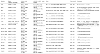
Table notes: comparisons between NOAA HATS data and AGAGE in situ
were performed based on the NOAA data posted on the ftp site:
ftp://ftp.cmdl.noaa.gov/hats/ (last access: 21 May 2018).
GC-MS-ADS Med indicates data from the ADS instruments at Cape
Grim and Mace Head used from 1998–2003, with Medusa data used from 2004
onwards at the sites indicated.
GC-ECD–GC-MS Med indicates a
combined data record from the GC-ECD (GC-MD) instruments with the GC-MS
Medusa data used for the latter part of the record.
Sites: CGO
– Cape Grim, Australia; SMO – Cape Matatula, Samoa; RPB – Ragged Point,
Barbados; THD – Trinidad Head, USA; MHD – Mace Head, Ireland; ZEP –
Zeppelin Mountain, Ny-Ålesund, Norway.
Some species are
measured by multiple instruments and/or flask samples; selected results shown
here.
2.7 Primary and affiliate station facilities and infrastructure
While the individual station size and infrastructure varies depending on their location and the presence of other complementary gas and aerosol measurement programs, all stations consist of permanent buildings (wood, concrete, steel, fiberglass) with air samples drawn using non-contaminating pumps through lines with inlets located on adjacent high towers. The details about the general air sampling setup for each instrument are provided in Miller et al. (2008) and Prinn et al. (2000). The sampling lines are either stainless steel or layered polyethylene–aluminum–Mylar (Dekabon© or Synflex©). For more information on individual stations, we refer the reader to the AGAGE website (http://agage.mit.edu (last access: 21 May 2018). All stations (except Hateruma and Cape Ochiishi) periodically exchange stainless steel on-site Essex calibration tanks (tertiary standards) calibrated at SIO linking the measurements to the AGAGE SIO primary and secondary standards. Some stations also use modified RIX© oil-free air compressors and the tertiary standards to prepare quaternary standards either on-site, in their home laboratories, or supplied by SIO to extend the lifetime of the tertiary standards. At Cape Grim and Ny-Ålesund, the quaternary standards are prepared by a cryogenic collection of whole air with subsequent ejection of condensed water.
2.8 Secondary stations
In addition to the primary and affiliate stations in AGAGE, there are complementary secondary stations, usually at either more polluted urban locations or at more remote sites that share some or all of the AGAGE technology and calibrations.
SIO carries out continuous measurements of all AGAGE gases in La Jolla in conjunction with its extensive calibration (Sect. 2.6) and instrument development operations.
The University of Bristol runs the UK DECC (Deriving Emissions related to Climate Change) network of tall towers at Ridge Hill, Angus (now decommissioned), Tacolneston (in collaboration with the University of East Anglia), Heathfield (UK National Physical Laboratory), and Bilsdale in the UK measuring CO2, CO, CH4, N2O, and SF6 and linked to the AGAGE Mace Head station and to AGAGE calibrations and some technologies. Tacolneston also includes measurements of H2 and CO via MRD and a Medusa GCMS.
CSIRO is operating two Medusa GCMSs at Aspendale, and Picarro CRDS CH4 and CO2 (and CO at one station) instruments at Burncluith (26∘ S, G2401), Ironbark (27∘ S, G2301), Aspendale (38∘ S, G2301), Macquarie Island (55∘ S, G2301), Casey Station, Antarctica (66∘ S, originally a G1301 now replaced by a G2301), and onboard the new CSIRO research vessel the RV Investigator (G2301). Picarro CRDS CH4 and CO2 instruments were also previously operated at Gunn Point, northern tropical Australia (11∘ S, G1301, 2010–2017, currently suspended), Arcturus (22∘ S, G1301 replaced by G2301, 2010–2014), and Otway (38∘ S, ESP1000, 2009–2012). CSIRO is also operating high-precision Aerodyne Research QCL systems for CO and N2O and another for the stable isotopes of CO2 at Aspendale. All of these instruments are configured to run with AGAGE–GCWerks software (see Sect. 3.3).
2.9 Air archives
CSIRO has been collecting and archiving pressurized 34 L electropolished canisters of cryo-trapped air collected during clean air conditions at Cape Grim since the mid-1970s, and plans to continue into the future (Fraser et al., 2017). This “Southern Hemisphere air archive” has proven to be an invaluable resource to the international atmospheric chemistry community, including AGAGE, because a wide range of species that could not be measured at the time of collection can be measured retrospectively in the archive as long as those species are conserved in these canisters. Until 2013 a target of four Cape Grim air archive samples were collected each year, while from 2014 onwards six air archive tanks are collected each year. Measurements from this Southern Hemisphere archive have made significant contributions to several recent AGAGE papers by addressing the following: HFC-23 (Miller et al., 2010); PFCs (Mühle et al., 2010; Trudinger et al., 2016); SF6 (Rigby et al., 2010); CFC-13, CFC-114, and CFC-115 (Vollmer et al., 2018); Halon-1211, Halon-1301, and Halon-2402 (Vollmer et al., 2016); and HFC-365mfc, HFC-245fa, HFC-227ea, and HFC-236fa (Vollmer et al., 2011). There was a parallel “Northern Hemisphere archive” collected by Rei Rasmussen at Cape Meares, Oregon during the ALE and GAGE programs, but these samples are no longer accessible to this program and are mostly used up. The SIO AGAGE group has been storing a Northern Hemisphere archive of air compressed at Trinidad Head and La Jolla since the mid-1990s and has collected a series of Northern Hemisphere air samples from various sources (e.g., SIO laboratories of Charles D. Keeling and Ray F. Weiss, NOAA-GMD, and NILU) and of varying integrity for trace gas measurements that extends this record back to the early 1970s. Measurements from this Northern Hemisphere archive have made significant contributions to several recent AGAGE papers, especially for more inert species such as the PFCs, NF3, and SF6 (e.g., Mühle et al., 2009, 2010; Rigby et al., 2010; Weiss et al., 2008; Arnold et al., 2013).
Additional air archive samples used in AGAGE studies were derived from firn air collections in Greenland and Antarctica obtained by international consortia. The AGAGE analyses of firn air used Medusa GC-MS instruments and substantially extended mole fraction data back in time along with emission estimates derived from the data, specifically for Halons (Vollmer et al., 2016), PFCs (Trudinger et al., 2016), and minor CFCs (Vollmer et al., 2018).
In this section, the seven subsections address the following: meteorological interpretation of data (Sect. 3.1), data intercomparisons (Sect. 3.2), flux estimation using data and models (Sect. 3.3), and flux estimation using 3-D Eulerian models (Sect. 3.4), 3-D Lagrangian models (Sect. 3.5), merged 3-D Eulerian and Lagrangian models (Sect. 3.6), and simplified (2-D) models (Sect. 3.7).
3.1 Meteorological interpretation
As part of processing the AGAGE data, we place an identification flag on each measured value in an attempt to separate regional and/or local pollution events from background measurements. The current, objective (statistically based) algorithm has been successfully implemented and uniformly applied to the entire ALE/GAGE/AGAGE time series including data from all AGAGE primary and affiliate stations (except Hateruma and Cape Ochiishi) and all instruments (GC-MS, GC-MD, Picarro). Moreover, the algorithm has been designed to be easily reapplied to the entire dataset in the event of (minor) modifications to the algorithm. The concept of the algorithm is to examine the statistical distributions of 4-month bins of measurements (approximately 4320 GC-MD or 1440 Medusa GC-MS values) of any species at a specified site and centered on one day at a time after removing the trend over the period (O'Doherty et al., 2001; Cunnold et al., 2002). The algorithm can be applied to the results from 3-D models to separate the background and polluted values (Ryall et al., 2001; Simmonds et al., 2005). We also use a 3-D Lagrangian back-trajectory model driven by reanalyzed meteorology, specifically the UK Met Office's Numerical Atmospheric dispersion Modelling Environment (NAME; Ryall et al., 1998; Jones et al., 2007), to further evaluate the statistical pollution algorithm (O'Doherty et al., 2001; Cunnold et al., 2002) and include this evaluation as part of the pollution and background identification flag associated with each measurement. NAME is Lagrangian (Sect. 3.5). In NAME, large numbers of particles at the station are effectively advected backwards in time by 3-D reanalysis meteorological fields, with turbulent dispersion represented by a random walk technique. Particles first encountering the surface or surface boundary layer in known trace-gas-emitting regions are then flagged as polluted. An observation is also considered potentially polluted if the atmosphere at the station is stable with very low winds and known nearby trace gas sources. NAME back trajectories are automatically computed for every AGAGE measurement and used extensively in the semiannual AGAGE data reviews.
3.2 Data intercomparisons
AGAGE cooperates with other groups carrying out flask sampling and/or in situ real-time tropospheric measurements in order to produce harmonized global datasets for use in modeling. Toward this end, AGAGE routinely collaborates with NOAA/ESRL/GMD to develop best estimates of the differences in absolute calibrations and field site calibrations between them and the AGAGE–SIO scales (see Elkins et al., 2015, and the NOAA/ESRL/GMD website for the NOAA/ESRL/GMD database). This is undertaken in several ways: comparisons involving exchanges of tanks (checking absolute calibration); comparisons of hemispheric and global mean trends estimated by the two networks; examination of differences between the AGAGE and GMD in situ instruments at our common in situ site, Cape Matatula (checking the propagation of standards to remote sites); and ongoing extensive comparisons between AGAGE in situ GC-MD and GC-MS data and GMD flask data at the six AGAGE sites where GMD flasks are filled (Zeppelin, Mace Head, Trinidad Head, Ragged Point, Cape Matatula, and Cape Grim), with the results reported at the semiannual AGAGE meetings. To help ensure progress on this and other cooperative endeavors, leaders and members of the relevant NOAA/GMD group regularly attend the semiannual AGAGE meetings; other joint meetings with GMD personnel are held from time to time. Examples of the scale conversion factors determined from the comparison of AGAGE in situ data to NOAA flask results are given in Table 5. There is generally good consistency with time for these with some exceptions, most notably CCl4. The CCl4 comparison shows a trend with time from around 3.5–4.0 % in 1995–2000 to approximately 1.5 % in 2013–2017. Because these factors are updated when additional intercomparisons occur, we advise data users to consult the AGAGE website (http://agage.mit.edu, last access: 21 May 2018) for possible updates.
Also, comparisons between AGAGE in situ GC-MD and GC-MS data at Cape Grim and flask data from other groups (CSIRO, NIES, U. East Anglia, SIO, U. Heidelberg, Max Planck Inst. Mainz) have been and continue to be made. Exchanges of tanks between the collaborating NIES group and AGAGE–SIO are also performed to compare absolute calibrations. Also, there are routine data intercomparisons carried out within AGAGE for those gases measured on both the AGAGE Medusa GC-MS and AGAGE GC-MD instruments. Finally, three AGAGE sites (SIO, Mace Head, and Cape Grim) participated in the WMO-organized IHALACE (International HALocarbon in Air Comparison Experiment), round robin intercomparisons (Hall et al., 2014).
3.3 Flux estimation using measurements and models
A major goal of AGAGE is to estimate surface fluxes and/or atmospheric sinks (lifetimes) of trace gases by merging measurements and models using advanced statistical methods (Prinn et al., 2000; Weiss and Prinn, 2011). Specifically, we use a range of Bayesian methods, in which a priori estimates of atmospheric sinks and surface fluxes (or uncertain parameters in flux models) are adjusted to improve agreement with the trace gas observations within estimated uncertainties, and it is important to ensure that the problems are well posed, that the ill-conditioning inherent in our emission estimations is minimized, and that model and measurement imperfections are accounted for properly (e.g., Prinn, 2000; Tarantola, 2005). A basic requirement for all our inverse schemes is an accurate and realistic atmospheric chemical transport model (CTM). Even small transport errors can lead to significant errors in estimated sources or sinks (Hartley and Prinn, 1993; Mahowald et al., 1997; Mulquiney et al., 1998). We use a range of CTMs to estimate trace gas budgets at different spatial scales: two-dimensional “box” models provide global source and sink estimates using baseline observations, global three-dimensional Eulerian models are used for estimating fluxes at national to continental scales, and high-resolution regional Lagrangian models provide fine-scale source estimations close to AGAGE monitoring sites.
Here, and in Sect. 3.4–3.7, we summarize the methods and models actually used by AGAGE scientists to interpret AGAGE measurements. There are alternative methods and models that may give differences in estimated emissions, especially at regional scales. The AGAGE publications generally address the issue of differences, if any, between the estimated emissions and those reported in prior studies by other non-AGAGE scientists. Some of these alternative methods are addressed in Sect. 4.6 and 4.8, but it is beyond the scope of this paper to review all the alternatives. Instead we refer the reader to two comprehensive books that provide in-depth summaries of most of the major models and methods used to estimate sources and sinks from measurements (Enting, 2002; Kasibhatla et al., 2000).
We relate the vector of measured atmospheric mole fractions (y) to emissions or initial conditions in a “parameters vector” (x) using the “measurement” equation . Here H is a matrix of sensitivities, or partial derivatives, of simulated measurements in y (= Hx) to each element in x and is derived using the CTMs; e describes the random component of the error due to errors in the measurements and in the CTM. These errors form the error covariance matrix R. A prior estimate of x (xprior) is generally needed, with uncertainties contained in the error covariance matrix Pprior. Formally, since the chemical lifetime for a reactive trace gas can depend on emissions of that gas, then H=H(x) so the equation y=Hx is nonlinear in x. For many ozone-depleting and greenhouse gases this nonlinearity is negligibly weak and is ignored. Exceptions exist, as discussed later. There are a number of statistical approaches that have been developed and implemented to make these estimations (e.g., Kasibhatla et al., 2000; Prinn, 2000; Rigby et al., 2011; Ganesan et al., 2014).
A common Bayesian statistical approach is “optimal estimation” (e.g., Kasibhatla et al., 2000) in which one minimizes a “cost” function (J) that is the sum of two quadratic forms: () that minimizes the weighted difference between measured and modeled mole fractions and () that minimizes the weighted difference between the estimated parameters and their prior. This minimization yields analytical solutions to ), , and the “gain” matrix . Examples of this approach using global 3-D Eulerian models are provided by Chen and Prinn (2005, 2006) for CH4, Xiao et al. (2010a) for CH3Cl, Xiao et al. (2010b) for CCl4, Rigby et al. (2010, 2011) for SF6, Saikawa et al. (2012, 2014b) for HCFC-22, and Huang et al. (2008) and Saikawa et al. (2014a) for N2O. Weak nonlinearities may occur when lifetimes vary with emissions (e.g., OH depends on CO and CH4 emissions). This problem can be addressed by recalculating the time-dependent partial derivative (sensitivity) H matrix after inversion of all the data and then repeating the inversion with the new H matrix to ensure convergence (Prinn, 2000).
Random measurement imperfections are associated with in situ instrument precision, satellite retrieval errors, and inadequate sampling in space and time. If known, random model errors can also be incorporated into the model–measurement error covariance matrix (R). It is also important to recognize that correlated model–measurement errors, which comprise R, and errors in the prior contained in Pprior are often poorly known quantities. Ganesan et al. (2014) explicitly allow such uncertainties to be derived in the inversion to minimize the effect of subjective assumptions on derived fluxes. This hierarchical Bayesian method (Ganesan et al., 2014) incorporates “hyper parameters” that describe the model–measurement and/or prior uncertainty covariance matrices (R and P) in the inversion. This approach leads to solutions that are less sensitive to the (often subjective) assumptions that are required about uncertainties in traditional Bayesian approaches. The hierarchical inversion scheme cannot, in general, be solved analytically, and therefore Markov chain Monte Carlo (MCMC) methods must be applied to that sample from the posterior distribution using a large number (∼ 104–105) of realizations of the parameter space (e.g., Rigby et al., 2011). Recently, this MCMC approach has been extended to include problems in which the dimension of the parameter space is itself considered unknown using a so-called “reversible jump” MCMC algorithm (Lunt et al., 2016). This method has been applied to high-resolution regional inversions using a Lagrangian model to sample from a range of possible basis function decompositions of the flux space, objectively determining the level of decomposition that is appropriate to effectively minimize “aggregation error” (i.e., an inflexibility in the space that could lead to errors in the prior distribution unduly influencing the outcome of the inversion; Kaminski et al., 2001), while maintaining an acceptable level of uncertainty reduction.
We also address model structural errors and random and systematic transport errors (i.e., errors in H) through the utilization of multiple model versions (Locatelli et al., 2013) and Monte Carlo methods (Prinn et al., 2001, 2005; Huang et al., 2008). The Monte Carlo methods also include systematic errors in measurement calibration.
For the determination of the regional sources of trace gases, beginning with Chen and Prinn (2006) we now frequently merge measurements from the AGAGE and NOAA/ESRL/GMD stations and also aircraft and satellites whenever appropriate (e.g., Ganesan et al., 2017). Because source and sink estimation is very sensitive to errors in time and space gradients, we ensure intercalibration among instruments of the same type and intercomparison between different instruments measuring the same quantity. We also objectively determine the accuracy and precision of each measurement when combining data, since data are weighted inversely to their variances (contained in R). Nonzero values for the off-diagonal elements of R and P can occur. Because the AGAGE measurement stations are well separated, off-diagonal elements (covariances) of R should be much smaller than the diagonal elements (variances) and are usually ignored. Also, P element covariances should be much smaller than the variances except when state vector elements are correlated, which can be avoided when choosing the elements. These covariances (off-diagonal elements of P) are discussed in the individual papers where they are relevant.
3.4 Flux estimation using 3-D Eulerian models
For our inverse studies we initially used the 3-D MATCH of the National Center for Atmospheric Research, NCAR (Mahowald et al., 1997; Rasch et al., 1997; Lawrence et al., 1999). MATCH was driven by data from the NCEP, ECMWF, and GSFC/NASA/DAO reanalyses (Rasch et al., 1997; Mahowald et al., 1997). Subgrid mixing processes, which include dry convective mixing, moist convective mixing, and large-scale precipitation processes, were computed in the model. MATCH was used at a horizontal resolution as fine as T62 (1.8∘ × 1.8∘), with either 42 or 28 levels in the vertical. Utilizing MATCH with AGAGE, ESRL, and other data, we estimated monthly regional and global emissions for many AGAGE species (e.g., Chen and Prinn, 2005, 2006; Huang et al., 2008; Xiao et al., 2010a, b). The ability of MATCH to accurately simulate the effects of transport on long-lived trace gases is well illustrated by CH4 simulations (Chen and Prinn, 2005). The need to use reanalysis meteorology in MATCH that captures the actual circulation was evident from the observed CH3CC13 seasonal cycle at the tropical South Pacific station (Samoa) that showed remarkable sensitivity to the El Niño–Southern Oscillation (ENSO). This sensitivity was attributed to the modulation of cross-equatorial transport during the Northern Hemisphere winter by the interannually varying upper tropospheric winds in the equatorial Pacific; this was a previously unappreciated aspect of tropical atmospheric tracer transport (Prinn et al., 1992).
More recently we use the newer NCAR Model for Ozone and Related Tracers (MOZART) that also simulates global three-dimensional mole fractions of atmospheric trace species (Emmons et al., 2010). Like MATCH, MOZART can be run off-line and driven by a variety of state-of-the-art reanalysis meteorological fields, including the National Center for Environmental Prediction/NCAR reanalysis (Kalnay et al., 1996) and the NASA Modern Era Retrospective Analysis for Research and Applications, NASA-MERRA (Bosilovich et al., 2008). We have specifically used MOZART inversions to estimate regional emissions for SF6 (Rigby et al., 2010), heavy PFCs (Ivy et al., 2012a, b), HCFC-22 (Saikawa et al., 2012, 2014b), and N2O (Saikawa et al., 2014a).
3.5 Flux estimation using 3-D Lagrangian models
Another modeling approach that we have used utilizes air histories or “footprints” computed from Lagrangian models driven by analyzed observed winds. These air histories, computed over a predefined region, quantify the time and locations that air masses have interacted with the surface (and therefore fluxes from the surface) prior to measurement at a station. Using this information and the measurements, we can solve for fluxes from these predefined regions. The method requires accurate simulation of both advective back trajectories and diffusion. We had examined earlier the use of the HYSPLIT model (Draxler and Hess, 1997) for this purpose (Kleiman and Prinn, 2000), and now we also use additional Lagrangian particle dispersion models (LPDMs). In particular, the LPDM NAME of the UK (Ryall et al., 1998) has been used to determine source strengths for observed species on regional scales (e.g., Cox et al., 2003; O'Doherty et al., 2004, 2009; Reimann et al., 2005; Derwent et al., 2007; Ganesan et al., 2015; Manning et al., 2011; Rigby et al., 2011; Lunt et al., 2015). The LPDM FLEXPART has also been applied to the inversion of AGAGE data for several species (Stohl et al., 2009, 2010; Maione et al., 2014; Graziosi et al., 2015, 2016, 2017; Fang et al., 2014).
3.6 Flux estimation using merged Eulerian and Lagrangian models
Given the high-frequency nature of the AGAGE measurements, we can extract a great deal of information on sources close to the monitoring sites. LPDMs like NAME have the useful property that they directly calculate the sensitivity of the measurements to emissions from every grid cell in the domain. However, one limitation of these models is that boundary conditions must be specified or estimated (e.g., Stohl et al., 2009). In contrast, inversions using global Eulerian CTMs, such as MOZART, do not usually require boundary conditions but can only estimate emissions from a limited number of regions (unless an adjoint model of the CTM is available; Meirink et al., 2008). In addition, these models are sensitive to uncertainties in species lifetimes.
To combine the Eulerian and Lagrangian approaches, we can decompose the sensitivity matrix H into components that represent the sensitivities of the observations to initial conditions (HIC), emissions from model grid cells close to AGAGE stations (HLE), and emissions from aggregated regions that are farther from the AGAGE sites (HNLE): H=(HIC, HNLE, HLE; Rigby et al., 2011). HIC and HNLE can be estimated using the Eulerian model at reasonable computational cost, while the term HLE can be determined using the Lagrangian model. Consideration must be made of the fate of emissions close to AGAGE sites that leave the LPDM region and gradually become mixed into the global atmosphere. HLE must therefore be decomposed into a short-timescale term HLE,LAM, for which the Lagrangian model is used, and a long-timescale term HLE,EUM, which can be approximated using the Eulerian model. Once H is constructed, the inversion can be solved using any Bayesian inverse method incorporating measurement, model, and state error covariance matrices (Sect. 3.4). This approach has the advantage over previous global emissions estimates that only used an LPDM in that constant background mole fractions do not have to be assumed (e.g., Stohl et al., 2009). Further, by solving for regional and global emissions and covariance in a single step, we can avoid many of the problems encountered in two-step “nested” inverse methods (e.g., covariance between emissions in the “Lagrangian region” and those outside, as in the method of Rödenbeck et al., 2009).
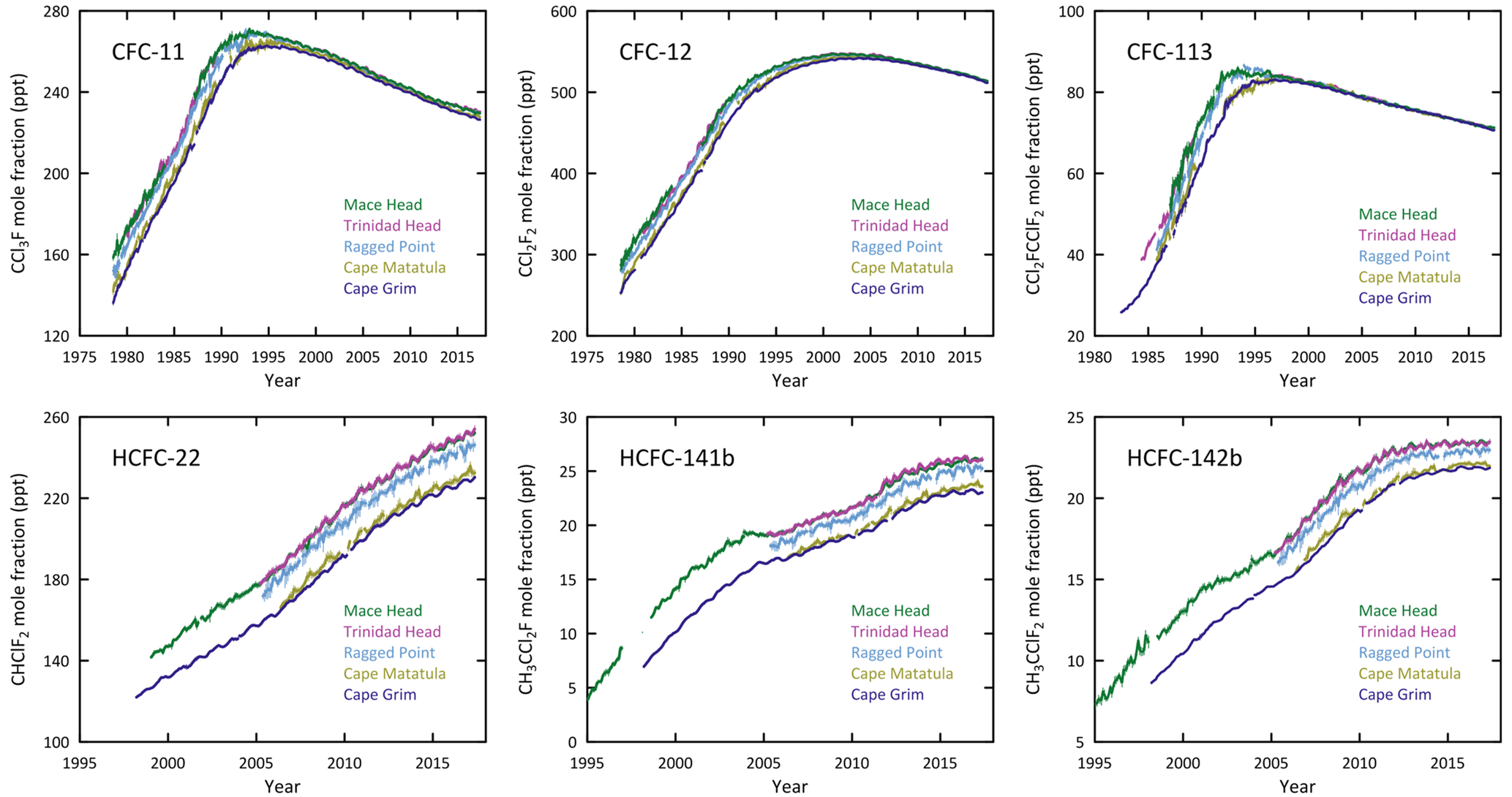
Figure 3Monthly mean mole fractions (ppt) and their standard deviations (vertical bars) for selected AGAGE Montreal Protocol gases through 2017.
Inverse estimates of global sulfur hexafluoride (SF6) emissions have been carried out using this method (Rigby et al., 2011). The derived global total emission rate agrees well with previous CTM-based estimates by Rigby et al. (2010), and the regional emissions qualitatively agree with their findings.
3.7 Application of simplified models
The 3-D models, being computationally expensive, do not always lend themselves well to doing very long time integrations and multiple runs to address uncertainty (e.g., thousands of runs for Monte Carlo treatments of model, rate constant, and absolute calibration errors). Therefore, 2-D models have been widely used to analyze long-term trends in AGAGE data. The AGAGE 12-box model (Cunnold et al., 1994; Prinn et al., 2001, 2005; Rigby et al., 2013, 2014) uses transport parameters that have been “tuned” using AGAGE observations of trace gas trends and latitudinal gradients (e.g., Cunnold et al., 1994; Rigby et al., 2013) so that the model can simulate monthly mean observations at background AGAGE stations with pollution events removed. From these simulations, multi-decadal AGAGE time series have been used to estimate trace gas global emissions and atmospheric lifetimes. For example, this 2-D model has been used to estimate emissions of three light PFCs (PFC-14, PFC-116, and PFC-218; Mühle et al., 2010) and NF3 (Arnold et al., 2013), and combined with the 3-D MATCH has provided estimates of the influence of model errors on overall emission uncertainties for N2O (Huang et al., 2008). A more simplified three-box 2-D model has also been employed to simultaneously estimate CH3CCl3 and CH4 lifetimes and emissions using AGAGE observations of interhemispheric differences and growth rates (Rigby et al., 2017).
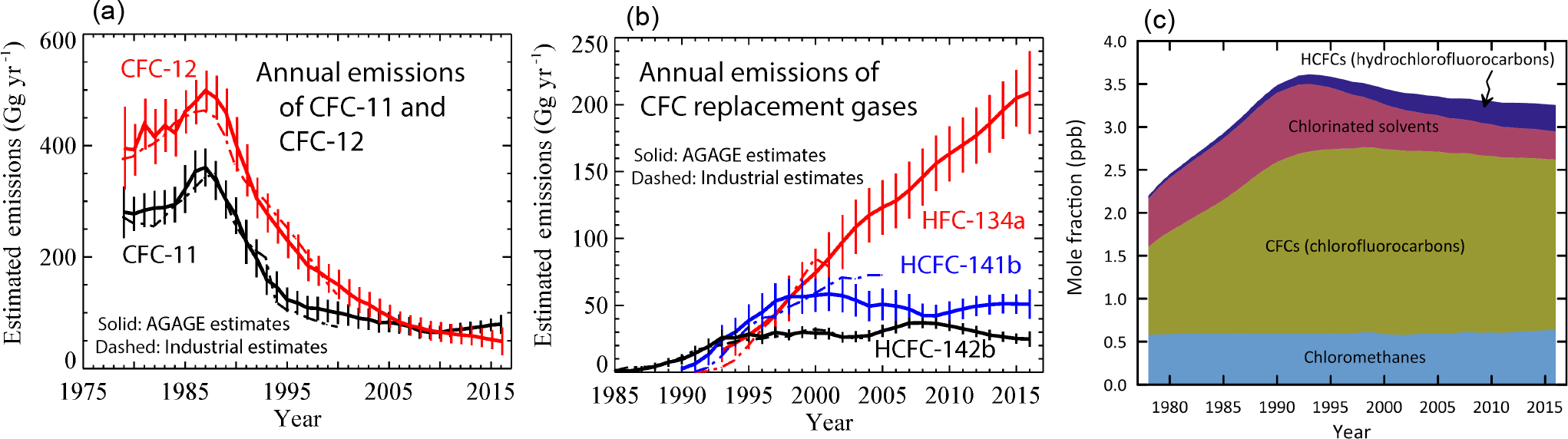
Figure 4Inversely estimated emissions using our Bayesian statistical approach (Sect. 3.3) and our 12-box model (Sect. 3.7) of the following: selected AGAGE regulated gases (a) and selected AGAGE replacement gase (b) compared to estimates from industrial, national, and/or UNEP reports. Estimates of total tropospheric chlorine from all AGAGE data (c; chlorinated solvents are CCl4 and CH3CCl3; chloromethanes are CH3Cl, CH2Cl2, and CHCl3; see Table 1 for a full list of AGAGE chlorine-containing compounds).
In this section, the nine subsections discuss the following: trends in Montreal Protocol gases and their replacements (Sect. 4.1), whether the Montreal Protocol is working (Sect. 4.2), trends in Kyoto Protocol gases (Sect. 4.3), the recent rise of powerful synthetic greenhouse gases (Sect. 4.4), trends in radiative forcing (Sect. 4.5), the determination of OH concentrations using models and multiple gases (Sect. 4.6), AGAGE emission estimates for all gases (Sect. 4.7), emission estimates from multiple networks, measurement platforms and alternative models (Sect. 4.8), and tabulation and access to AGAGE publications (Sect. 4.9). We focus on the greenhouse and ozone-depleting gases in this section, but note that the four non-methane hydrocarbons listed in Table 1 (ethane, propane, benzene, toluene) are optional compounds measured at some of the stations (for examples, see Yates et al., 2010; Grant et al., 2011; Derwent et al., 2012; Lo Vullo et al., 2016a, b). Also, CO and H2 are measured at two stations (e.g., Xiao et al., 2007). When correlated with the other gases in Table 4, these species can be used as indicators of the sources of these other gases, and they are all also relevant to the fast photochemistry of OH.
4.1 Trends in Montreal Protocol gases and their replacements
The Montreal Protocol on Substances that Deplete the Ozone Layer, enacted to protect the ozone layer, regulates many ozone-depleting gases for the primary purpose of lowering stratospheric chlorine and bromine concentrations. From AGAGE measurements (Fig. 3), two of the major CFCs (CFC-11, CFC-113) have both been decreasing in the atmosphere since the mid-1990s. While their emissions have decreased very substantially in response to the Montreal Protocol, their long lifetimes of around 50 and 90 years, respectively, mean that their sinks can reduce their levels only at about 2 and 1 % per year, respectively. The other major CFC (CFC-12) has a somewhat longer lifetime (about 100 years) and a slower phase-out of emissions, and consequently its atmospheric levels have reached a plateau more recently and are now decreasing.
The three major HCFCs (HCFC-22, HCFC-141b, and HCFC-142b) are replacements for the CFCs and have continued to rise in recent years. The rates of rise decreased somewhat in the late 1990s for HCFC-141b (9-year lifetime) and HCFC-142b (18-year lifetime), which is consistent with decreases in their emissions from developed countries. They then increased again. which is consistent with increases in developing country emissions. In contrast, rates of rise have slowly declined post-2008 for HCFC-22 (12-year lifetime). AGAGE mole fraction data and derived emissions from a wide range of ozone-depleting species have been published in multiple recent papers (Fraser et al., 2014; Graziosi et al., 2015, 2016; Keller et al., 2011; Kim et al., 2010, 2012; Li et al., 2011, 2014; Lunt et al., 2015; Maione et al., 2013, 2014; Miller et al., 1998; Rigby et al., 2013; Saikawa et al., 2012, 2014b; Stohl et al., 2010; Vollmer et al., 2016, 2017; Xiang et al., 2014; Xiao et al., 2010b).
4.2 Is the Montreal Protocol working?

Figure 5Monthly mean mole fractions and standard deviations for selected Kyoto Protocol gases through 2017.
The global abundance of tropospheric chlorine and emissions, via inverse methods, of ozone-depleting gases are estimated from AGAGE measurements (Fig. 4). Some specific conclusions are as follows.
-
International compliance with the Montreal Protocol is so far resulting in CFC and chlorocarbon abundances comparable to the target levels – the Protocol is working although estimated global CFC-11 emissions post-2010 are rising (Fig. 4), but the method used does not provide the regional-level emission estimates needed to identify the causes of this rise. Montzka et al. (2018) recently concluded that East Asia was the source.
-
The abundance of total chlorine in long-lived CFCs and other chlorocarbons (CFC-11, CFC-12, CFC-13, CFC-113, CFC-114, CFC-115, HCFC-22, HCFC-141b, HCFC-142b, CHCl3, CH3CCl3, CH3Cl, CCl4, CH2Cl2, CCl2CCl2) in the lower troposphere reached a maximum of about 3.6 ppb in 1993 and is beginning slowly to decrease in the global lower atmosphere driven initially by CH3CCl3 and later by CFC decreases (note that CH3Cl, CH2Cl2, and CCl2CCl2 are not regulated in the Montreal Protocol, yet CH2Cl2 is increasing).
-
The CFCs have atmospheric lifetimes consistent with destruction in the stratosphere being their principal removal mechanism.
-
Multi-annual variations in measured CFC, HCFC, HFC, and other chlorocarbon emissions deduced from ALE/GAGE/AGAGE data are approximately consistent with variations estimated independently from industrial production and sales data where available. HCFC-141b shows the greatest discrepancies. The processes producing the deduced CCl4 emissions are not fully understood. The 2010 and 2014 WMO Scientific Assessments of Ozone Depletion noted that emissions of CCl4 inferred from AGAGE and NOAA observations were substantially higher (∼ 50 Gg yr−1) than estimates based on consumption reported to UNEP (Montzka et al., 2011a; Carpenter et al., 2014). Recent studies have attempted to reevaluate the global CCl4 budget (Liang et al., 2017). Estimates of the soil and ocean partial lifetimes have been revised upward (Rhew and Happell, 2016; Butler et al., 2016) and several new industrial sources have been identified (Sherry et al., 2017), substantially reducing the gap between top-down and bottom-up estimates (Chipperfield et al., 2016).
-
The mole fractions of the HCFCs, which are interim replacements for CFCs, rose very rapidly in the atmosphere until the early 2000s, but are now only rising relatively slowly; the exception is HCFC-22, which has been in use almost as long as the CFCs. HCFC-22 continues to increase rapidly in the atmosphere and contributes significantly to atmospheric chlorine loading.
-
The mole fractions of HFCs, which are long-term replacements for CFCs and HCFCs, continue to rise rapidly in the atmosphere and are the major Kyoto synthetic greenhouse gases contributing to increased radiative forcing. They were added to the Montreal Protocol in the 2016 Kigali Amendment.
AGAGE scientists, AGAGE data, and AGAGE modeling results played a prominent role in all the WMO-UNEP Ozone Assessments, most recently the WMO-UNEP 2010 (Montzka et al., 2011a) and WMO-UNEP 2014 (Carpenter et al., 2014) Ozone Assessments, also providing many coordinating and lead authors, coauthors, contributing authors, and reviewers. The AGAGE-led paper on the reevaluation of the lifetimes of the major CFCs and CH3CCl3 using atmospheric trends (Rigby et al., 2013) was an important input into the 2014 Ozone Assessment (Carpenter et al., 2014).
4.3 Trends in Kyoto Protocol gases
The Kyoto Protocol, followed now by the Paris Accord, regulates several powerful GHGs in addition to CO2. Methane is the second most important long-lived anthropogenic GHG. AGAGE measurements (Fig. 5) show that its concentration has been rising in recent decades with large year-to-year variations. Its multiyear average rate of increase had been decelerating, with no significant increase over a 9-year period, perhaps as a result of an approach to a state in which its multiple sources are balanced by a roughly constant sink rate (reaction with OH). Methane then began to rise again around 2006. AGAGE data and emission estimates for methane have appeared in multiple recent papers (Rigby et al., 2008; Kirschke et al., 2013; Loh et al., 2015; Manning et al., 2011; Patra et al., 2011; Saito et al., 2013; Thompson et al., 2015; Saunois et al., 2016, 2017). Nitrous oxide is the third most important long-lived greenhouse gas (after CO2 and CH4) and the major source of ozone-depleting nitric oxide (NO) and nitrogen dioxide (NO2) in the stratosphere (Ravishankara et al., 2009). The atmospheric N2O concentration has been increasing almost linearly over recent decades. Estimated preindustrial N2O levels are around 270 parts per billion (ppb; see MacFarling-Meure et al., 2006) compared to the 22 % higher levels of 329.3 ppb in 2016. The primary cause of its recent increase and the reasons for its atmospheric cycles are addressed by Huang et al. (2008), Nevison et al. (2011), Thompson et al. (2013, 2014a, b, c), and Saikawa et al. (2014a) using AGAGE and NOAA-ESRL data.
AGAGE measurements and estimated emissions of the purely synthetic Kyoto-Protocol-type gases (HFCs, PFCs, SF6, NF3) have been published in many recent AGAGE papers (Arnold et al., 2013, 2014; Graziosi et al., 2017; Ivy et al., 2012a, b; Keller et al., 2011; Kim et al., 2010, 2012, 2014; Li et al., 2011, 2014; Miller et al., 2010; Mühle et al., 2010; O'Doherty et al., 2014; Rigby et al., 2010, 2011, 2014; Saikawa et al., 2014b; Simmonds et al., 2015, 2016; Stohl et al., 2009, 2010; Vollmer et al., 2011; Xiang et al., 2014). Two examples of these are given here: HFC-134a, the most abundant HFC, and sulfur hexafluoride. The atmospheric abundance of the air-conditioning refrigerant HFC-134a is increasing at a rapid rate in response to its growing emissions arising from its role as the major replacement for the refrigerant CFC-12. With a lifetime of about 14 years, its current atmospheric abundance is determined primarily by its emissions and secondarily by its atmospheric destruction. SF6 is produced largely for use as an insulating fluid in electrical distribution equipment. Its concentrations have been increasing continuously since in situ AGAGE measurements began in the 2000s and archive tanks began to be filled in the 1970s. Its very long lifetime ensures that its emissions accumulate essentially unabated in the atmosphere. AGAGE data have also been used to quantify the recent decline of HCFC emissions and rise in its replacement HFC emissions (Simmonds et al., 2017).
AGAGE scientists and AGAGE data and modeling results played a significant role in multiple IPCC Climate Change Assessments, most recently the IPCC 4th Assessment: Climate Change 2007 (WG1, chap. 2; Forster et al., 2007), and the IPCC 5th Assessment: Climate Change 2013 (WG1, chap. 2; Hartmann et al., 2013), also providing lead authors, contributing authors, and reviewers. AGAGE data also contributed significantly to the recent history of greenhouse gas mole fractions to drive climate model simulations for use in the IPCC 6th Assessment (Meinshausen et al., 2017).
4.4 Recent rise of powerful synthetic greenhouse gases
While the radiative forcing of purely synthetic greenhouse gases (SGHGs) regulated by the Montreal Protocol has decreased substantially since around 1993, newer SGHGs with global warming potentials (GWPs) of many thousands have become more and more important in recent years, and unabated they are expected to become even more so in the future (Rigby et al., 2014). These gases are used in many high-technology applications (e.g., HFCs in refrigeration and air-conditioning, PFCs as solvents and emitted from aluminum, semiconductor, and rare-earth metal production, SF6 in electric power distribution, and NF3 in flat-screen displays and semiconductor production). Regulations forcing their recycling or their replacement may be needed.
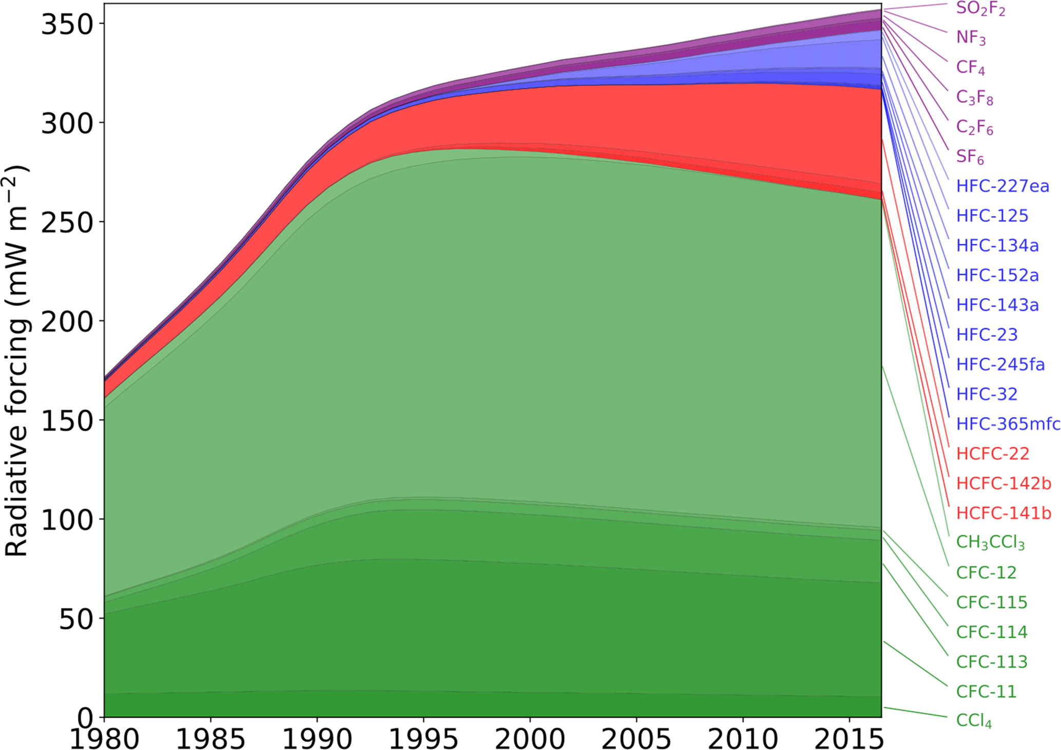
Figure 6Global radiative forcing due to long-lived SGHGs derived from AGAGE observations from 1980 to 2017 (update of Rigby et al., 2014).
AGAGE measures all of the significant SGHGs and Fig. 6 show global radiative forcing by each of these gases based on observations (Rigby et al., 2014, extended to 2017). CO2-equivalent emissions using 100-year GWPs have been derived from AGAGE observations for HFCs and PFCs plus SF6, NF3, and SO2F2 and compared to reported emissions from Annex-1 countries that are signatories to the United Nations Framework Convention on Climate Change (UNFCCC). Unreported emissions from non-Annex-1 countries (i.e., AGAGE-derived total emissions minus Annex-1 reported emissions) have been rapidly increasing since 1990 for both these classes of SGHGs and are now 35 % more than Annex-1 for the HFCs and 600 % more for the PFCs plus SF6. The mole fractions and derived emissions of AGAGE-measured heavy HFCs have all been increasing rapidly since the early 2000s for HFC-365mfc and HFC-245fa and since 1995 for HFC-227ea and HFC-236fa (Vollmer et al., 2011).
4.5 Trends in total radiative forcing
By adding the radiative forcing (W m−2) of the Montreal Protocol, Kyoto Protocol, and recent unregulated synthetic greenhouse gases, the overall radiative forcing due to all long-lived substances is obtained. Figure 7 shows that radiative forcing by CO2 still dominates, and the percentage of the total forcing due to the non-CO2 AGAGE greenhouse gases is slowly decreasing, reaching ∼ 36 % by the end of 2016. However, the emissions, mole fractions, and absolute radiative forcing of non-CO2 gases continue to rise.
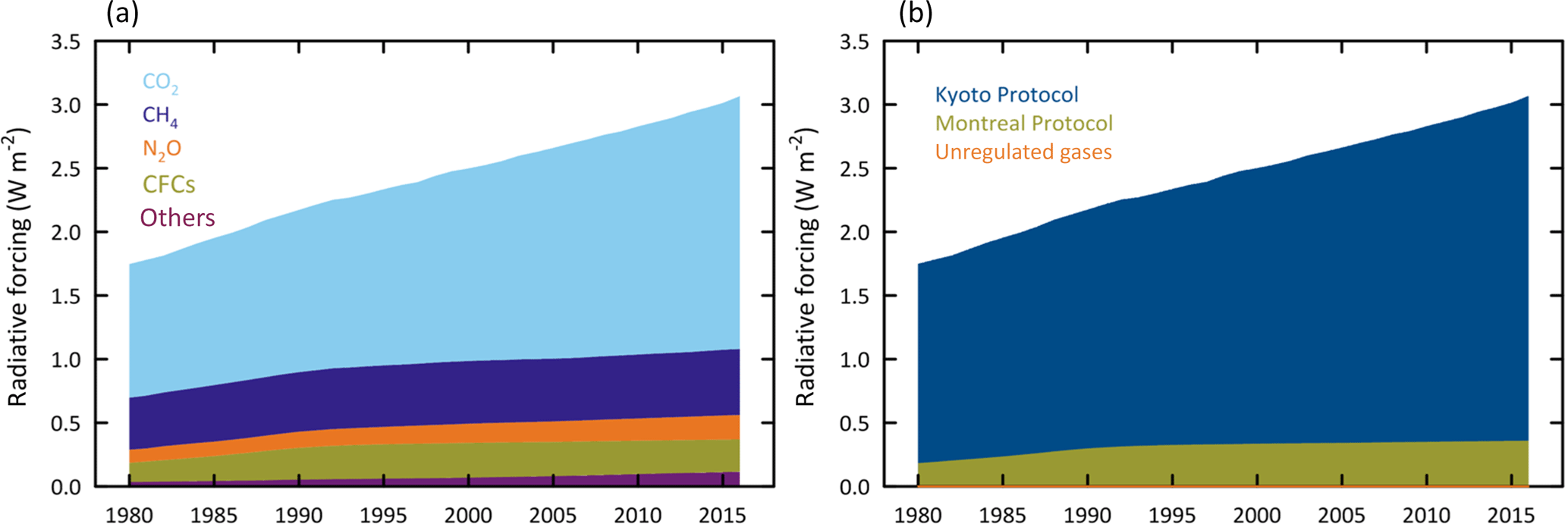
Figure 7Global total radiative forcing due to long-lived greenhouse gases derived from NOAA-GMD measurements for CO2 and AGAGE observations for all others (a). Also shown are the contributions from the gases in the Kyoto and Montreal Protocol and those not regulated by either protocol (b).
4.6 Determination of OH concentrations using models and multiple species
The hydroxyl free radical is the major oxidizing chemical in the atmosphere, destroying about 3.7 petagrams of trace gases each year, including many gases involved in ozone depletion, the greenhouse effect, and urban air pollution. The large-scale concentrations and long-term trends in OH can in principle be measured indirectly using global measurements of trace gases whose emissions are well known and whose primary sink is OH. The best trace gas for this purpose is the industrial chemical CH3CCl3. First, there are accurate long-term measurements of CH3CCl3 beginning in 1978 in the ALE/GAGE/AGAGE network (Prinn et al., 1983b, 2000, 2001, 2005, Rigby et al., 2008, 2013, 2017) and beginning in 1992 in the NOAA/CMDL network (Montzka et al., 2000, 2011). Second, CH3CCl3 has fairly simple end uses as a solvent, and voluntary chemical industry reports since 1970, along with the national reporting procedures under the Montreal Protocol in more recent years, have produced reasonably accurate emissions estimates for this chemical (McCulloch and Midgley, 2001). The use of CH3CCl3 for OH concentration and trend estimation has been extensive (Prinn et al., 1987, 1995, 2001, 2005; Spivakovsky et al., 2000; Montzka et al., 2000, 2011b; Krol and Lelieveld, 2003; Bousquet et al., 2005). Generally, interannual variability in OH inferred from CH3CCl3 inversions is larger than those calculated in atmospheric photochemical models (e.g., Montzka et al., 2011b), and the reasons are currently unresolved. Other gases that are useful OH indicators include 14CO, which is produced primarily by cosmic rays (Manning et al., 2005). Using HCFC-22 measurements for estimating the average OH yields similar results to those derived from CH3CCl3 but with less accuracy (Miller et al., 1998; Fortems-Cheiney et al., 2013). The industrial gases HFC-134a, HCFC-141b, and HCFC-142b are potentially useful OH estimators but the accuracy of their emission estimates needs improvement (Huang and Prinn, 2002; Fortems-Cheiney et al., 2015). At the present time, to augment CH3CCl3, the potential OH estimation species (the major tropospheric sink is reaction with OH, and industrial emissions estimations are relatively good) are HFC-134a, HCFC-141b, HCFC-142b, and possibly some of the newly introduced HFCs (Liang et al., 2017).
AGAGE data (Fig. 8) show that CH3CCl3 levels and latitudinal gradient rose steadily from 1978 to reach a maximum in 1992 and have both since rapidly decreased as the Montreal Protocol drove emissions to near zero. In 2010 the levels were about 3 % of those when AGAGE measurements began in 1978. Analysis of these observations shows that global average OH levels vary from year to year only occasionally significantly, but exhibit no significant long-term trend (Prinn et al., 2001, 2005; Rigby et al., 2008, 2013, 2017, latter updated in Fig. 8). This analysis includes the effects of observationally derived corrections to emissions and model and measurement errors. The 1997–1999 OH minimum coincides with, and is perhaps caused by, major global wildfires and an intense El Niño event at that time. Recent CH3CCl3 inversions have proposed a role for a rise and fall in OH in the pause and renewed growth of atmospheric methane (McNorton et al., 2016; Rigby et al., 2017; Turner et al., 2017). However, these trends were not found to be statistically significant when all uncertainties were considered.
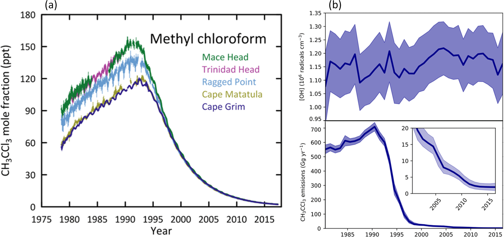
Figure 8CH3CCl3 monthly mean mole fractions and 1σ standard deviations at selected AGAGE stations (a). Global 12-month running mean OH concentrations and CH3CCl3 emissions from the AGAGE data and AGAGE 2-D model inversion. Shaded areas give 1σ uncertainty (b) (Rigby et al., 2017; updated here).
4.7 AGAGE emissions estimates for all gases
A major objective of all the AGAGE GC-MD and GC-MS measurements is to produce estimates of global emissions, spatial distributions of emissions, and their trends. These results are given in a large number of AGAGE publications (see Sects. 4.9, 5, and the references) and a selected few will be reviewed here. These AGAGE estimates are then critically compared against estimates provided from manufacturing and sales information for anthropogenic chemicals and from independently derived estimates for natural emissions to improve emission estimates and models. The error bars on the inferred emissions of trace gases in Fig. 4 reflect the uncertainties in the estimates that are generally dominated by uncertainties in point measurement to grid box model extrapolations and in chemical transport models including the species lifetimes.
AGAGE data have helped resolve some important emission controversies. For example, CH3CCl3 is an ozone-depleting industrial solvent whose phase-out was introduced under the Montreal Protocol. However, as the phase-out continued the reported emissions appeared too low to explain observations, and unreported European emissions were claimed to be a major cause (Krol et al., 2003). Long-term high-frequency AGAGE data from Mace Head and Jungfraujoch were used to infer European CH3CCl3 emissions to better quantify these unreported emissions. European emission estimates declined from about 60 gigagrams per year in the mid-1990s to 0.3–3.4 gigagrams per year in 2000–2003 based on Mace Head and Jungfraujoch data, respectively. These European CH3CCl3 emission estimates were higher than calculated from consumption data, but were considerably lower than those derived for 2000 in the Krol et al. (2003) study (Reimann et al., 2005). AGAGE is unusual amongst global networks in that 30 % of its in situ Medusa GC-MS observational capacity is located in the tropics (Fig. 1). A consistent feature that has emerged from AGAGE research over the period 2011–2015 is the importance of the tropics as the major source region for several important trace gases of biological origin: methane, nitrous oxide, methyl chloride, and hydrogen. Rigby et al. (2008) showed that the 2007 increase in methane growth rate in the atmosphere was likely due to a combination of emissions from unusually warm boreal summers and unusually wet tropical regions. Xiao et al. (2010a) confirmed the major role (> 50 %) that tropical plants play as a source of methyl chloride, the largest natural source of chlorine for the stratosphere. Huang et al. (2008) showed the importance of tropical regions and the Indian subcontinent as major source regions (> 80 %) for nitrous oxide, and Xiao et al. (2007) demonstrated the importance of tropical regions as the major (70 %) source (oxidation of formaldehyde, biomass burning) and major (70 %) sink (surface uptake, oxidation by OH) region for atmospheric hydrogen.
4.8 Emission estimates from multiple networks and measurement platforms and alternative models
In the last decade there has been a distinct move toward trace gas emission estimations using measurements from multiple networks and platforms. A number of the multi-network studies also applied alternative models and inverse methods to those used in AGAGE (Sect. 3.4–3.7). The methane flux estimations by Chen and Prinn (2006) merged for the first time the high-frequency AGAGE data with the low-frequency NOAA/ESRL/GMD, CSIRO, Environment Canada, NIES, and Japan Meteorological Agency flask data. The intercalibration process proved to be very important to this merger and showed that when done correctly the merger increases the precision and accuracy of the fluxes significantly. A formal intercalibration exercise began between the AGAGE, NOAA/ESRL/GMD, and other networks that used intercomparisons between instruments and flask sampling at the same station led by Paul B. Krummel (CSIRO) and intercomparisons of tanks of compressed air circulated among laboratories (IHALACE, Hall et al., 2014). This has enabled a significant number of subsequent studies that involve merging AGAGE data with data from other surface networks and platforms (towers, aircraft, satellites). AGAGE data and GMD (flask, tower, aircraft) data were used to obtain sources and/or sinks of SF6 (Rigby et al., 2010), CFCs and CH3CCl3 (Rigby et al., 2013), HCFC-22 (Saikawa et al., 2012, 2014b), CFCs and N2O (Simmonds et al., 2013), N2O (Nevison et al., 2011; Thompson et al., 2013, 2014a, b, c), methane (Thompson et al., 2015), CH3Cl (Xiao et al., 2010a), and CCl4 (Xiao et al., 2010b). HIPPO aircraft, AGAGE, and ESRL data were used for seasonal emissions of HCFC-22 and HFC-134a (Xiang et al., 2014) and for OH estimation (Patra et al., 2014). Kirschke et al. (2013) used AGAGE, GMD flask, CSIRO flask, and UCI aircraft data for estimating methane emissions. MIPAS, AGAGE, and GMD data were used by Chirkov et al. (2016) for estimating HCFC-22 emissions, and AGAGE and GMD data were used for estimating CCl4 emissions (Chipperfield et al., 2016); GOSAT, AGAGE, and GMD data were used for estimating regional methane emissions (Fraser et al., 2013). Saunoir et al. (2016, 2017) used multi-network data and alternative models to elucidate the 2000–2012 methane budget and its multiyear variability. Finally, Rigby et al. (2017) used AGAGE and GMD data for the estimation of OH concentrations and CH4 emissions, and Ganesan et al. (2017) used GOSAT satellite, CARIBIC aircraft, and AGAGE-calibrated surface measurements to estimate Indian subcontinent CH4 emissions.
4.9 AGAGE publications
The central accomplishments of the ALE/GAGE/AGAGE program are documented in several hundred journal publications and theses. A full list of all ALE/GAGE/AGAGE publications in the 1983–2017 time period supported by and/or collaborating with AGAGE is available on the official AGAGE website: http://agage.mit.edu (last access: 21 May 2018); click on RESEARCH, then AGAGE PUBLICATIONS, then AGAGE ACCOMPLISHMENTS (for abstracts). For AGAGE publications with “et al.”, the complete author list can be seen by clicking on the paper title in orange text. ALE/GAGE/AGAGE measurements and derived lifetimes, OH concentrations, and emissions are of considerable policy significance and are widely used in international and national ozone layer and climate assessments. AGAGE team members have specifically contributed as authors to almost all of the major international assessments under the IPCC and WMO.
After calibration, validation, and conversion to a prescribed format, AGAGE data for nine stations (Ny-Ålesund, Mace Head, Trinidad Head, Jungfraujoch, Monte Cimone, Gosan (monthly means), Ragged Point, Cape Matatula, Cape Grim) are made available on the AGAGE public website (http://agage.mit.edu/data, last access: 21 May 2018). The data from the newest station, Mt. Mugogo, will be added to this site once internally validated and the first data are published in peer-reviewed journals. Data from Shangdianzi (Bo Yao; yaob@cma.gov.cn), Hateruma, and Cape Ochiishi (Takuya Saito; saito.takuya@nies.go.jp) can be obtained by contacting the indicated station scientists. Data files for individual measurements and for monthly mean summaries are updated at approximately 6-month intervals, following the semiannual meetings of the international AGAGE team. Data considered a pollution event or a local sink event are flagged. Monthly means and standard deviations of the data with and without these events are included.
The data are currently available through March 2017.
Data files for measurements are updated and archived at approximately 6-month intervals, following quality-control reviews before and at the semiannual meetings of the AGAGE team. For scientific credibility, we do not submit data on new gases until at least one peer-reviewed AGAGE paper on that new gas has appeared. Because AGAGE is an international research (not operational) endeavor and because data validation for some gases can sometimes take longer than others, there is not a strict timetable between data acquisition and data submission, but generally we aim to archive data 12–18 months after acquisition.
The data on the AGAGE website are also made available on the US Department of Energy (DOE) Carbon Dioxide Information Analysis Center (CDIAC) website for public access (http://cdiac.ess-dive.lbl.gov/ndps/alegage.html, last access: 21 May 2018; Prinn et al., 2018). Note that data previously stored at the CDIAC archive are being transitioned to the new DOE ESS-DIVE archive. The above website will continue to provide access to the CDIAC data during the transition. Please contact ess-dive-support@lbl.gov for further information on the transition. CDIAC also passes on these data to the World Data Center for Greenhouse Gases (WDCGG) in Japan (http://ds.data.jma.go.jp/gmd/wdcgg/, last access: 21 May 2018). The AGAGE data in the WDCGG data center, however, are further processed by WDCGG staff and are converted to a different format from that used by the CDIAC and AGAGE websites. Thus, we do not recommend this site as a primary source of AGAGE data.
The authors declare that they have no conflict of interest.
We express our deep appreciation of the exceptional multi-decadal
contributions of the late Prof. Derek M. Cunnold (GaTech) to all aspects of
the AGAGE program, especially in the area of inverse modeling for source and
sink estimation. We note with sadness the significant contributions to AGAGE
of the late Laurie Porter (Bureau of Meteorology, Cape Grim) and the late Dr.
Brian Greally (U. Bristol, Mace Head). We specifically acknowledge the
cooperation and efforts of the following on-site station operators: Gerry
Spain, Mace Head, Ireland; Randy Dickau, Trinidad Head, California; Peter
Sealy, Ragged Point, Barbados; NOAA officers in charge, Cape Matatula,
American Samoa; Sam Cleland, Jeremy Ward, and Nigel Somerville, Cape Grim,
Tasmania; the Käser,
Fischer, Otz, Seiler, and Hemund families, Jungfraujoch, Switzerland; Kieran
Stanley, Ridge Hill, Bilsdale, and Heathfield, UK; and Stephen Humphery and
Andy McDonald, Tacolneston, UK. Nada Derek is gratefully thanked for her
assistance with the preparation of figures in this paper and her long-term
support of the AGAGE activities. We thank Kat Potter and Arnico Panday, who
played significant roles in establishing the Mt. Mugogo, Rwanda station.
Finally we thank Jim Butler, Ed Dlugokencky, Jim Elkins, Brad Hall, and Steve
Montzka of NOAA-ESRL-GMD for their valuable cooperation over many years in
measurement intercomparisons and other scientific activities. The operation
of the Mace Head, Trinidad Head, Barbados, American Samoa, and Tasmania AGAGE
stations and the MIT theory and inverse modeling and SIO calibration
activities are supported by the National Aeronautics and Space Administration
(NASA, USA; grants NAG5-12669, NNX07AE89G, NNX11AF17G, and NNX16AC98G to MIT;
grants NAG5-4023, NNX07AE87G, NNX07AF09G, NNX11AF15G, and NNX11AF16G to SIO).
Additional support comes from the following: the UK Department for Business,
Energy and Industrial Strategy (BEIS, UK; formerly the Department of
Business, Energy, Industry and Strategy) contract GA01103 to the University
of Bristol and the UK Met Office for Mace Head and the UK DECC tall tower
Network; the National Oceanic and Atmospheric Administration (NOAA, USA)
contract RA133R15CN0008 to the University of Bristol for Barbados; NOAA for
the building operations of the American Samoa station; and the Commonwealth
Scientific and Industrial Research Organisation (CSIRO, Australia), the
Bureau of Meteorology (Australia), the Department of the Environment and
Energy (DoEE, Australia), and Refrigerant Reclaim Australia for Cape Grim.
Anita Ganesan and Matt Rigby are supported by NERC. The Hateruma and Cape
Ochiishi stations are supported fully by the Ministry of Environment of Japan
and NIES. Observations at the Jungfraujoch are supported by the Swiss Federal
Office for the Environment (FOEN) within the project HALCLIM, by ICOS-CH
(Integrated Carbon Observation System Research Infrastructure), and by the
International Foundation High Altitude Research Stations for Jungfraujoch and
Gornergrat (HFSJG). Operations at Zeppelin, Ny-Ålesund are funded by the
Norwegian Environment Agency. Monte Cimone research is supported by the
Italian National Research Council (CNR) under the NEXDATA project. Sunyoung
Park (and the Gosan AGAGE station) is supported by the Basic Science Research
Program through the National Research Foundation of Korea (NRF) funded by the
Ministry of Education (no. NRF-2016R1A2B2010663). The Shangdianzi AGAGE
station is fully supported by the Chinese Meteorological Administration.
Funding for the instruments at the new AGAGE Mt. Mugogo station comes from
the MIT Alumni Donors to the Rwanda-MIT Climate Observatory Project and the
MIT Center for Global Change Science (CGCS). Funding for the infrastructure
and operations comes from the Ministry of Education of Rwanda. Finally,
development costs for the MIT high-end 3-D models and inverse techniques used
in the theoretical analysis are supported significantly by grants from other
federal agencies and by the sponsors of the MIT CGCS and Joint Program on the
Science and Policy of Global Change.
Edited by: Vinayak Sinha
Reviewed by: two anonymous referees
Allan, D. W.: Statistics of atomic frequency standards, P. IEEE, 54, 221–230, https://doi.org/10.1109/PROC.1966.4634, 1966.
Arnold, T., Mühle, J., Salameh, P. K., Harth, C. M., Ivy, D. J., and Weiss, R. F.: Automated Measurement of Nitrogen Trifluoride in Ambient Air, Anal. Chem., 84, 4798–4804, https://doi.org/10.1021/ac300373e, 2012.
Arnold, T., Harth, C. M., Mühle, J., Manning, A. J., Salameh, P. K., Kim, J., Ivy, D. J., Steele, L. P., Petrenko, V. V., Severinghaus, J. P., Baggenstos, D., and Weiss, R. F.: Nitrogen trifluoride global emissions estimated from updated atmospheric measurements, P. Natl. Acad. Sci. USA, 110, 2029–2034, https://doi.org/10.1073/pnas.1212346110, 2013.
Arnold, T., Ivy, D. J., Harth, C. M., Vollmer, M. K., Mühle, J., Salameh, P. K., Steele, L. P., Krummel, P. B., Wang, J., Young, D., Lunder, C. R., Hermansen, O., Rhee, T. S., Kim, J., Reimann, S., O'Doherty, S., Fraser, P. J., Simmonds, P. G., Prinn, R. G., and Weiss, R. F.: HFC-43-10mee atmospheric abundances and global emission estimates, Geophys. Res. Lett., 41, 2228–2235, https://doi.org/10.1002/2013GL059143, 2014.
Bosilovich, M. G., Chen, J., Robertson, F. R., and Adler, R. F.: Evaluation of Global Precipitation in Reanalyses, J. Appl. Meteorol. Clim., 47, 2279–2299, 2008.
Bousquet, P., Hauglustaine, D. A., Peylin, P., Carouge, C., and Ciais, P.: Two decades of OH variability as inferred by an inversion of atmospheric transport and chemistry of methyl chloroform, Atmos. Chem. Phys., 5, 2635–2656, https://doi.org/10.5194/acp-5-2635-2005, 2005.
Butler, J. H., Yvon-Lewis, S. A., Lobert, J. M., King, D. B., Montzka, S. A., Bullister, J. L., Koropalov, V., Elkins, J. W., Hall, B. D., Hu, L., and Liu, Y.: A comprehensive estimate for loss of atmospheric carbon tetrachloride (CCl+4) to the ocean, Atmos. Chem. Phys., 16, 10899–10910, https://doi.org/10.5194/acp-16-10899-2016, 2016.
Carpenter, L. J., Reimann, S., Burkholder, J. B., Clerbaux, C., Hall, B. D., Hossaini, R., Laube, J. C., Yvon-Lewis, S. A., Blake, D. R., Dorf, M., Dutton, G. S., Fraser, P. J., Froidevaux, L., Hendrick, F., Hu, J., Jones, A., Krummel, P. B., Kuijpers, L. J. M., Kurylo, M. J., Liang, Q., Mahieu, E., Mühle, J., O'Doherty, S., Ohnishi, K., Orkin, V. L., Pfeilsticker, K., Rigby, M., Simpson, I. J., Yokouchi, Y., Engel, A., and Montzka, S. A.: Update on Ozone-Depleting Substances (ODSs) and Other Gases of Interest to the Montreal Protocol (Chapter 1), in: Scientific Assessment of Ozone Depletion: 2014, Global Ozone Research and Monitoring Project-Report No. 55, World Meteorological Organization, Geneva, Switzerland, 2014.
Chen, Y.-H. and Prinn, R. G.: Atmospheric modeling of high-frequency methane observations: Importance of interannually varying transport, J. Geophys. Res., 110, D10303, https://doi.org/10.1029/2004JD005542, 2005.
Chen, Y.-H. and Prinn, R. G.: Estimation of atmospheric methane emissions between 1996–2001 using a 3D global chemical transport model, J. Geophys. Res., 111, D10307, https://doi.org/10.1029/2005JD006058, 2006.
Chipperfield, M. P., Liang, Q., Rigby, M., Hossaini, R., Montzka, S. A., Dhomse, S., Feng, W., Prinn, R. G., Weiss, R. F., Harth, C. M., Salameh, P. K., Mühle, J., O'Doherty, S., Young, D., Simmonds, P. G., Krummel, P. B., Fraser, P. J., Steele, L. P., Happell, J. D., Rhew, R. C., Butler, J., Yvon-Lewis, S. A., Hall, B., Nance, D., Moore, F., Miller, B. R., Elkins, J. W., Harrison, J. J., Boone, C. D., Atlas, E. L., and Mahieu, E.: Model sensitivity studies of the decrease in atmospheric carbon tetrachloride, Atmos. Chem. Phys., 16, 15741–15754, https://doi.org/10.5194/acp-16-15741-2016, 2016.
Chirkov, M., Stiller, G. P., Laeng, A., Kellmann, S., von Clarmann, T., Boone, C. D., Elkins, J. W., Engel, A., Glatthor, N., Grabowski, U., Harth, C. M., Kiefer, M., Kolonjari, F., Krummel, P. B., Linden, A., Lunder, C. R., Miller, B. R., Montzka, S. A., Mühle, J., O'Doherty, S., Orphal, J., Prinn, R. G., Toon, G., Vollmer, M. K., Walker, K. A., Weiss, R. F., Wiegele, A., and Young, D.: Global HCFC-22 measurements with MIPAS: retrieval, validation, global distribution and its evolution over 2005–2012, Atmos. Chem. Phys., 16, 3345–3368, https://doi.org/10.5194/acp-16-3345-2016, 2016.
Cox, M. L., Sturrock, G. A., Fraser, P. J., Siems, S. T., Krummel, P. B., and O'Doherty, S.: Regional sources of methyl chloride, chloroform and dichloromethane identified from AGAGE observations at Cape Grim, Tasmania, 1998–2000, J. Atmos. Chem., 45, 79–99, 2003.
Cunnold, D. M., Fraser, P. J., Weiss, R. F., Prinn, R. G., Simmonds, P. G., Miller, B. R., Alyea, F. N., and Crawford, A. J.: Global trends and annual releases of CCl3F and CCl2F2 estimated from ALE/GAGE and other measurements from July 1978 to June 1991, J. Geophys. Res., 99, 1107–1126, 1994.
Cunnold, D. M., Steele, L. P., Fraser, P. J., Simmonds, P. G., Prinn, R. G., Weiss, R. F., Porter, L. W., Langenfelds, R. L., Krummel, P. B., Wang, H. J., Emmons, L., Tie, X. X., and Dlugokencky, E. J.: In-Situ measurements of atmospheric methane at GAGE/AGAGE sites during 1985–1999 and resulting source inferences, J. Geophys. Res., 107, ACH 20-1–ACH 20-18, https://doi.org/10.1029/2001JD001226, 2002.
De Mazière, M., Thompson, A. M., Kurylo, M. J., Wild, J. D., Bernhard, G., Blumenstock, T., Braathen, G. O., Hannigan, J. W., Lambert, J.-C., Leblanc, T., McGee, T. J., Nedoluha, G., Petropavlovskikh, I., Seckmeyer, G., Simon, P. C., Steinbrecht, W., and Strahan, S. E.: The Network for the Detection of Atmospheric Composition Change (NDACC): history, status and perspectives, Atmos. Chem. Phys., 18, 4935–4964, https://doi.org/10.5194/acp-18-4935-2018, 2018.
Derwent, R. G, Simmonds, P. G., Greally, B. R., O'Doherty, S., McCulloch, A., Manning, A., Reimann, S., Folini, D., and Vollmer, M. K.: The phase-in and phase-out of European emissions of HCFC-141b and HCFC-142b under the Montreal Protocol: Evidence from observations at Mace Head, Ireland from 1994–2004, Atmos. Environ., 41, 757–767, 2007.
Derwent, R. G., Simmonds, P. G., O'Doherty, S., Grant, A., Young, D., Cooke, M. C., Manning, A. J., Utembe, S. R., Jenkin, M. E., and Shallcross, D. E.: Seasonal cycles in short-lived hydrocarbons in baseline air masses arriving at Mace Head, Ireland, Atmos. Environ., 62, 89–96, https://doi.org/10.1016/j.atmosenv.2012.08.023, 2012.
Draxler, R. D. and Hess, G. D.: Description of the HYSPLIT-4 modelling system, NOAA Tech. Memo. ERL ARL-224, 24 pp., Air Resour. Lab., Silver Spring, MD, 1997.
Dunse, B., Steele, P., Wilson, S., Fraser, P., and Krummel, P.: Trace gas emissions from Melbourne Australia, based on AGAGE observations at Cape Grim, Tasmania, 1995–2000, Atmos. Environ., 39, 6334–6344, 2005.
Elkins, J. W., Butler, J. H., Hall, B., Montzka, S. A., and Moore, F. L.: Halocarbon and Other Trace Gases Group/Global Monitoring Division/Earth Systems Research Laboratory (NOAA/ESRL) website: available atg: http://www.esrl.noaa.gov/gmd/, Boulder, CO, updated data available on anonymous ftp site at: http://www.esrl.noaa.gov/gmd/dv/ftpdata.html (last access: 21 May 2018), 2015.
Enting, I. G.: Inverse Problems in Atmospheric Constituent Transport, Cambridge University Press, Cambridge CB2 2RU, UK, 2002.
Emmons, L. K., Walters, S., Hess, P. G., Lamarque, J.-F., Pfister, G. G., Fillmore, D., Granier, C., Guenther, A., Kinnison, D., Laepple, T., Orlando, J., Tie, X., Tyndall, G., Wiedinmyer, C., Baughcum, S. L., and Kloster, S.: Description and evaluation of the Model for Ozone and Related chemical Tracers, version 4 (MOZART-4), Geosci. Model Dev., 3, 43–67, https://doi.org/10.5194/gmd-3-43-2010, 2010.
Eyer, S., Tuzson, B., Popa, M. E., van der Veen, C., Röckmann, T., Rothe, M., Brand, W. A., Fisher, R., Lowry, D., Nisbet, E. G., Brennwald, M. S., Harris, E., Zellweger, C., Emmenegger, L., Fischer, H., and Mohn, J.: Real-time analysis of δ13C- and δD−CH4 in ambient air with laser spectroscopy: method development and first intercomparison results, Atmos. Meas. Tech., 9, 263–280, https://doi.org/10.5194/amt-9-263-2016, 2016.
Fang, X., Thompson, R. L., Saito, T., Yokouchi, Y., Kim, J., Li, S., Kim, K. R., Park, S., Graziosi, F., and Stohl, A.: Sulfur hexafluoride (SF6) emissions in East Asia determined by inverse modeling, Atmos. Chem. Phys., 14, 4779–4791, https://doi.org/10.5194/acp-14-4779-2014, 2014.
Fang, X., Stohl, A., Yokouchi, Y., Kim, J., Li, S., Saito, T., Park, S., and Hu, J.: Multiannual Top-Down Estimate of HFC-23 Emissions in East Asia, Environ. Sci. Technol., 49, 4345–4353, https://doi.org/10.1021/es505669j, 2015.
Forster, P., Ramaswamy, V., Artaxo, P., Berntsen, T., Betts, R., Fahey, D., Haywood, J., Lean, J., Lowe, D., Myhre, G., Nganga, J., Prinn, R., Raga, G., Schulz, M., Van Dorland, R.: Changes in Atmospheric Constituents and in Radiative Forcing, in: Climate Change 2007: The Physical Science Basis. Contribution of Working Group I to the Fourth Assessment Report of the Intergovernmental Panel on Climate Change, edited by: Solomon, S., Qin, S., Manning, M., Chen, Z., Marquis, M., Averyt, K., Tignor, M., and Miller, H.: Cambridge University Press, Cambridge, UK and New York, USA, chap. 2, 129–234, 2007.
Fortems-Cheiney, A., Chevallier, F., Saunois, M., Pison, I., Bousquest, P., Cressot, C., Wang, R. H. J., Yokouchi, Y., and Artuso, F.: HCFC-22 emissions at global and regional scales between 1995 and 2010: Trends and variability. J. Geophys. Res.-Atmos., 118, 7379–7388, 2013.
Fortems-Cheiney, A., Saunois, M., Pison, I., Chevallier, F., Bousquet, P., Cressot, C., Montzka, S. A., Fraser, P. J., Vollmer, M. K., Simmonds, P. G., Young, D., O'Doherty, S., Weiss, R. F., Artuso, F., Barletta, B., Blake, D. R., Li, S., Lunder, C., Miller, B. R., Park, S., Prinn, R., Saito, T., Steele, L. P., and Yokouchi, Y.: Increase in HFC-134a emissions in response to the success of the Montreal Protocol, J. Geophys. Res.-Atmos., 120, 11728–11742, https://doi.org/10.1002/2015JD023741, 2015.
Fraser, A., Palmer, P. I., Feng, L., Boesch, H., Cogan, A., Parker, R., Dlugokencky, E. J., Fraser, P. J., Krummel, P. B., Langenfelds, R. L., O'Doherty, S., Prinn, R. G., Steele, L. P., van der Schoot, M., and Weiss, R. F.: Estimating regional methane surface fluxes: the relative importance of surface and GOSAT mole fraction measurements, Atmos. Chem. Phys., 13, 5697–5713, https://doi.org/10.5194/acp-13-5697-2013, 2013.
Fraser, P. J., Dunse, B. L., Manning, A. J., Walsh, S., Wang, R. H. J., Krummel, P. B., Steele, L. P., Porter, L. W., Allison, C., O'Doherty, S., Simmonds, P. G., Mühle, J., Weiss, R. F., and Prinn, R. G.: Australian carbon tetrachloride (CCl4) emissions in a global context, Environ. Chem., 11, 77–88, https://doi.org/10.1071/EN13171, 2014.
Fraser, P. J., Pearman, G. I., and Derek, N.: CSIRO non-carbon dioxide greenhouse gas research. Part 1: 1975–1990, Hist. Rec. Aust. Sci., 29, 1–13, https://doi.org/10.1071/HR17016, 2017.
Ganesan, A. L., Rigby, M., Zammit-Mangion, A., Manning, A. J., Prinn, R. G., Fraser, P. J., Harth, C. M., Kim, K.-R., Krummel, P. B., Li, S., Mühle, J., O'Doherty, S. J., Park, S., Salameh, P. K., Steele, L. P., and Weiss, R. F.: Characterization of uncertainties in atmospheric trace gas inversions using hierarchical Bayesian methods, Atmos. Chem. Phys., 14, 3855–3864, https://doi.org/10.5194/acp-14-3855-2014, 2014.
Ganesan, A. L., Manning, A. J., Grant, A., Young, D., Oram, D. E., Sturges, W. T., Moncrieff, J. B., and O'Doherty, S.: Quantifying methane and nitrous oxide emissions from the UK and Ireland using a national-scale monitoring network, Atmos. Chem. Phys., 15, 6393–6406, https://doi.org/10.5194/acp-15-6393-2015, 2015.
Ganesan, A. L., Rigby, M., Lunt, M. F., Parker, R. J., Boesch, H., Goulding, N., Umezawa, T., Zahn, A., Chatterjee, A., Prinn, R. G., Tiwari, Y. K., van der Schoot, M., and Krummel, P. B.: Atmospheric observations show accurate reporting and little growth in India's methane emissions, Nat. Commun., 8, 1–7, https://doi.org/10.1038/s41467-017-00994-7, 2017.
Grant, A., Yates, E. L., Simmonds, P. G., Derwent, R. G., Manning, A. J., Young, D., Shallcross, D. E., and O'Doherty, S.: A five year record of high-frequency in situ measurements of non-methane hydrocarbons at Mace Head, Ireland, Atmos. Meas. Tech., 4, 955–964, https://doi.org/10.5194/amt-4-955-2011, 2011.
Graziosi, F., Arduini, J., Furlani, F., Giostra, U., Kuijpers, L. J. M., Montzka, S. A., Miller, B. R., O'Doherty, S. J., Stohl, A., Bonasoni, P., and Maione, M.: European emissions of HCFC-22 based on eleven years of high frequency atmospheric measurements and a Bayesian inversion method, Atmos. Environ., 112, 196–207, https://doi.org/10.1016/j.atmosenv.2015.04.042, 2015.
Graziosi, F., Arduini, J., Bonasoni, P., Furlani, F., Giostra, U., Manning, A. J., McCulloch, A., O'Doherty, S., Simmonds, P. G., Reimann, S., Vollmer, M. K., and Maione, M.: Emissions of carbon tetrachloride from Europe, Atmos. Chem. Phys., 16, 12849–12859, https://doi.org/10.5194/acp-16-12849-2016, 2016.
Graziosi, F., Arduini, J., Furlani, F., Giostra, U., Cristofanelli, P., Fang, X., Hermanssen, O., Lunder, C., Maenhout, G., O'Doherty, S., Reimann, S., Schmidbauer, N., Vollmer, M. K., Young, D., and Maione, M.: European emissions of the powerful greenhouse gases hydrofluorocarbons inferred from atmospheric measurements and their comparison with annual national reports to UNFCCC, Atmos. Environ., 158, 85–97, 2017.
Hall, B. D., Engel, A., Mühle, J., Elkins, J. W., Artuso, F., Atlas, E., Aydin, M., Blake, D., Brunke, E.-G., Chiavarini, S., Fraser, P. J., Happell, J., Krummel, P. B., Levin, I., Loewenstein, M., Maione, M., Montzka, S. A., O'Doherty, S., Reimann, S., Rhoderick, G., Saltzman, E. S., Scheel, H. E., Steele, L. P., Vollmer, M. K., Weiss, R. F., Worthy, D., and Yokouchi, Y.: Results from the International Halocarbons in Air Comparison Experiment (IHALACE), Atmos. Meas. Tech., 7, 469–490, https://doi.org/10.5194/amt-7-469-2014, 2014.
Harris, E., Nelson, D. D., Olszewski, W., Zahniser, M., Potter, K. E., McManus, B. J., Whitehill, A., Prinn, R. G., and Ono, S.: Development of a Spectroscopic Technique for Continuous Online Monitoring of Oxygen and Site-Specific Nitrogen Isotopic Composition of Atmospheric Nitrous Oxide, Anal. Chem., 86, 1726–1734, https://doi.org/10.1021/ac403606u, 2013.
Hartley, D. E. and Prinn, R. G.: On the feasibility of determining surface emissions of trace gases using an inverse method in a three-dimensional chemical transport model, J. Geophys. Res., 98, 5183–5198, 1993.
Hartmann, D. L., Klein Tank, A. M. G., Rusticucci, M., Alexander, L. V., Brönnimann, S., Charabi, Y., Dentener, F. J., Dlugokencky, E. J., Easterling, D. R., Kaplan, A., Soden, B. J., Thorne, P. W., Wild, M., and Zhai, P. M.: Observations: Atmosphere and Surface, in: Climate Change 2013: The Physical Science Basis, Contribution of Working Group I to the Fifth Assessment Report of the Intergovernmental Panel on Climate Change, edited by: Stocker, T. F., Qin, D., Plattner, G.-K., Tignor, M., Allen, S. K., Boschung, J., Nauels, A., Xia, Y., Bex, V., and Midgley, P. M., Cambridge University Press, Cambridge, United Kingdom and New York, NY, USA, 2013.
Heil, J., Wolf, B., Brüggemann, N., Emmenegger, L., Tuzson, B., Vereecken, H., and Mohn, J.: Site-specific 15N isotopic signatures of aiotically produced N2O, Geochim. Cosmochim. Ac., 139, 72–82, https://doi.org/10.1016/j.gca.2014.04.037, 2014.
Huang, J. and Prinn, R. G.: Critical evaluation of emissions for potential new OH titrating gases, J. Geophys. Res., 107, 4784, https://doi.org/10.1029/2002JD002394, 2002.
Huang, J., Golombek, A., Prinn, R., Weiss, R., Fraser, P., Simmonds, P., Dlugokencky, E. J., Hall, B., Elkins, J., Steele, P., Langenfelds, R., Krummel, P., Dutton, G., and Porter, L.: Estimation of regional emissions of nitrous oxide from 1997 to 2005 using multinetwork measurements, a chemical transport model, and an inverse method, J. Geophys. Res., 113, D17313, https://doi.org/10.1029/2007JD009381, 2008.
Ivy, D. J., Arnold, T., Harth, C. M., Steele, L. P., Mühle, J., Rigby, M., Salameh, P. K., Leist, M., Krummel, P. B., Fraser, P. J., Weiss, R. F., and Prinn, R. G.: Atmospheric histories and growth trends of , Atmos. Chem. Phys., 12, 4313–4325, https://doi.org/10.5194/acp-12-4313-2012, 2012a.
Ivy, D. J., Rigby, M., Baasandorj, M., Burkholder, J. B., and Prinn, R. G.: Global emission estimates and radiative impact of and C8F18, Atmos. Chem. Phys., 12, 7635–7645, https://doi.org/10.5194/acp-12-7635-2012, 2012b.
Jones, A., Thomson, D., Hort, M., and Devenish, B.: The UK Met Office's next-generation atmospheric dispersion model, NAME III, Air Pollution Modeling and Its Applications Xvii, 17, 580–589, https://doi.org/10.1007/978-0-387-68854-1_62, 2007.
Kalnay, E., Kanamitsu, M., Kistler, R., Collins, W., Deaven, D., Gandin, L., Iredell, M., Saha, S., White, G., Woollen, J., Zhu, Y., Leetmaa, A., Reynolds, R., Chelliah, M., Ebisuzaki, W., Higgins, W., Janowiak, J., Mo, K. C., Ropelewski, C., Wang, J., Jenne, R., and Joseph, D.: The NCEP/NCAR 40-Year Reanalysis Project, B. Am. Meteorol. Soc., 77, 437–471, 1996.
Kaminski, T., Rayner, P. J., Heimann, M., and Enting, I. G.: On aggregation errors in atmospheric transport inversions, J. Geophys. Res., 106, 4703–4715, 2001.
Kasibhatla, P., Heimann, M., Rayner, P., Mahowald, N., Prinn, R. G., and Hartley, D. (Eds): Inverse Methods in Global Biogeochemical Cycles, Geophysical Monograph Series, Volume 114, American Geophysical Union, Washington DC, 324 pp., 2000.
Keller, C. A., Brunner, D., Henne, S., Vollmer, M. K., O'Doherty, S., and Reimann, S.: Evidence for under-reported Western European emissions of the potent greenhouse gas HFC-23, Geophys. Res. Lett., 38, L15808, https://doi.org/10.1029/2011GL047976, 2011.
Keller, C. A., Hill, M., Vollmer, M. K., Henne, S., Brunner, D., Reimann, S., O'Doherty, S., Arduini, J., Maione, M., Ferenczi, Z., Haszpra, L., Manning, A. J., and Peter, T.: European emissions of halogenated greenhouse gases inferred from atmospheric measurements, Environ. Sci. Technol., 46, 217–225, https://doi.org/10.1021/es202453j, 2012.
Kim, J., Li, S., Kim, K.-R., Stohl, A., Mühle, J., Kim, S.-K., Park, M.-K., Kang, D.-J., Lee, G., Harth, C. M., Salameh, P. K., and Weiss, R. F.: Regional atmospheric emissions determined from measurements at Jeju Island, Korea: Halogenated compounds from China, Geophys. Res. Lett., 37, L12801, https://doi.org/10.1029/2010gl043263, 2010.
Kim, J., Li, S., Mühle, J., Stohl, A., Kim, S.-K., Park, S.. Park, M.-K., Weiss, R. F., and Kim, K.-R.: Overview of the findings from measurements of halogenated compounds at Gosan (Jeju Island, Korea) quantifying emissions in East Asia, J. Integr. Environ. Sci., 9, Supplement 1, 71–80, https://doi.org/10.1080/1943815X.2012.696548, 2012.
K im, J., Fraser, P. J., Li, S., Mühle, J., Ganesan, A. L., Krummel, P. B., Steele, L. P., Park, S., Kim, S.-K., Park, M.-K., Arnold, T., Harth, C. M., Salameh, P. K., Prinn, R. G., Weiss, R. F., and Kim, K.-R.: Quantifying aluminum and semiconductor industry perfluorocarbon emissions from atmospheric measurements, Geophys. Res. Lett., 41, 4787–4794, https://doi.org/10.1002/2014GL059783, 2014.
Kirschke, S., Bousquet, P., Ciais, P., Marielle Saunois, M., Canadell, J. G., Dlugokencky, E. J., Bergamaschi, P., Bergmann, D., Blake, D. R., Bruhwiler, L., Cameron-Smith, P., Castaldi, S., Chevallier, F., Feng, L., Fraser, A., Fraser, P. J., Heimann, M., Hodson, E. L., Houweling, S., Josse, B., Krummel, P. B, Lamarque, J.-F., Langenfelds, R. L., Le Quéré, C., Naik, V., O'Doherty, S., Palmer, P. I., Pison, I., Plummer, D., Poulter, B., Prinn, R. G., Rigby, M., Ringeval, B., Santini, M., Schmidt, M., Shindell, D.T., Simpson, I. J., Spahni, R., Steele, L.P., Strode, S. A., Sudo, K., Szopa, S., van der Werf, G. R., Voulgarakis, A., van Weele, M., Weiss, R. F., Williams, J. E., and Zeng, G.: Three decades of global methane sources and sinks, Nat. Geosci., 6, 813–823, https://doi.org/10.1038/NGEO1955, 2013.
Kleiman, G. and Prinn, R. G.: Measurement and deduction of emissions of trichloroethene, tetrachloroethene and trichloromethane (chloroform) in the Northeastern U.S. and Southeastern Canada, J. Geophys. Res., 105, 28875–28893, 2000.
Krol, M. and Lelieveld, J.: Can the variability in tropospheric OH be deduced from measurements of 1,1,1-trichloroethane (methyl chloroform)?, J. Geophys. Res., 108, ACH16, https://doi.org/10.1029/2002JD002423, 2003.
Krol, M., Lelieveld, J., Oram, D. E., Sturrock, G. A., Penkett, S. A., Brenninkmeijer, C. A. M., Gros, V., Williams, J., and Scheeren, H. A.: Continuing emissions of methyl chloroform from Europe, Nature, 421, 131–135, 2003.
Lawrence, M. G., Crutzen, P. J., Rasch, P. J., Eaton, B. E., and Mahowald, N. M.: A model for studies of tropospheric photochemistry: description, global distributions and evaluation, J. Geophys. Res., 104, 26245–26277, 1999.
Li, J., Cunnold, D. M., Wang, H.-J., Weiss, R. F., Miller, B. R., Harth, C., Salameh, P., and Harris, J. M.: Halocarbon emissions estimated from Advanced Global Atmospheric Gases Experiment measured pollution events at Trinidad Head, California, J. Geophys. Res., 110, D14308, https://doi.org/10.1029/2004JD005739, 2005.
Li, S., Kim, J., Kim, K.-R., Mühle, J., Kim, S.-K., Park, M.-K., Stohl, A., Kang, D.-J., Arnold, T., Harth, C. M., Salameh, P. K., and Weiss, R.F.: Emissions of halogenated compounds in East Asia determined from measurements at Jeju Island, Korea, Environ. Sci. Technol., 45, 5668–5675, https://doi.org/10.1021/es104124k, 2011.
Li, S., Kim, J., Park, S., Kim, S.-K., Park, M.-K., Mühle, J., Lee, G., Lee, M., Jo, C. O., and Kim, K.-R.: Source Identification and Apportionment of Halogenated Compounds Observed at a Remote Site in East Asia, Environ. Sci. Technol., 48, 491–498, https://doi.org/10.1021/es402776w, 2014.
Liang, Q., Chipperfield, M. P., Fleming, E. L., Abraham, N. L., Braesicke, P., Burkholder, J. B., Daniel, J. S., Dhomse, S., Fraser, P. J., Hardiman, S. C., Jackman, C. H., Kinnison, D.E., Krummel, P. B., Montzka, S. A., Morgenstern, O., McCulloch, A., Mühle, J., Newman, P.A., Orkin, V. L., Pitari, G., Prinn, R. G., Rigby, M., Rozanov, E., Stenke, A., Tummon, F., Velders, G. J. M., Visioni, D., and Weiss, R. F.: Deriving global OH abundance and atmospheric lifetimes for long-lived gases: A search for CH3CCl3 alternatives, J. Geophys. Res.-Atmos., 122, 11914–11933, https://doi.org/10.1002/2017JD026926, 2017.
Locatelli, R., Bousquet, P., Chevallier, F., Fortems-Cheney, A., Szopa, S., Saunois, M., Agusti-Panareda, A., Bergmann, D., Bian, H., Cameron-Smith, P., Chipperfield, M. P., Gloor, E., Houweling, S., Kawa, S. R., Krol, M., Patra, P. K., Prinn, R. G., Rigby, M., Saito, R., and Wilson, C.: Impact of transport model errors on the global and regional methane emissions estimated by inverse modelling, Atmos. Chem. Phys., 13, 9917–9937, https://doi.org/10.5194/acp-13-9917-2013, 2013.
Loh, Z. M., Law, R. M., Haynes, K. D., Krummel, P. B., Steele, L. P., Fraser, P. J., Chambers, S. D., and Williams, A. G.: Simulations of atmospheric methane for Cape Grim, Tasmania, to constrain southeastern Australian methane emissions, Atmos. Chem. Phys., 15, 305–317, https://doi.org/10.5194/acp-15-305-2015, 2015.
Lo Vullo, E., Furlani, F., Arduini, J., Giostra, U., Cristofanelli, P., Williams, M. L., and Maione, M.: Non- Methane Volatile Organic Compounds in the Background Atmospheres of a Southern European Mountain Site (Mt. Cimone, Italy): Annual and Seasonal Variability, Aerosol Air Qual. Res., 16, 581–592, https://doi.org/10.4209/aaqr.2015.05.0364, 2016a.
Lo Vullo, E., Furlani, F., Arduini, J., Giostra, U., Graziosi, F., Cristofanelli, P., Williams, M. L., and Maione, M.: Anthropogenic non-methane volatile hydrocarbons at Mt. Cimone (2165 m a.s.l, Italy): Impact of sources and transport on atmospheric composition, Atmos. Environ., 140, 395–440, https://doi.org/10.1016/j.atmosenv.2016.05.060, 2016b.
Lunt, M. F., Rigby, M., Ganesan, A. L., Manning, A. J., Prinn, R. G., O'Doherty, S., Muhle, J., Harth, C. M., Salameh, P. K., Arnold, T., Weiss, R. F., Saito, T., Yokouchi, Y., Krummel, P. B., Steele, L. P., Fraser, P. J., Li, S., Park, S., Reimann, S., Vollmer, M. K., Lunder, C., Hermansen, O., Schmidbauer, N., Maione, M., Young, D., and Simmonds, P. G.: Reconciling reported and unreported HFC emissions with atmospheric observations, P. Natl. Acad. Sci. USA, 112, 5927–5931, https://doi.org/10.1073/pnas.1420247112, 2015.
Lunt, M. F., Rigby, M., Ganesan, A. L., and Manning, A. J.: Estimation of trace gas fluxes with objectively determined basis functions using reversible-jump Markov chain Monte Carlo, Geosci. Model Dev., 9, 3213–3229, https://doi.org/10.5194/gmd-9-3213-2016, 2016.
MacFarling-Meure, C., Etheridge, D., Trudinger, C., Steele, P., Langenfelds, R., van Ommen, T., Smith, A., and Elkins, J.: Law Dome CO2, CH4, and N2O ice core records extended to 2000 years BP, Geophys. Res. Lett., 33, L14810, https://doi.org/10.1029/2006GL026152, 2006.
Mahowald, N. M., Prinn, R. G., and Rasch, P. J.: Deducing CCl3F emissions using an inverse method and chemical transport models with assimilated winds, J. Geophys. Res., 102, 28153–28168, 1997.
Maione, M., Giostra, U., Arduini, J., Furlani, F., Graziosi, F., Lo Vullo, E., and Bonasoni, P.: Ten years of continuous observations of stratospheric ozone depleting gases at Monte Cimone (Italy) – Comments on the effectiveness of the Montreal Protocol from a regional perspective, Sci. Total Environ., 445–446, 155–164, 2013.
Maione, M., Graziosi, F., Arduini, J., Furlani, F., Giostra, U., Blake, D. R., Bonasoni, P., Fang, X., Montzka, S. A., O'Doherty, S. J., Reimann, S., Stohl, A., and Vollmer, M. K.: Estimates of European emissions of methyl chloroform using a Bayesian inversion method, Atmos. Chem. Phys., 14, 9755–9770, https://doi.org/10.5194/acp-14-9755-2014, 2014.
Manning, A., O'Doherty, S., Jones, A. R., Simmonds, P. G., and Derwent, R. G.: Estimating UK methane and nitrous oxide emissions from 1990 to 2007 using an inversion modeling approach, J. Geophys. Res., 116, D02305, https://doi.org/10.1029/2010JD014763, 2011.
Manning, M. R., Lowe, D. C., Moss, R. C., Bodeker, G. E., and Allan, W.: Short term variations in the oxidizing power of the atmosphere, Nature, 436, 1001–1004, 2005.
McCulloch, A. and Midgley, P.: The history of methyl chloroform emissions: 1951–2000, Atmos. Environ., 35, 5311–5319, 2001.
McNorton, J., Chipperfield, M. P., Gloor, M., Wilson, C., Feng, W., Hayman, G. D., Rigby, M., Krummel, P. B., O'Doherty, S., Prinn, R. G., Weiss, R. F., Young, D., Dlugokencky, E., and Montzka, S. A.: Role of OH variability in the stalling of the global atmospheric CH4 growth rate from 1999 to 2006, Atmos. Chem. Phys., 16, 7943–7956, https://doi.org/10.5194/acp-16-7943-2016, 2016.
Meinshausen, M., Vogel, E., Nauels, A., Lorbacher, K., Meinshausen, N., Etheridge, D. M., Fraser, P. J., Montzka, S. A., Rayner, P. J., Trudinger, C. M., Krummel, P. B., Beyerle, U., Canadell, J. G., Daniel, J. S., Enting, I. G., Law, R. M., Lunder, C. R., O'Doherty, S., Prinn, R. G., Reimann, S., Rubino, M., Velders, G. J. M., Vollmer, M. K., Wang, R. H. J., and Weiss, R.: Historical greenhouse gas concentrations for climate modelling (CMIP6), Geosci. Model Dev., 10, 2057–2116, https://doi.org/10.5194/gmd-10-2057-2017, 2017.
Meirink, J. F., Bergamaschi, P., and Krol, M. C.: Four-dimensional variational data assimilation for inverse modelling of atmospheric methane emissions: method and comparison with synthesis inversion, Atmos. Chem. Phys., 8, 6341–6353, https://doi.org/10.5194/acp-8-6341-2008, 2008.
Miller, B. R., Weiss, R. F., Prinn, R. G., Huang, J., and Fraser, P. J.: Atmospheric trend and lifetime of chlorodifluoromethane (HCFC-22) and the global tropospheric OH concentration, J. Geophys. Res., 103, 13237–13248, 1998.
Miller, B. R., Weiss, R. F., Salameh, P. K., Tanhua, T., Greally, B. R., Mühle, J., and Simmonds, P.: Medusa: a sample preconcentration and GC-MSD system for in situ measurements of atmospheric trace halocarbons, hydrocarbons and sulfur compounds, Anal. Chem., 80, 1536–1545, 2008.
Miller, B. R., Rigby, M., Kuijpers, L. J. M., Krummel, P. B., Steele, L. P., Leist, M., Fraser, P. J., McCulloch, A., Harth, C., Salameh, P., Mühle, J., Weiss, R. F., Prinn, R. G., Wang, R. H. J., O'Doherty, S., Greally, B. R., and Simmonds, P. G.: HFC-23 (CHF3) emission trend response to HCFC-22 (CHClF2) production and recent HFC-23 emission abatement measures, Atmos. Chem. Phys., 10, 7875–7890, https://doi.org/10.5194/acp-10-7875-2010, 2010.
Mohn, J., Guggenheim, C., Tuzson, B., Vollmer, M. K., Toyoda, S., Yoshida, N., and Emmenegger, L.: A liquid nitrogen-free preconcentration unit for measurements of ambient N2O isotopomers by QCLAS, Atmos. Meas. Tech., 3, 609–618, https://doi.org/10.5194/amt-3-609-2010, 2010.
Mohn, J., Wolf, B., Toyoda, S., Lin, C.-T., Liang, M.-C., Brüggemann, N., Wissel, H., Steiker, A. E., Dyckmans, J., Szwec, L., Ostrom, N. E., Casciotti, K. L., Forbes, M., Giesemann, A., Well, R., Doucett, R. R., Yarnes, C. T., Ridley, A. R., Kaiser, J., and Yoshida, N., Interlaboratory assessment of nitrous oxide isotopomer analysis by isotope ratio mass spectrometry and laser spectroscopy: current status and perspectives. Rapid Commun. Mass Spectrom., 28, 1995–2007, https://doi.org/10.1002/rcm.6982, 2014.
Montzka, S. A., Spivakovsky, C. M., Butler, J. H., Elkins, J. W., Lock, L. T., and Mondeel, D. J.: New observational constraints on atmospheric hydroxyl on global and hemispheric scales, Science, 288, 500–503, 2000.
Montzka, S. A., Reimann, S., Engel, A., Krüger, K., O'Doherty, S., Sturges, W. T., Blake, D., Dorf, M., Fraser, P., Froidevaux, L., Jucks, K., Kreher, K., Kurylo, M. J., Mellouki, A., Miller, J., Nielsen, O.-J., Orkin, V. L., Prinn, R. G., Rhew, R., Santee, M. L., Stohl, A., and Verdonik, D.: Ozone-Depleting Substances (ODSs) and Related Chemicals, Chapter 1, in: Scientific Assessment of Ozone Depletion: 2010, World Meteorological Organization, Geneva, Switzerland, 2011a.
Montzka, S., Krol, M., Dlugokencky, E., Hall, B., Jockel, P., and Lelieveld, J.: Small interannual variability of global atmospheric hydroxyl, Science, 331, 67–69, https://doi.org/10.1126/science.1197640, 2011b.
Montzka, S. A., Dutton, G. S., Yu, P., Ray, E., Portmann, R. W., Daniel, J. S., Kuijpers, L., Hall, B. D., Mondeel, D., Siso, C., Nance, D. J., Rigby, M., Manning, A. J., Hu, L., Moore, F., Miller, B. R., and Elkins, J. W.: A persistent and unexpected increase in global emissions of ozone-depleting CFC-11, Nature, 557, 413–417, https://doi.org/10.1038/s41586-018-0106-2, 2018, 2018.
Mühle, J., Huang, J., Weiss, R. F., Prinn, R. G., Miller, B. R., Salameh, P. K., Harth, C. M., Fraser, P. J., Porter, L. W., Greally, B. R., O'Doherty, S., Simmonds, P. G., Krummel, P. B., and Steele, L. P.: Sulfuryl Fluoride in the Global Atmosphere, J. Geophys. Res., 114, D05306, https://doi.org/10.1029/2008JD011162, 2009.
Mühle, J., Ganesan, A. L., Miller, B. R., Salameh, P. K., Harth, C. M., Greally, B. R., Rigby, M., Porter, L. W., Steele, L. P., Trudinger, C. M., Krummel, P. B., O'Doherty, S., Fraser, P. J., Simmonds, P. G., Prinn, R. G., and Weiss, R. F.: Perfluorocarbons in the global atmosphere: tetrafluoromethane, hexafluoroethane, and octafluoropropane, Atmos. Chem. Phys., 10, 5145–5164, https://doi.org/10.5194/acp-10-5145-2010, 2010.
Mulquiney, J. E., Taylor, J. A., Jakeman, A. J., Norton, J. P., and Prinn, R. G.: A new inverse method for trace gas flux estimation, 2. Application to tropospheric CFCl3 fluxes, J. Geophys. Res., 103, 1429–1442, 1998.
Nevison, C. D., Dlugokencky, E., Dutton, G., Elkins, J. W., Fraser, P., Hall, B., Krummel, P. B., Langenfelds, R. L., O'Doherty, S., Prinn, R. G., Steele, L. P., and Weiss, R. F.: Exploring causes of interannual variability in the seasonal cycles of tropospheric nitrous oxide, Atmos. Chem. Phys., 11, 3713–3730, https://doi.org/10.5194/acp-11-3713-2011, 2011.
Obersteiner, F., Bönisch, H., and Engel, A.: An automated gas chromatography time-of-flight mass spectrometry instrument for the quantitative analysis of halocarbons in air, Atmos. Meas. Tech., 9, 179–194, https://doi.org/10.5194/amt-9-179-2016, 2016.
O'Doherty, S., Simmonds, P., Cunnold, D., Wang, R. H. J., Sturrock, G. A., Fraser, P. J., Ryall, D., Derwent, R. G., Weiss, R. F., Salameh, P., Miller, B. R., and Prinn, R. G.: In Situ Chloroform Measurements at AGAGE Atmospheric Research Stations from 1994–1998, J. Geophys. Res., 106, 20429–20444, 2001.
O'Doherty, S., Cunnold, D. M., Manning, A., Miller, B. R., Wang, R. H., Krummel, P. B., Fraser, P. J., Simmonds, P. G., McCulloch, A., Weiss, R. F., Salameh, P. Porter, L. W., Prinn, R. G., Huang, J., Sturrock, G., Ryall, D., Derwent, R. G., and Montzka, S. A.: Rapid growth of hydrofluorocarbon 134a and hydrochlorofluorocarbons 141b, 142b, and 22 from Advanced Global Atmospheric Gases Experiment (AGAGE) observations at Cape Grim Tasmania, and Mace Head, Ireland, J. Geophys. Res.,109, D06310, https://doi.org/10.1029/2003JD004277, 2004.
O'Doherty, S., Cunnold, D. M., Miller, B. R., Mühle, J., McCulloch, A., Simmonds, P. G., Manning, A. J., Reimann, S., Vollmer, M. K., Greally, B. R., Prinn, R. G., Fraser, P. J., Steele, L. P., Krummel, P. B., Dunse, B. L., Porter, L. W., Lunder, C. R., Schmidbauer, N.,. Hermansen, O., Salameh, P. K., Harth, C. M., Wang, R. H. J., and Weiss, R. F.: Global and regional emissions of HFC-125 (CHF2CF3) from in situ and air archive atmospheric observations at AGAGE and SOGE observatories, J. Geophys. Res., 114, D23304, https://doi.org/10.1029/2009JD012184, 2009.
O'Doherty, S., Rigby, M., Mühle, J., Ivy, D. J., Miller, B. R., Young, D., Simmonds, P. G., Reimann, S., Vollmer, M. K., Krummel, P. B., Fraser, P. J., Steele, L. P., Dunse, B., Salameh, P. K., Harth, C. M., Arnold, T., Weiss, R. F., Kim, J., Park, S., Li, S., Lunder, C., Hermansen, O., Schmidbauer, N., Zhou, L. X., Yao, B., Wang, R. H. J., Manning, A. J., and Prinn, R. G.: Global emissions of HFC-143a (CH3CF3) and HFC-32 (CH2F2) from in situ and air archive atmospheric observations, Atmos. Chem. Phys., 14, 9249–9258, https://doi.org/10.5194/acp-14-9249-2014, 2014.
Patra, P. K., Houweling, S., Krol, M., Bousquet, P., Belikov, D., Bergmann, D., Bian, H., Cameron-Smith, P., Chipperfield, M. P., Corbin, K., Fortems-Cheiney, A., Fraser, A., Gloor, E., Hess, P., Ito, A., Kawa, S. R., Law, R. M., Loh, Z., Maksyutov, S., Meng, L., Palmer, P. I., Prinn, R. G., Rigby, M., Saito, R., and Wilson, C.: TransCom model simulations of CH4 and related species: linking transport, surface flux and chemical loss with CH4 variability in the troposphere and lower stratosphere, Atmos. Chem. Phys., 11, 12813–12837, https://doi.org/10.5194/acp-11-12813-2011, 2011.
Patra, P. K., Krol, M. C., Montzka, S. A., Arnold, T., Atlas, E. L., Lintner, B. R., Stephens, B. B., Xiang, B., Elkins, J. W., Fraser, P. J., Ghosh, A., Hintsa, E. J., Hurst, D. F., Ishijima, K., Krummel, P. B., Miller, B. R., Miyazaki, K., Moore, F. L., Mühle, J., O'Doherty, S., Prinn, R. G., Steele, L. P., Takigawa, M., Wang, H. J., Weiss, R. F., Wofsy, S. C., and Young, D.: Observational evidence for interhemispheric hydroxyl-radical parity, Nature, 513, 219–223, https://doi.org/10.1038/nature13721, 2014.
Potter, K. E., Ono, S., and Prinn, R. G.: Fully automated, high-precision instrumentation for the isotopic analysis of tropospheric N2O using continuous flow isotope ratio mass spectrometry, Rapid Commun. Mass. Sp., 27, 1723–1728, https://doi.org/10.1002/rcm.662, 2013.
Prinn, R. G.: Measurement equation for trace chemicals in fluids and solution of its inverse, in: Inverse Methods in Global Biogeochemical Cycles, edited by: Kasibhatla, P., Heimann, M., Rayner P., Mahowald, N., Prinn, R. G., and Hartley, D. E., Geophysical Monograph, 114, American Geophysical Union, Washington DC, 3–18, 2000.
Prinn, R. G., Simmonds, P. G., Rasmussen, R. A., Rosen, R. D., Alyea, F. N., Cardelino, C. A., Crawford, A. J., Cunnold, D. M., Fraser, P. J., and Lovelock, J. E.: The Atmospheric Lifetime Experiment, I: Introduction, Instrumentation and Overview, J. Geophys. Res., 88, 8353–8367, 1983a.
Prinn, R. G., Rasmussen, R. A., Simmonds, P. G., Alyea, F. N., Cunnold, D. M., Lane, B. C., Cardelino, C. A., and Crawford, A. J.: The Atmospheric Lifetime Experiment, 5: results for CH3CCl3 based on three years of data, J. Geophys. Res., 88, 8415–8426, 1983b.
Prinn, R. G., Cunnold, D. M., Rasmussen, R., Simmonds, P. G., Alyea, F. N., Crawford, A., Fraser, P. J., and Rosen, R.: Atmospheric trends in methylchloroform and the global average for the hydroxyl radical, Science, 238, 945–950, 1987.
Prinn, R. G., Cunnold, D. M., Simmonds, P. G., Alyea, F. N., Boldi, R., Crawford, A., Fraser, P. J., Gutzler, D., Hartley, D. E., Rosen, R., and Rasmussen, R.: Global average concentration and trend for hydroxyl radicals deduced from ALE/GAGE trichloroethane (methyl chloroform) data for 1978–1990, J. Geophys. Res., 97, 2445–2461, 1992.
Prinn, R. G., Weiss, R. F., Miller, B. R., Huang, J., Alyea, F. N., Cunnold, D. M., Fraser, P. J., Hartley, D. E., and Simmonds, P. G.: Atmospheric trends and lifetime of CH3CCl3 and global OH concentrations, Science, 269, 187–192, 1995.
Prinn, R. G., Weiss, R. F., Fraser, P. J., Simmonds, P. G., Cunnold, D. M., Alyea, F. N., O'Doherty, S., Salameh, P., Miller, B. R., Huang, J., Wang, R. H. J., Hartley, D. E., Harth, C., Steele, L. P., Sturrock, G., Midgley, P. M., and McCulloch, A.: A history of chemically and radiatively important gases in air deduced from ALE/GAGE/AGAGE, J. Geophys. Res., 115, 17751–17792, 2000.
Prinn, R. G., Huang, J., Weiss, R. F., Cunnold, D. M., Fraser, P. J., Simmonds, P. G., McCulloch, A., Harth, C., Salameh, P., O'Doherty, S., Wang, R. H. J., Porter, L., and Miller, B. R.: Evidence for substantial variations of atmospheric hydroxyl radicals in the past two decades, Science, 292, 1882–1888, 2001, Correction, Science, 293, p. 1054, 2001.
Prinn, R. G., Huang, J., Weiss, R. F., Cunnold, D. M., Fraser, P. J., Simmonds, P. G., McCulloch, A., Harth, C., Reimann, S., Salameh, P., O'Doherty, S., Wang, R. H. J., Porter, L., Miller, B. R., and Krummel, P.: Evidence for variability of atmospheric hydroxyl radicals over the past quarter century, Geophys. Res. Lett., 32, L07809, https://doi.org/10.1029/2004GL022228, 2005.
Prinn, R. G., Weiss, R. F., Arduini, J., Arnold, T., Fraser, P. J., Ganesan, A. L., Gasore, J., Harth, C. M., Hermansen, O., Kim, J., Krummel, P. B., Li, S., Loh, Z. M., Lunder, C. R., Maione, M., Manning, A. J., Miller, B. R., Mitrevski, B., Mühle, J., O'Doherty, S., Park, S., Reimann, S., Rigby, M., Salameh, P. K., Schmidt, R., Simmonds, P. G., Steele, L. P., Vollmer, M. K., Wang, R. H., and Young, D.: The ALE/GAGE/AGAGE Network (DB 1001), http://cdiac.ess-dive.lbl.gov/ndps/alegage.html (https://doi.org/10.3334/CDIAC/atg.db1001), last access: June 2018.
Rasch, P. J., Mahowald, N. M., and Eaton, B. E.: Representations of transport, convection, and the hydrologic cycle in chemical transport models: Implications for the modeling of short-lived and soluble species, J. Geophys. Res., 102, 28127–28138, 1997.
Ravishankara, A. R., Daniel, J. S., and Portmann, R. W.: Nitrous Oxide (N2O): The Dominant Ozone-Depleting Substance Emitted in the 21st Century, Science, 27, 1–4, https://doi.org/10.1126/science.1176985, 2009.
Reimann, S., Manning, A. J., Simmonds, P. G., Cunnold, D. M., Wang, H. J., Li, J., McCulloch, A., Prinn, R. G., Huang, J., Weiss, R. F., Fraser, P. J., O'Doherty, S., Greally, B. R., Stemmler, K., Hill, M., and Folini, D.: Assessment of European methyl chloroform emissions by analysis of long-term measurements, Nature, 433, 506–508, 2005.
Rhew, R. C. and Happell, J. D.: The atmospheric partial lifetime of carbon tetrachloride with respect to the global soil sink: CCl4 Soil Sink and Partial Lifetime, Geophys. Res. Lett., 43, 2889–2895, https://doi.org/10.1002/2016GL067839, 2016.
Rigby, M., Prinn, R. G., Fraser, P. J., Simmonds, P. G., Langenfelds, R. L., Huang, J., Cunnold, D. M., Steele, L. P., Krummel, P. B., Weiss, R. F., O'Doherty, S., Salameh, P. K., Wang, H. J., Harth, C. M., Mühle, J., and Porter, L. W.: Renewed growth of atmospheric methane, Geophys. Res. Lett., 35, L22805, https://doi.org/10.1029/2008GL036037, 2008.
Rigby, M., Mühle, J., Miller, B. R., Prinn, R. G., Krummel, P. B., Steele, L. P., Fraser, P. J., Salameh, P. K., Harth, C. M., Weiss, R. F., Greally, B. R., O'Doherty, S., Simmonds, P. G., Vollmer, M. K., Reimann, S., Kim, J., Kim, K.-R., Wang, H. J., Olivier, J. G. J., Dlugokencky, E. J., Dutton, G. S., Hall, B. D., and Elkins, J. W.: History of atmospheric SF6 from 1973 to 2008, Atmos. Chem. Phys., 10, 10305–10320, https://doi.org/10.5194/acp-10-10305-2010, 2010.
Rigby, M., Manning, A. J., and Prinn, R. G.: Inversion of long-lived trace gas emissions using combined Eulerian and Lagrangian chemical transport models, Atmos. Chem. Phys., 11, 9887–9898, https://doi.org/10.5194/acp-11-9887-2011, 2011.
Rigby, M., Manning, A. J., and Prinn, R. G.: The value of high-frequency, high-precision methane isotopologue measurements for source and sink estimation, J. Geophys. Res.-Atmos., 117, D12312, https://doi.org/10.1029/2011JD017384, 2012.
Rigby, M., Prinn, R. G., O'Doherty, S., Montzka, S. A., McCulloch, A., Harth, C. M., Mühle, J., Salameh, P. K., Weiss, R. F., Young, D., Simmonds, P. G., Hall, B. D., Dutton, G. S., Nance, D., Mondeel, D. J., Elkins, J. W., Krummel, P. B., Steele, L. P., and Fraser, P. J.: Re-evaluation of the lifetimes of the major CFCs and CH3CCl3 using atmospheric trends, Atmos. Chem. Phys., 13, 2691–2702, https://doi.org/10.5194/acp-13-2691-2013, 2013.
Rigby, M., Prinn, R. G., O'Doherty, S., Miller, B. R., Ivy, D., Muhle, J., Harth, C. M., Salameh, P. K., Arnold, T., Weiss, R. F., Krummel, P. B., Steele, L. P., Fraser, P. J., Young, D., and Simmonds, P. G.: Recent and future trends in synthetic greenhouse gas radiative forcing, Geophys. Res. Letts., 41, 2623–2630, https://doi.org/10.1002/2013GL059099, 2014.
Rigby, M., Montzka, S. A., Prinn, R. G., White, J. W. C., Young, D., O'Doherty, S, Lunt, M., Ganesan, A. L., Manning, A., Simmonds, P., Salameh, P. K., Harth, C. M., Muhle, J., Weiss, R. F., Fraser, P. J., Steele, L. P., Krummel, P. B., McCulloch, A., and Park, S.: The role of atmospheric oxidation in recent methane growth, P. Natl. Acad. Sci. USA, 114, 5373–5377, https://doi.org/10.1073/pnas.1616426114, 2017.
Rödenbeck, C., Gerbig, C., Trusilova, K., and Heimann, M.: A two-step scheme for high-resolution regional atmospheric trace gas inversions based on independent models, Atmos. Chem. Phys., 9, 5331–5342, https://doi.org/10.5194/acp-9-5331-2009, 2009.
Ryall, D. B., Maryon, R. H., Derwent, R. G., and Simmonds, P. G.: Modelling long-range transport of CFCs to Mace Head, Ireland, Q. J. Roy. Meteor. Soc., 124, 417–446, 1998.
Ryall, D. B., Derwent, R. G., Manning, A. J., Simmonds, P. G., and O'Doherty,S.: Estimating source regions of European emissions of trace gases from observations at Mace Head, Atmos. Environ., 35, 2507–2523, 2001.
Saikawa, E., Rigby, M., Prinn, R. G., Montzka, S. A., Miller, B. R., Kuijpers, L. J. M., Fraser, P. J. B., Vollmer, M. K., Saito, T., Yokouchi, Y., Harth, C. M., Mühle, J., Weiss, R. F., Salameh, P. K., Kim, J., Li, S., Park, S., Kim, K.-R., Young, D., O'Doherty, S., Simmonds, P. G., McCulloch, A., Krummel, P. B., Steele, L. P., Lunder, C., Hermansen, O., Maione, M., Arduini, J., Yao, B., Zhou, L. X., Wang, H. J., Elkins, J. W., and Hall, B.: Global and regional emission estimates for HCFC-22, Atmos. Chem. Phys., 12, 10033–10050, https://doi.org/10.5194/acp-12-10033-2012, 2012.
Saikawa, E., Prinn, R. G., Dlugokencky, E., Ishijima, K., Dutton, G. S., Hall, B. D., Langenfelds, R., Tohjima, Y., Machida, T., Manizza, M., Rigby, M., O'Doherty, S., Patra, P. K., Harth, C. M., Weiss, R. F., Krummel, P. B., van der Schoot, M., Fraser, P. J., Steele, L. P., Aoki, S., Nakazawa, T., and Elkins, J. W.: Global and regional emissions estimates for N2O, Atmos. Chem. Phys., 14, 4617–4641, https://doi.org/10.5194/acp-14-4617-2014, 2014a.
Saikawa, E., Rigby, M., Prinn, R. G., Montzka, S. A., Miller, B. R., Kuijpers, L. J. M., Fraser, P. J. B., Vollmer, M. K., Saito, T., Yokouchi, Y., Harth, C. M., Mühle, J., Weiss, R. F., Salameh, P. K., Kim, J., Li, S., Park, S., Kim, K.-R., Young, D., O'Doherty, S., Simmonds, P. G., McCulloch, A., Krummel, P. B., Steele, L. P., Lunder, C., Hermansen, O., Maione, M., Arduini, J., Yao, B., Zhou, L. X., Wang, H. J., Elkins, J. W., and Hall, B.: Corrigendum to “Global and regional emission estimates for HCFC-22”, Atmos. Chem. Phys., 12, 10033–10050, 2012, Atmos. Chem. Phys., 14, 4857–4858, https://doi.org/10.5194/acp-14-4857-2014, 2014b.
Saito, R., Patra, P. K., Sweeney, C., Machida, T., Krol, M., Houweling, S., Bousquet, P., Agusti-Panareda, A., Belikov, D., Bergmann, D., Bian, H., Cameron-Smith, P., Chipperfield, M. P., Fortems-Cheiney, A., Fraser, A., Gatti, L. V., Gloor, E., Hess, P., Kawa, S. R., Law, R. M., Locatelli, R., Loh, Z., Maksyutov, S., Meng, L., Miller, J. B., Palmer, P. I., Prinn, R. G., Rigby, M., and Wilson, C.: TransCom model simulations of methane: Comparison of vertical profiles with aircraft measurements, J. Geophys. Res., 118, 3891–3904, https://doi.org/10.1002/jgrd.50380, 2013.
Saito, T., Fang, X., Stohl, A., Yokouchi, Y., Zeng, J., Fukuyama, Y., and Mukai, H.: Extraordinary halocarbon emissions initiated by the 2011 Tohoku earthquake, Geophys. Res. Lett., 42, 2500–2507, https://doi.org/10.1002/2014gl062814, 2015.
Saunois, M., Bousquet, P., Poulter, B., Peregon, A., Ciais, P., Canadell, J. G., Dlugokencky, E. J., Etiope, G., Bastviken, D., Houweling, S., Janssens-Maenhout, G., Tubiello, F. N., Castaldi, S., Jackson, R. B., Alexe, M., Arora, V. K., Beerling, D. J., Bergamaschi, P., Blake, D. R., Brailsford, G., Brovkin, V., Bruhwiler, L., Crevoisier, C., Crill, P., Covey, K., Curry, C., Frankenberg, C., Gedney, N., Höglund-Isaksson, L., Ishizawa, M., Ito, A., Joos, F., Kim, H.-S., Kleinen, T., Krummel, P., Lamarque, J.-F., Langenfelds, R., Locatelli, R., Machida, T., Maksyutov, S., McDonald, K. C., Marshall, J., Melton, J. R., Morino, I., Naik, V., O'Doherty, S., Parmentier, F.-J. W., Patra, P. K., Peng, C., Peng, S., Peters, G. P., Pison, I., Prigent, C., Prinn, R., Ramonet, M., Riley, W. J., Saito, M., Santini, M., Schroeder, R., Simpson, I. J., Spahni, R., Steele, P., Takizawa, A., Thornton, B. F., Tian, H., Tohjima, Y., Viovy, N., Voulgarakis, A., van Weele, M., van der Werf, G. R., Weiss, R., Wiedinmyer, C., Wilton, D. J., Wiltshire, A., Worthy, D., Wunch, D., Xu, X., Yoshida, Y., Zhang, B., Zhang, Z., and Zhu, Q.: The global methane budget 2000–2012, Earth Syst. Sci. Data, 8, 697–751, https://doi.org/10.5194/essd-8-697-2016, 2016.
Saunois, M., Bousquet, P., Poulter, B., Peregon, A., Ciais, P., Canadell, J. G., Dlugokencky, E. J., Etiope, G., Bastviken, D., Houweling, S., Janssens-Maenhout, G., Tubiello, F. N., Castaldi, S., Jackson, R. B., Alexe, M., Arora, V. K., Beerling, D. J., Bergamaschi, P., Blake, D. R., Brailsford, G., Bruhwiler, L., Crevoisier, C., Crill, P., Covey, K., Frankenberg, C., Gedney, N., Höglund-Isaksson, L., Ishizawa, M., Ito, A., Joos, F., Kim, H.-S., Kleinen, T., Krummel, P., Lamarque, J.-F., Langenfelds, R., Locatelli, R., Machida, T., Maksyutov, S., Melton, J. R., Morino, I., Naik, V., O'Doherty, S., Parmentier, F.-J. W., Patra, P. K., Peng, C., Peng, S., Peters, G. P., Pison, I., Prinn, R., Ramonet, M., Riley, W. J., Saito, M., Santini, M., Schroeder, R., Simpson, I. J., Spahni, R., Takizawa, A., Thornton, B. F., Tian, H., Tohjima, Y., Viovy, N., Voulgarakis, A., Weiss, R., Wilton, D. J., Wiltshire, A., Worthy, D., Wunch, D., Xu, X., Yoshida, Y., Zhang, B., Zhang, Z., and Zhu, Q.: Variability and quasi-decadal changes in the methane budget over the period 2000–2012, Atmos. Chem. Phys., 17, 11135–11161, https://doi.org/10.5194/acp-17-11135-2017, 2017.
Schoenenberger, F., Vollmer, M. K., Rigby, M., Hill, M., Fraser, P. J., Krummel, P. B., Langenfelds, R. L., Rhee, T. S., Peter, T., and Reimann, S.: First observations, trends, and emissions of HCFC-31 (CH2ClF) in the global atmosphere, Geophys. Res. Lett., 42, 7817–7824, https://doi.org/10.1002/2015gl064709, 2015.
Sherry, D., McCulloch, A., Liang, Q., Reimann, S., and Newman, P. A.: Current sources of carbon tetrachloride (CCl4) in our atmosphere, Environ. Res. Lett., 13, 024004, https://doi.org/10.1088/1748-9326/aa9c87, 2017.
Simmonds, P. G., O'Doherty, S., Nickless, G., Sturrock, G. A., Swaby, R., Knight, R., Picketts, J., Woffendin, G., and Smith, R.: Automated gas chromatograph/Mass spectrometer for routine atmospheric field measurements of the CFC replacement compounds, the hydrofluorocarbons and hydrochlorofluorocarbons, Anal. Chem., 67, 717–723, https://doi.org/10.1021/Ac00100a005, 1995.
Simmonds, P. G., Manning, A. J., Derwent, R. G., Ciais, P., Ramonet, M., Kazan, V., and Ryall, D.: A burning question. Can recent growth rate anomalies in the greenhouse gases be attributed to large-scale biomass burning events?, Atmos. Environ., 39, 2513–2517, https://doi.org/10.1016/j.atmosenv.2005.02.018, 2005.
Simmonds, P. G., Manning, A. J., Athanassiadou, M., Scaife, A. A., Derwent, R. G., O'Doherty, S., Harth, C. M., Weiss, R. F., G. S., Dutton, Hall, B. D., Sweeney, C., and Elkins, J. W.: Interannual fluctuations in the seasonal cycle of nitrous oxide and chlorofluorocarbons due to the Brewer-Dobson circulation, J. Geophys. Res., 118, 10694–10706, 2013.
Simmonds, P. G., Derwent, R. G., Manning, A. J., McCulloch, A., and O'Doherty, S.: USA emissions estimates of CH3CHF2, CH2FCF3, CH3CF3, and CH2F2 based on in situ observations at Mace Head, Atmos. Environ., 104, 27–38, https://doi.org/10.1016/j.atmosenv.2015.01.010, 2015.
Simmonds, P. G., Rigby, M., Manning, A. J., Lunt, M. F., O'Doherty, S., McCulloch, A., Fraser, P. J., Henne, S., Vollmer, M. K., Mühle, J., Weiss, R. F., Salameh, P. K., Young, D., Reimann, S., Wenger, A., Arnold, T., Harth, C. M., Krummel, P. B., Steele, L. P., Dunse, B. L., Miller, B. R., Lunder, C. R., Hermansen, O., Schmidbauer, N., Saito, T., Yokouchi, Y., Park, S., Li, S., Yao, B., Zhou, L. X., Arduini, J., Maione, M., Wang, R. H. J., Ivy, D., and Prinn, R. G.: Global and regional emissions estimates of 1,1-difluoroethane (HFC-152a, CH3CHF2) from in situ and air archive observations, Atmos. Chem. Phys., 16, 365–382, https://doi.org/10.5194/acp-16-365-2016, 2016.
Simmonds, P. G., Rigby, M., McCulloch, A., O'Doherty, S., Young, D., Mühle, J., Krummel, P. B., Steele, P., Fraser, P. J., Manning, A. J., Weiss, R. F., Salameh, P. K., Harth, C. M., Wang, R. H. J., and Prinn, R. G.: Changing trends and emissions of hydrochlorofluorocarbons (HCFCs) and their hydrofluorocarbon (HFCs) replacements, Atmos. Chem. Phys., 17, 4641–4655, https://doi.org/10.5194/acp-17-4641-2017, 2017.
Spivakovsky, C. M., Logan, J. A., Montzka, S. A., Balkanski, Y. J., Foreman-Fowler, M., Jones, D. B. A., Horowitz, L. W., Fusco, A. C., Brenninkmeijer, C. A. M., Prather, M. J., Wofsy, S. C., and McElroy, M. B.: Three-dimensional climatological distribution of tropospheric OH: update and evaluation, J. Geophys. Res., 105, 8931–8979, 2000.
Stohl, A., Seibert, P., Arduini, J., Eckhardt, S., Fraser, P., Greally, B. R., Lunder, C., Maione, M., Mühle, J., O'Doherty, S., Prinn, R. G., Reimann, S., Saito, T., Schmidbauer, N., Simmonds, P. G., Vollmer, M. K., Weiss, R. F., and Yokouchi, Y.: An analytical inversion method for determining regional and global emissions of greenhouse gases: Sensitivity studies and application to halocarbons, Atmos. Chem. Phys., 9, 1597–1620, https://doi.org/10.5194/acp-9-1597-2009, 2009.
Stohl, A., Kim, J., Li, S., O'Doherty, S., Mühle, J., Salameh, P. K., Saito, T., Vollmer, M. K., Wan, D., Weiss, R. F., Yao, B., Yokouchi, Y., and Zhou, L. X.: Hydrochlorofluorocarbon and hydrofluorocarbon emissions in East Asia determined by inverse modeling, Atmos. Chem. Phys., 10, 3545–3560, https://doi.org/10.5194/acp-10-3545-2010, 2010.
Tarantola, A.: Inverse problem theory and methods for model parameter estimation, Philadelphia, USA, Society for Industrial and Applied Mathematics, 2005.
Thompson R. L., Dlugokencky, E., Chevallier, F., Ciais, P., Dutton, G., Elkins, J. W., Langenfelds, R. L., Prinn, R. G., Weiss, R. F., Tohjima, Y., Krummel, P. B., Fraser, P., and Steele, L. P.: Inter-annual variability in tropospheric nitrous oxide, Geophys. Res. Lett., 40, 4426–4431, https://doi.org/10.1002/grl.50721, 2013.
Thompson, R. L., Chevallier, F., Crotwell, A. M., Dutton, G., Langenfelds, R. L., Prinn, R. G., Weiss, R. F., Tohjima, Y., Nakazawa, T., Krummel, P. B., Steele, L. P., Fraser, P., O'Doherty, S., Ishijima, K., and Aoki, S.: Nitrous oxide emissions 1999 to 2009 from a global atmospheric inversion, Atmos. Chem. Phys., 14, 1801–1817, https://doi.org/10.5194/acp-14-1801-2014, 2014a.
Thompson, R. L., Patra, P. K., Ishijima, K., Saikawa, E., Corazza, M., Karstens, U., Wilson, C., Bergamaschi, P., Dlugokencky, E., Sweeney, C., Prinn, R. G., Weiss, R. F., O'Doherty, S., Fraser, P. J., Steele, L. P., Krummel, P. B., Saunois, M., Chipperfield, M., and Bousquet, P.: TransCom N2O model inter-comparison – Part 1: Assessing the influence of transport and surface fluxes on tropospheric N2O variability, Atmos. Chem. Phys., 14, 4349–4368, https://doi.org/10.5194/acp-14-4349-2014, 2014b.
Thompson, R. L., Ishijima, K., Saikawa, E., Corazza, M., Karstens, U., Patra, P. K., Bergamaschi, P., Chevallier, F., Dlugokencky, E., Prinn, R. G., Weiss, R. F., O'Doherty, S., Fraser, P. J., Steele, L. P., Krummel, P. B., Vermeulen, A., Tohjima, Y., Jordan, A., Haszpra, L., Steinbacher, M., Van der Laan, S., Aalto, T., Meinhardt, F., Popa, M. E., Moncrieff, J., and Bousquet, P.: TransCom N2O model inter-comparison – Part 2: Atmospheric inversion estimates of N2O emissions, Atmos. Chem. Phys., 14, 6177–6194, https://doi.org/10.5194/acp-14-6177-2014, 2014c.
Thompson, R. L., Stohl, A., Zhou, L. X., Dlugokencky, E., Fukuyama, Y., Tohjima, Y., Kim, S.-Y., Lee, H., Nisbet, E. G., Fisher, R. E., Lowry, D., Weiss, R. F., Prinn, R. G., O'Doherty, S., Young, D., and White, J. W. C.: Methane emissions in East Asia for 2000–2011 estimated using an atmospheric Bayesian inversion, J. Geophys. Res.-Atmos., 120, 4352–4369, https://doi.org/10.1002/2014JD022394, 2015.
Trudinger, C. M., Fraser, P. J., Etheridge, D. M., Sturges, W. T., Vollmer, M. K., Rigby, M., Martinerie, P., Mühle, J., Worton, D. R., Krummel, P. B., Steele, L. P., Miller, B. R., Laube, J., Mani, F. S., Rayner, P. J., Harth, C. M., Witrant, E., Blunier, T., Schwander, J., O'Doherty, S., and Battle, M.: Atmospheric abundance and global emissions of perfluorocarbons CF4, C2F6 and C3F8 since 1800 inferred from ice core, firn, air archive and in situ measurements, Atmos. Chem. Phys., 16, 11733–11754, https://doi.org/10.5194/acp-16-11733-2016, 2016.
Turner, A. J., Frankenberg, C., Wennberg, P. O., and Jacob, D. J.: Ambiguity in the causes for decadal trends in atmospheric methane and hydroxyl, P. Natl. Acad. Sci. USA, 114, 5367–5372, https://doi.org/10.1073/pnas.1616020114, 2017.
Vollmer, M. K., Miller, B. R., Rigby, M., Reimann, S., Mühle, J., Krummel, P. B., O'Doherty, S., Kim, J., Rhee, T. S., Weiss, R. F., Fraser, P. J., Simmonds, P. G., Salameh, P. K., Harth, C. M., Wang, R. H. J., Steele, L. P., Young, D., Lunder, C. R., Hermansen, O., Ivy, D., Arnold, T., Schmidbauer, N., Kim, K.-R., Greally, B. R., Hill, M., Leist, M., Wenger, A., and Prinn, R.G.: Atmospheric histories and global emissions of the anthropogenic hydrofluorocarbons HFC-365mfc, HFC-245fa, HFC-227ea, and HFC-236fa, J. Geophys. Res., 116, D08304, https://doi.org/10.1029/2010JD015309, 2011.
Vollmer, M. K., Reimann, S., Hill, M., and Brunner, D.: First observations of the fourth generation synthetic halocarbons HFC-1234yf, HFC-1234ze(E) and HCFC-1233zd(E) in the atmosphere, Environ. Sci. Technol., 49, 2703–2708, https://doi.org/10.1021/es505123x, 2015a.
Vollmer, M. K., Rhee, T. S., Rigby, M., Hofstetter, D., Hill, M., Schoenenberger, F., and Reimann, S.: Modern inhalation anesthetics: potent greenhouse gases in the global atmosphere, Geophys. Res. Lett., 42, 1606–1611, https://doi.org/10.1002/2014GL062785, 2015b.
Vollmer, M. K., Rigby, M., Laube, J. C., Henne, S., Rhee, T. S., Gooch, L. J., Wenger, A., Young, D., Steele, L.P., Langenfelds, R. L., Brenninkmeijer, C. A. M., Wang, J.-L., Ou-Yang, C.-F., Wyss, S. A., Hill, M., Oram, D. E., Krummel, P. B., Schoenenberger, F., Zellweger, C., Fraser, P. J., Sturges, W. T., O'Doherty, S., and Reimann, S.: Abrupt reversal in emissions and atmospheric abundance of HCFC-133a (CF3CH2Cl), Geophys. Res. Lett., 42, 8702–8710, https://doi.org/10.1002/2015gl065846, 2015c.
Vollmer, M. K., Mühle, J., Trudinger, C., Rigby, M., Montzka, S. A., Harth, C. M., Miller, B. R., Henne, S., Krummel, P. B., Hall, B. D.,Young, D., Kim, J., Arduini, J., Wenger, A., Yao, B., Reimann, S., O'Doherty, S., Maione, M., Etheridge, D. M., Li, S., Verdonik, D. P., Park, S., Dutton, G., Steele, L. P., Lunder, C. R., Rhee, T. S., Hermansen, O., Schmidbauer, N., Wang, R. H. J., Hill, M., Salameh, P. K., Langenfelds, R. L., Zhou, L., Blunier, T., Schwander, J., Elkins, J. W., Butler, J. H., Simmonds, P. G., Weiss, R. F., Prinn, R. G., and Fraser, P. J.: Atmospheric histories and global emissions of halons H-1211 (CBrClF2), H-1301 (CBrF3), and H-2402 (CBrF2CBrF2), J. Geophys. Res., 121, 3663–3686, https://doi.org/10.1002/2015jd024488, 2016.
Vollmer, M. K., Young, D., Trudinger, C. M., Mühle, J., Henne, S., Rigby, M., Park, S., Li, S., Guillevic, M., Mitrevski, B., Harth, C. M., Miller, B. R., Reimann, S., Yao, B., Steele, L. P., Wyss, S. A., Lunder, C. R., Arduini, J., McCulloch, A., Wu, S., Rhee, T. S., Wang, R. H. J., Salameh, P. K., Hermansen, O., Hill, M., Langenfelds, R. L., Ivy, D., O'Doherty, S., Krummel, P. B., Maione, M., Etheridge, D. M., Zhou, L., Fraser, P. J., Prinn, R. G., Weiss, R. F., and Simmonds, P. G.: Atmospheric histories and emissions of chlorofluorocarbons CFC-13 (CClF3), SCFC-114 (C2Cl2F4), and CFC-115 (C2ClF5), Atmos. Chem. Phys., 18, 979–1002, https://doi.org/10.5194/acp-18-979-2018, 2018.
Waechter, H., Mohn, J., Tuzson, B., Emmenegger, L. and Sigrist, M.: Determination of N2O isotopomers with quantum cascade laser based absorption spectroscopy, Opt. Express, 16, 9239–9244, 2008.
Weiss, R. F. and Prinn, R. G.: Quantifying greenhouse-gas emissions from atmospheric measurements: a critical reality check for climate legislation, Philos. T. R. Soc. A, 369, 1925–1942, https://doi.org/10.1098/rsta.2011.0006, 2011.
Weiss, R. F., Mühle, J., Salameh, P. K., and Harth, C. M.: Nitrogen trifluoride in the global atmosphere, Geophys. Res. Lett., 35, L20821, https://doi.org/10.1029/2008GL035913, 2008.
Welp, L. R., Keeling, R. F., Weiss, R. F., Paplawsky, W., and Heckman, S.: Design and performance of a Nafion dryer for continuous operation at CO2 and CH4 air monitoring sites, Atmos. Meas. Tech., 6, 1217–1226, https://doi.org/10.5194/amt-6-1217-2013, 2013.
Werle, P., Mücke, R., and Slemr, F.: The limits of signal averaging in atmospheric trace-gas monitoring by tunable diode-laser absorption spectroscopy (TDLAS), Appl. Phys. B, 57, 131–139, 1993.
Xiang, B., Patra, P. K., Montzka, S. A., Miller, S. M., Elkins, J. W., Moore, F., Atlas, E. L., Miller, B. R., Weiss, R. F., Prinn, R. G., and Wofsy, S. C.: Global Emissions of Refrigerants HCFC-22 and HFC-134a: Unforeseen Seasonal Contributions, P. Natl. Acad. Sci. USA, 111, 17379–17384, https://doi.org/10.1073/pnas.1417372111, 2014.
Xiao, X., Prinn, R. G., Simmonds, P. G., Steele, L. P., Novelli, P. C., Huang, J., Langenfelds, R. L., O'Doherty, S., Krummel, P. B., Fraser, P. J., Porter, L. W., Weiss, R. F., Salameh, P., and Wang, R. H. J.: Optimal estimation of the soil uptake rate of molecular hydrogen from AGAGE and other measurements, J. Geophys. Res., 112, D07303, https://doi.org/10.1029/2006JD007241, 2007.
Xiao, X., Prinn, R. G., Fraser, P. J., Simmonds, P. G., Weiss, R. F., O'Doherty, S., Miller, B. R., Salameh, P. K., Harth, C. M., Krummel, P. B., Porter, L. W., Mühle, J., Greally, B. R., Cunnold, D., Wang, R., Montzka, S. A., Elkins, J. W., Dutton, G. S., Thompson, T. M., Butler, J. H., Hall, B. D., Reimann, S., Vollmer, M. K., Stordal, F., Lunder, C., Maione, M., Arduini, J., and Yokouchi, Y.: Optimal estimation of the surface fluxes of methyl chloride using a 3-D global chemical transport model, Atmos. Chem. Phys., 10, 5515–5533, https://doi.org/10.5194/acp-10-5515-2010, 2010a.
Xiao, X., Prinn, R. G., Fraser, P. J., Weiss, R. F., Simmonds, P. G., O'Doherty, S., Miller, B. R., Salameh, P. K., Harth, C. M., Krummel, P. B., Golombek, A., Porter, L. W., Butler, J. H., Elkins, J. W., Dutton, G. S., Hall, B. D., Steele, L. P., Wang, R. H. J., and Cunnold, D. M.: Atmospheric three-dimensional inverse modeling of regional industrial emissions and global oceanic uptake of carbon tetrachloride, Atmos. Chem. Phys., 10, 10421–10434, https://doi.org/10.5194/acp-10-10421-2010, 2010b.
Yao, B, Vollmer, M. K., Xia, L., Zhou, L., Simmonds, P. G., Stordal, F., Maione, M., Reimann, S., and O'Doherty, S.: A study of four-year HCFC-22 and HCFC-142b, in-situ measurements at the Shangdianzi regional background station in China, Atmos. Environ. 63, 43–49, https://doi.org/10.1016/j.atmosenv.2012.09.011, 2012a.
Yao, B., Vollmer, M. K., Zhou, L. X., Henne, S., Reimann, S., Li, P. C., Wenger, A., and Hill, M.: In-situ measurements of atmospheric hydrofluorocarbons (HFCs) and perfluorocarbons (PFCs) at the Shangdianzi regional background station, China, Atmos. Chem. Phys., 12, 10181–10193, https://doi.org/10.5194/acp-12-10181-2012, 2012b.
Yates, E. L., Derwent, R. G., Simmonds, P. G., Greally, B. R., O'Doherty, S., and Shallcross, D. E.: The seasonal cycles and photochemistry of C2–C5 alkanes at Mace Head, Atmos. Environ., 44, 2705–2713, https://doi.org/10.1016/j.atmos.env.2010.04.043, 2010.
Yokouchi, Y., Taguchi, S., Saito, T., Tohjima, Y., Tanimoto, H., and Mukai, H.: High frequency measurements of hfcs at a remote site in east asia and their implications for chinese emissions, Geophys. Res. Lett., 33, L21814, https://doi.org/10.1029/2006GL026403, 2006.
Yokouchi, Y., Nojiri, Y., Toom-Sauntry, D., Fraser, P., Inuzuka, Y., Tanimoto, H., Nara, H., Murakami R., and Mukai, H.: Long-term variation of atmospheric methyl iodide and its link to global environmental change, Geophys. Res. Lett., 39, L23805, https://doi.org/10.29/2012GL053695, 2012.
The requested paper has a corresponding corrigendum published. Please read the corrigendum first before downloading the article.
- Article
(4605 KB) - Full-text XML