the Creative Commons Attribution 4.0 License.
the Creative Commons Attribution 4.0 License.
 | 31 Jul 2019
A global monthly climatology of total alkalinity: a neural network approach
Daniel Broullón
Fiz F. Pérez
Antón Velo
Mario Hoppema
Are Olsen
Taro Takahashi
Robert M. Key
Toste Tanhua
Melchor González-Dávila
Emil Jeansson
Alex Kozyr
Steven M. A. C. van Heuven
Global climatologies of the seawater CO2 chemistry variables are necessary to assess the marine carbon cycle in depth. The climatologies should adequately capture seasonal variability to properly address ocean acidification and similar issues related to the carbon cycle. Total alkalinity (AT) is one variable of the seawater CO2 chemistry system involved in ocean acidification and frequently measured. We used the Global Ocean Data Analysis Project version 2.2019 (GLODAPv2) to extract relationships among the drivers of the AT variability and AT concentration using a neural network (NNGv2) to generate a monthly climatology. The GLODAPv2 quality-controlled dataset used was modeled by the NNGv2 with a root-mean-squared error (RMSE) of 5.3 µmol kg−1. Validation tests with independent datasets revealed the good generalization of the network. Data from five ocean time-series stations showed an acceptable RMSE range of 3–6.2 µmol kg−1. Successful modeling of the monthly AT variability in the time series suggests that the NNGv2 is a good candidate to generate a monthly climatology. The climatological fields of AT were obtained passing through the NNGv2 the World Ocean Atlas 2013 (WOA13) monthly climatologies of temperature, salinity, and oxygen and the computed climatologies of nutrients from the previous ones with a neural network. The spatiotemporal resolution is set by WOA13: 1∘ × 1∘ in the horizontal, 102 depth levels (0–5500 m) in the vertical and monthly (0–1500 m) to annual (1550–5500 m) temporal resolution. The product is distributed through the data repository of the Spanish National Research Council (CSIC; https://doi.org/10.20350/digitalCSIC/8644, Broullón et al., 2019).
- Article
(11222 KB) -
Supplement
(1823 KB) - BibTeX
- EndNote


Because of its interaction with the atmospheric carbon dioxide, the marine carbon cycle has fundamental significance for the Earth's climate (Tanhua et al., 2013). The oceanic capacity to dissolve and store atmospheric CO2 and the subsequent chemical speciation have resulted in approximately 30 % less anthropogenic CO2 in the atmosphere (Le Quéré et al., 2018) than it would otherwise have. One unfortunate byproduct of this process is ocean acidification (Doney et al., 2009). As the ocean absorbs anthropogenic CO2, the seawater pH decreases – being the main change in the ocean chemistry which defines ocean acidification. Combined with other climate change effects (e.g., temperature increase and deoxygenation), this process could have severe consequences for marine ecosystems (Orr et al., 2005; Fabry et al., 2008; Hoegh-Guldberg and Bruno, 2010; Kroeker et al., 2013) and, consequently, for life on our planet.
Detailed spatiotemporal knowledge about the marine carbon cycle is necessary to understand and evaluate the consequences of climate change. There are four variables of the seawater CO2 chemistry more frequently measured in carbon chemistry campaigns: total alkalinity (AT), total dissolved inorganic carbon (TCO2, also known as DIC or CT), partial pressure of CO2 (pCO2) and pH. AT is a key variable in the framework of ocean acidification because of what it is associated with: the oceanic capacity to buffer pH changes. Dickson (1981) defined AT as
The global AT distribution is a result of physical and biogeochemical processes that change the concentration of species in Eq. (1) (Wolf-Gladrow et al., 2007). Processes that change salinity are the most influential. The strong linear correlation between salinity and AT is well documented (e.g., Millero et al., 1998; Friis et al., 2013; Takahashi et al., 2014). In the surface layer, precipitation and evaporation are the primary processes that control the AT distribution. Rivers and submarine groundwater discharge can affect marine AT locally, with the degree controlled by runoff and the riverine AT (Hoppema, 1990; Anderson, 2004; Schneider et al., 2007; Cooper et al., 2008). The formation and dissolution of carbonate minerals also contribute to AT variability (Fry et al., 2015). Upwelling areas that overlie zones of relatively shallow subsurface carbonate dissolution can also have elevated surface AT (Millero et al., 1998; Fine et al., 2017). Organic matter cycling can also contribute to AT changes. This mechanism can be reflected through the consumption and regeneration of nutrients and oxygen (Brewer and Goldman, 1976; Wolf-Gladrow et al., 2007). Finally, hydrothermal vents could modify the concentration of AT locally (Chen, 2002).
In addition to the spatial variability, most of the drivers mentioned above generate seasonal AT variability. Phytoplankton blooms (i.e., primary production) and the seasonality in upwelling and river flows are some of the most remarkable processes associated with the time variability of AT. Even though AT is the variable of the seawater CO2 chemistry system with the least seasonal variability (Lee et al., 2006, estimated a range from near 0 up to 80 µmol kg−1), it is important to account for such changes because of the strong connection of AT with oceanic anthropogenic carbon storage (Renforth and Henderson, 2017) and to buffer seawater pH changes. A monthly AT climatology that captures most of the spatiotemporal variability can be used as initial and/or boundary conditions in biogeochemical models, in evaluating the CaCO3 pump (e.g., Carter et al., 2014) or in computing the ocean inventory of anthropogenic CO2 (e.g., Steinfeldt et al., 2009).
High-quality data are a crucial first requirement to address the problem. Ocean time-series data represent excellent records to study the seasonality of the ocean carbon cycle as well as its interannual trends (e.g., Bates et al., 2014). Unfortunately, there are only a few time series that include sufficiently precise measurements of the seawater CO2 chemistry at seasonal resolution. Alternately, various global data products have been released for public usage in recent years. The main ones for the surface ocean are the Surface Ocean CO2 Atlas (SOCAT; Bakker et al., 2016) and the Lamont-Doherty Earth Observatory database (LDEO; Takahashi et al., 2016). These two are complementary, offer annual updates and include tens of millions of pCO2 measurements in the global ocean. For the interior ocean, a comprehensive and global database and data product was recently made public: Global Ocean Data Analysis Project version 2 2019 (GLODAPv2) (Olsen et al., 2019). This quality-controlled collection contains thousands of measured seawater data, including CO2 chemistry variables, over the full water column from more than 700 globally distributed cruises over the past four decades and updates the previous version (Key et al., 2015; Olsen et al., 2016).
The logical next step is to generate a globally consistent climatology for the different seawater CO2 chemistry variables that captures seasonal variability. Different approaches have been used to fill spatial and temporal gaps in AT observations to generate a global monthly climatology (Lee et al., 2006; Takahashi et al., 2014). These studies only cover the surface ocean. However, a robust climatology extended to deeper depths is necessary to assess more than surface ocean.
In this study, we present a global monthly climatology for AT in a 1∘ × 1∘ grid in the upper 57 standard depth levels (between 0 and 1500 m) of the World Ocean Atlas 2013 (WOA13) and an annual one in the following 45 depth levels (1550–5500 m) designed using a neural network approach. Other studies have demonstrated the capacity of these techniques to reconstruct global pCO2 variability at monthly resolution over the last few decades (e.g., Landschützer et al., 2013, 2014). Our AT climatology uses available high-quality measurements and the neural network ability to capture natural variability. We were able to reduce the errors obtained by the previous efforts to build a monthly AT climatology (Lee et al., 2006; Takahashi et al., 2014) and to extend the climatology through the water column.
2.1 Neural network design
A feed-forward neural network was configured to compute AT globally at monthly resolution. It was selected based on the ability to learn the relationships between AT and the variables related to its spatiotemporal variability as shown in Velo et al. (2013).
Feed-forward neural networks are composed of layers: the input layer, a variable number of hidden layers and the output layer (Fig. 1). The input layer is a matrix representing the entry to the network of the data from which the outputs will be obtained. The hidden and output layers are composed of neurons. The number of these elements in the hidden layers is adjustable and in the output layer is dependent on the number of network outputs. The neurons are formed by a series of weights, a bias, a summation and a transfer function (Russell and Norvig, 2010). They are the connections between the layers. A neuron receives all outputs from the previous layer and multiplies them by a matrix of weights. These results are summed and a bias is added. Finally, the transfer function is applied over the sum, and an output is obtained from each neuron.
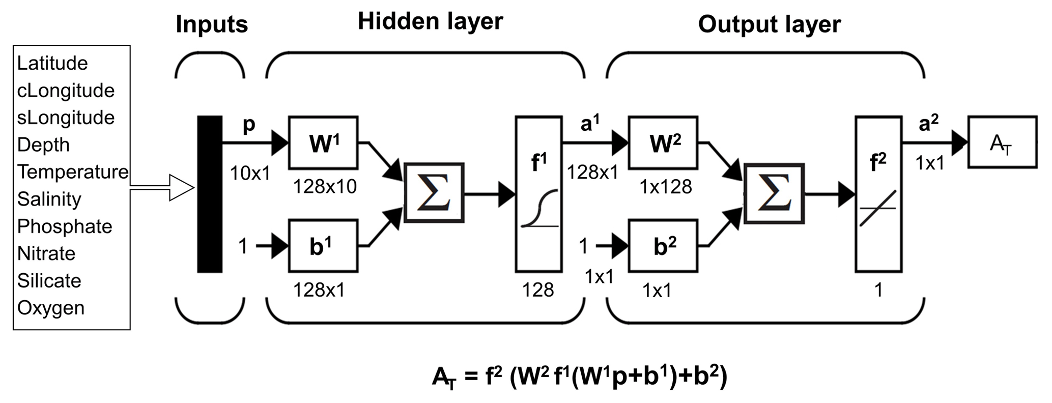
Figure 1Neural network configuration. The notation is in agreement with Hagan et al. (2014). p: input matrix; W: weight matrix; b: bias matrix; ∑: sum; f: transfer function; a: output matrix. The superscripts indicate the number of the layer. The cLongitude and sLongitude variables represent the cosine and the sine of longitude respectively (see Eqs. 2 and 3). The dimensions of the matrices are for an individual sample. Modified from Hagan et al. (2014).
The ability of the network to produce a reasonable output stems from a training process. Given a set of inputs and their targets, the network is trained to learn the relationships between both sets. The training process is possible due to a backpropagation training algorithm (Rumelhart et al., 1986). Generally, the network is initialized with random values of weights and biases, and an output is obtained. This output is compared with the target through a cost function, which typically is the mean squared error. Then the algorithm backpropagates this error through the network and iteratively adjusts the weights and biases to minimize the cost function. The minimization is commonly based on the Levenberg–Marquardt algorithm (Levenberg, 1944; Marquardt, 1963). Once the network is trained, output values can be obtained from a set of inputs with unknown targets. The more accurate and generalized the training data, the more accurate the output values.
The feed-forward neural network used in this study has a two-layer architecture. The first layer has a sigmoid transfer function and the second layer a linear transfer function (Fig. 1). This choice of functions allows both the linear and nonlinear relationships between AT and its predictors to be represented. This network configuration can approximate most functions arbitrarily well (Hagan et al., 2014). In the Atlantic Ocean, this arrangement has been shown to accurately estimate AT from diverse predictors (Velo et al., 2013).
The GLODAPv2 discrete data were used to train the network. Input variables (left hand in Fig. 1) were selected based on their potential influence on AT following Velo et al. (2013). They include the sampling position (coordinates and depth), temperature, salinity, nutrients (phosphate, nitrate and silicate) and dissolved oxygen. Position was included to help the network learn characteristic patterns associated with this input when the other variables cannot fully explain the AT variability. Takahashi et al. (2014) and Lee et al. (2006) showed how the relations between AT and the predictor variables used in these studies are different depending on the ocean area. The periodicity of the input longitude was represented by the equations used by Zeng et al. (2014):
Our approach only uses measured inputs from GLODAPv2, that is, those input data derived from the same rosette sample bottle as the AT value. Other studies with a similar approach take the inputs from reanalysis products or satellite data (e.g., Landschützer et al., 2013), which are inherently less accurate than direct measurements. The relations created by the network in the training procedure are likely to be more realistic using in situ-measured values for the input variables.
The samples where all input variables and AT were measured were selected from GLODAPv2 (https://www.nodc.noaa.gov/ocads/oceans/GLODAPv2_2019/, last access: 14 June 2019). From these, we removed the data where quality control (QC) was not done in all the variables (for a neural network trained with all data see Broullón et al., 2018). However, we keep all data from the Mediterranean Sea to adequately represent this sea in the climatology. The final dataset contained 251 687 samples. “GLODAPv2” hereinafter refers to the subset used in this study unless otherwise indicated.
Two different training techniques were tested: the Levenberg–Marquardt method (lm) and the Bayesian regularization (br) (both detailed in Hagan et al., 2014). In a similar study, Velo et al. (2013) demonstrated that these techniques give the best network performance among those which they tested. Except for the number of neurons, the two algorithms were implemented with the default options of the MATLAB functions trainlm and trainbr (detailed in Beale et al., 2018). These two functions prevent overfitting in different ways. The trainlm function usually needs to be fed with the data divided in three sets: a training set to obtain the relationships between variables, a validation set to prevent overfitting and a test set to compare different networks. Here, the training was stopped when the error in the validation set increased during six consecutive iterations of the training process to avoid overfitting. This process is known as early stopping (Hagan et al., 2014). The final values of the network weights and biases are those reached before the first of these iterations. The trainbr function adds a regularization parameter to the cost function to make the fit smoother in order to avoid overfitting. The validation set is not present in this technique. The end of the training is based on network convergence through parameter stabilization by an automatic process known as automated Bayesian regularization (Hagan et al., 2014; Beale et al., 2018). See Beale et al. (2018) and references therein for a detailed description of the two functions tested.
The number of network neurons is problem dependent with no fixed criterion for establishment. It is related to the complexity of the input–output mapping, the amount of training data available and their noise (Gardner and Dorling, 1998). Using too few neurons will not enable one to learn complex relations. Using too many neurons could overfit the data; that is, the network might model the uncertainty of the data used in the training. We determined the optimal number of neurons through a trade-off between the root-mean-squared error (RMSE) of the computed values and the generalization of the network. This last concept refers to network performance when a set of unused inputs is passed through the network to obtain an output. If the RMSE in this set is of the same order of magnitude as the RMSE in the training set, there is no substantial overfitting and the network generalizes well.
The training procedure was carried out in MATLAB. We tested 16, 32, 64, 128 and 256 neurons in the hidden layer based on the results of Velo et al. (2013). For each number of neurons, we trained 10 networks always using the same 90 % of GLODAPv2 for training (Fig. 2, first level). The remaining 10 % was used as an independent test set (Fig. 2, first level). Both subsets contained samples randomly distributed in the ocean to evaluate the maximum possible relationships between the input variables and AT through all oceanographic regimes, that is, to capture most of the variability in all the variables and not restricting the sets to specific areas. Each of the 10 networks starts the training procedure with random weight and bias values and a division of the training dataset into two portions: 85 % for training and 15 % for validation (Fig. 2, second level). The different starting points of the training process in the highly dimensional weight-error space make the minimization of the cost function different for each network. As each network is different, keeping all the sets allow one to determine which network best generalizes in the same test set. The selected network is the one that produces the lowest RMSE in the training data (Fig. 2, first level) and in the test data, considering a nonsignificant difference between both RMSEs to prevent overfitting. The network derived from this process will be referred to as NNGv2.

Figure 2Division of the data for the training of the network and its testing. The percentages in each level are relative to the previous one.
2.2 Comparison of methods
The relations proposed by Lee et al. (2006) and Takahashi et al. (2014) to generate a monthly surface climatology of AT from different predictors were applied over GLODAPv2. Lee et al. (2006) grouped AT data (<20–30 m depth) into five oceanographic regimes and obtained a best fit to a quadratic function of sea surface temperature (SST) and sea surface salinity (SSS) in each basin. Takahashi et al. (2014) divided the global ocean into 33 hydrographic provinces and expressed the potential alkalinity (PALK = AT + , <50 m depth) as a linear regression of salinity in 27 of them. PALK was used instead of AT for the purpose of eliminating seasonal biological effects, and the interprovince variation reflected differences in CaCO3 production in the mixed layer as well as the contributions of lateral and vertical mixing of waters. The analysis was carried out in the areas defined in the two studies.
The recent methods to compute AT proposed by Carter et al. (2018) and Bittig et al. (2018) (LIARv2 and CANYON-B respectively) were also compared to the one proposed here. LIARv2 is based on multilinear regressions (MLRs) including the same predictors used in the present study, excluding phosphate (sample position; salinity, S; potential temperature, θ; nitrate, N; apparent oxygen utilization, AOU; and silicate, Si). This method is composed of 16 equations with a different combination of the input variables, always maintaining the salinity input in each one. The computations with LIARv2 were obtained by the equation with the lowest uncertainty estimate in each sample that this method determines (Carter et al., 2018). CANYON-B is based on a Bayesian neural network derived from GLODAPv2 data including position, time, salinity, temperature and dissolved oxygen as predictors. The two methods were applied on the GLODAPv2 dataset and analyzed in the areas defined by Lee et al. (2006) and Takahashi et al. (2014).
2.3 Validation
To illuminate the complexity of neural networks, several methods to determine the contribution of each predictor variable in the output were proposed in different studies (see Gevrey et al., 2003 and Olden et al., 2004). We used the connection weight approach (Olden and Jackson, 2002) to evaluate if the network properly associates the AT variability with the predictor variables. This method was proposed to be the most accurate (Olden et al., 2004). It uses the weights obtained in the training stage to extract the influence of each predictor variable in fitting the AT values. The expression followed was
where Ci is the relative importance of the predictor variable i, H is the number of neurons in the hidden layer, wik is the weight of the connection between the variable i and the neuron k of the hidden layer, and wk is the weight of the connection between the neuron k of the hidden layer and the final output, that is, the computed AT. Finally, the absolute value of Ci was expressed as a percentage of the sum of all Ci.
In addition to the test in the GLODAPv2 independent set, the network potential was tested on five ocean time series in different oceanographic regimes that were not included in GLODAPv2: Hawaii Ocean Time-series (HOT), Bermuda Atlantic Time-series Study (BATS), European Station for Time-series in the Ocean at the Canary Islands (ESTOC), Kyodo North Pacific Ocean Time-series (KNOT) and K2. Data of all time series used in this study were obtained from https://www.nodc.noaa.gov/ocads/oceans/time_series_moorings.html (last access: 4 June 2019).
GLODAPv2 contains quality-controlled measurements in all ocean basins from the 1970s until 2017 (Olsen et al., 2019). However, winter data are scarce to absent in some high-latitude regions because adverse weather conditions prevents field activities in that season (Fig. S1 in the Supplement). In surface ocean, this temporal bias can be avoided with the help of the subsurface data from seasons with sufficient samples. Vázquez-Rodríguez et al. (2012) demonstrated how the subsurface ocean layer in the Atlantic Ocean can retain the footprint of the water mass formation from the preceding winter in the following months and, therefore, of the surface conditions. The winter relationships between inputs and AT needed to produce an all-season surface climatology are mostly preserved in this subsurface layer. The validity of this hypothesis was tested in other regions (Fig. S1) following Vázquez-Rodríguez et al. (2012). These areas were chosen based on the nonavailability of AT data in two or more consecutive months in the same oceanographic regime as the colored area in Fig. S1.
To reinforce the previous test and to assess the ability of the neural network in overcoming the lack of winter data in other depths, a neural network (NNGv2_nowinter) was trained excluding all winter data in GLODAPv2 (GLODAPv2_nowinter) and tested in the excluded and independent winter dataset (GLODAPv2_winter). The procedure to create and to train the network was the same as described previously.
2.4 Climatology
Finally, we generated a 1∘ × 1∘ global (monthly: 0–1500 m; annual: 1550–5500 m) climatology of AT from the objectively analyzed climatological fields of temperature, salinity and oxygen (see Appendix A for oxygen climatology) from WOA13 (Locarnini et al., 2013; Zweng et al., 2013; Garcia et al., 2014a) and the nutrients which resulted from passing the previous fields through CANYON-B (Appendix A). This choice of nutrients was made to extend the monthly resolution up to 1500 m, since WOA13 only offers it up to 500 m (Garcia et al., 2014b). This final product was compared with the monthly sea surface climatologies of AT of Lee et al. (2006) and Takahashi et al. (2014). Furthermore, the annual mean was compared with the annual mapped climatology by Lauvset et al. (2016) since it also comes from GLODAPv2. The availability in Lauvset et al. (2016) of the climatologies of the variables used as inputs in the network was used to test how the network represents the climatology of AT and to evaluate the sources of the possible differences.
3.1 Neural network analysis
The lowest RMSE was reached in the training and in the test sets when 128 neurons were used (Fig. S2). The same RMSE values for both sets (5.3 µmol kg−1; Figs. 3 and S2) showed that no overfitting occurred and that the network generalizes well. The two training techniques did not show significant differences. The Levenberg–Marquardt algorithm was selected for its higher computing speed.
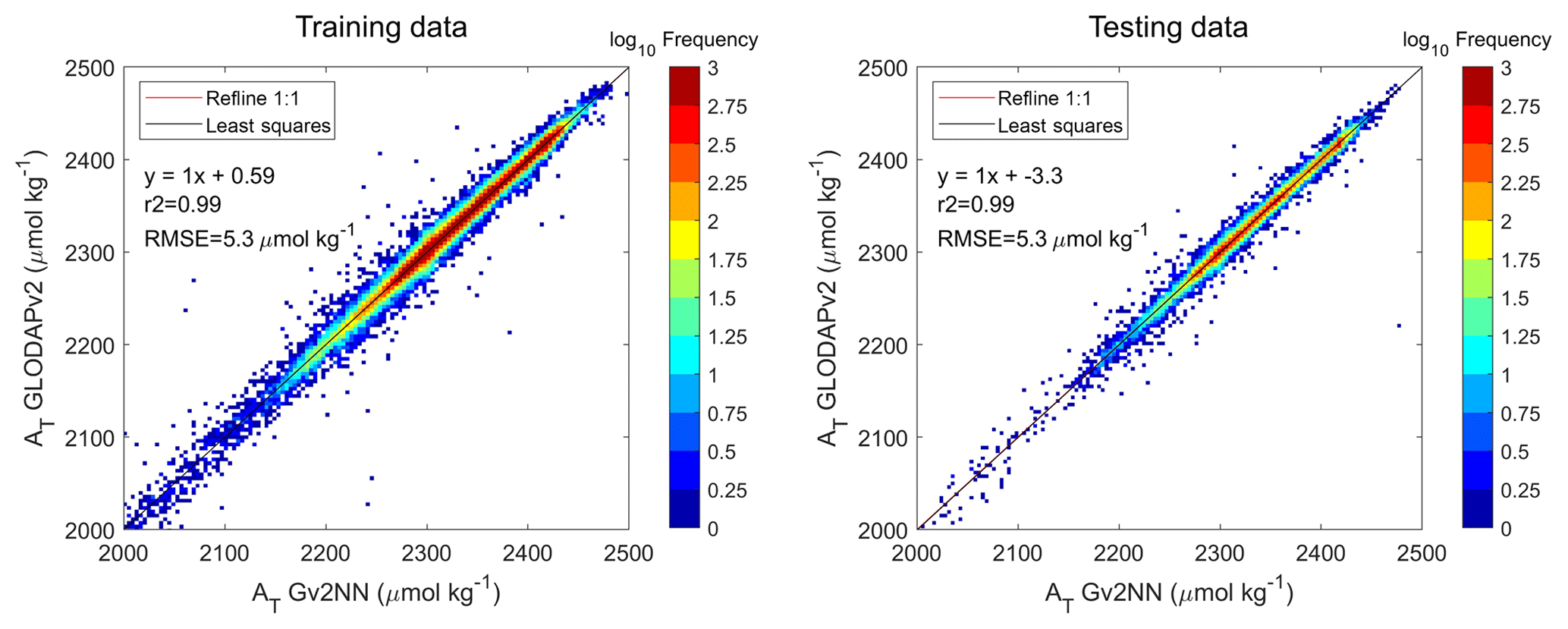
Figure 3Regression between AT computed by NNGv2 and AT from GLODAPv2. The graph is divided in pixels. The color of each pixel is determined by the number of points inside it. Each pixel has a size of 4 by 4 µmol kg−1. Note the logarithmic scale to account for the large amount of data. The training data chart contains the data in the first level training set (see Fig. 2). The testing data chart contains the data in the first level test set (see Fig. 2).
Samples with residuals (differences between measured and computed AT) beyond ± 3 RMSE (3 times RMSE; threshold selected to show samples with large residuals) are 1 % of the GLODAPv2 dataset. The spatial distribution of these samples (Fig. S3) shows that they are confined to certain areas, mainly in the ocean surface (Fig. 4). Most are in the Northern Hemisphere (Figs. S3 and 4). Specifically, 40 % are from latitudes north of 60∘ N (Table S1). In this area, 5 % of GLODAPv2 samples have residuals beyond ± 3 RMSE and 75 % of these samples are from the upper 100 m (Table S2). In these depth and latitude ranges, the samples with high residuals make up 13 % of the GLODAPv2 samples here and they typically have salinities lower than 34 (Table S3; Fig. S3). A monthly analysis in the previously indicated ranges shows that the largest number of samples with residuals beyond ± 3 RMSE are from the summer months. About 12 %–20 % of all GLODAPv2 samples from this season in this area have residuals higher than ± 3 RMSE (Table S4).

Figure 4The absolute differences between GLODAPv2 AT and NNGv2 AT. (a) Samples in the layer 0–30 m. (b) Samples in the layer 2950–3050 m.
The previous results show that the Arctic Ocean is the region with the largest RMSE, although the network computes most of the measured AT in this area well. However, the low availability of winter data, the ice–sea dynamics, and the transport of AT by the rivers (Fig. S4) could alter the presence of the surface winter conditions in the summer subsurface layer shown by Vázquez-Rodríguez et al. (2012) in other areas and generate a temporal bias in the climatology. The high discharge of high-AT waters by the rivers in the summer (Cooper et al., 2008; Shiklomanov et al., 2018; Fig. S5) generates the greatest errors and shows how the network fails to model riverine AT.
In further detail, many of the samples with residuals beyond ± 3 RMSE are located in the Beaufort Sea (66–80∘ N, 140–180∘ W). Here, Takahashi et al. (2014) also found a large RMSE of 60.5 µmol kg−1 (40.7 µmol kg−1 applying their regressions on GLODAPv2) for their SSS–PALK relations in the upper 50 m of the water column. This area is specifically complex to model surface AT because of significant river runoff having high and possibly variable AT concentrations (Figs. S4 and S5; Anderson et al., 2004; Cooper et al., 2008). The Labrador Sea also presents high errors because of the introduction of river runoff from Arctic Ocean transported through the Canadian Arctic Archipelago (Anderson et al., 2004). Therefore, in spite of the good reproduction of AT for the most samples, one should be cautious with the results in these zones and for the entire Arctic Ocean.
When the GLODAPv2 data where QC was not done are analyzed, the North Sea also shows many samples with large residuals. Those samples shallower than 100 m and close to the coasts surrounding this sea do not have an accurately computed AT (Fig. S4). Some studies have shown the complexity of the processes occurring in this shallow sea where the high river runoff also has elevated levels of AT (Fig. S4; e.g., Hoppema, 1990; Artioli et al., 2012). Hence, the same caveats as for the Arctic Ocean should be made.
In general, the network mainly fails to compute AT in some samples of areas with rivers carrying significant amounts of AT to the ocean. The inclusion of predictors related to riverine AT (and probably to ice melt) could improve the computation in these areas. Although one should be cautious, these zones still should be considered and be represented in the climatology since most of the samples have a well-computed AT.
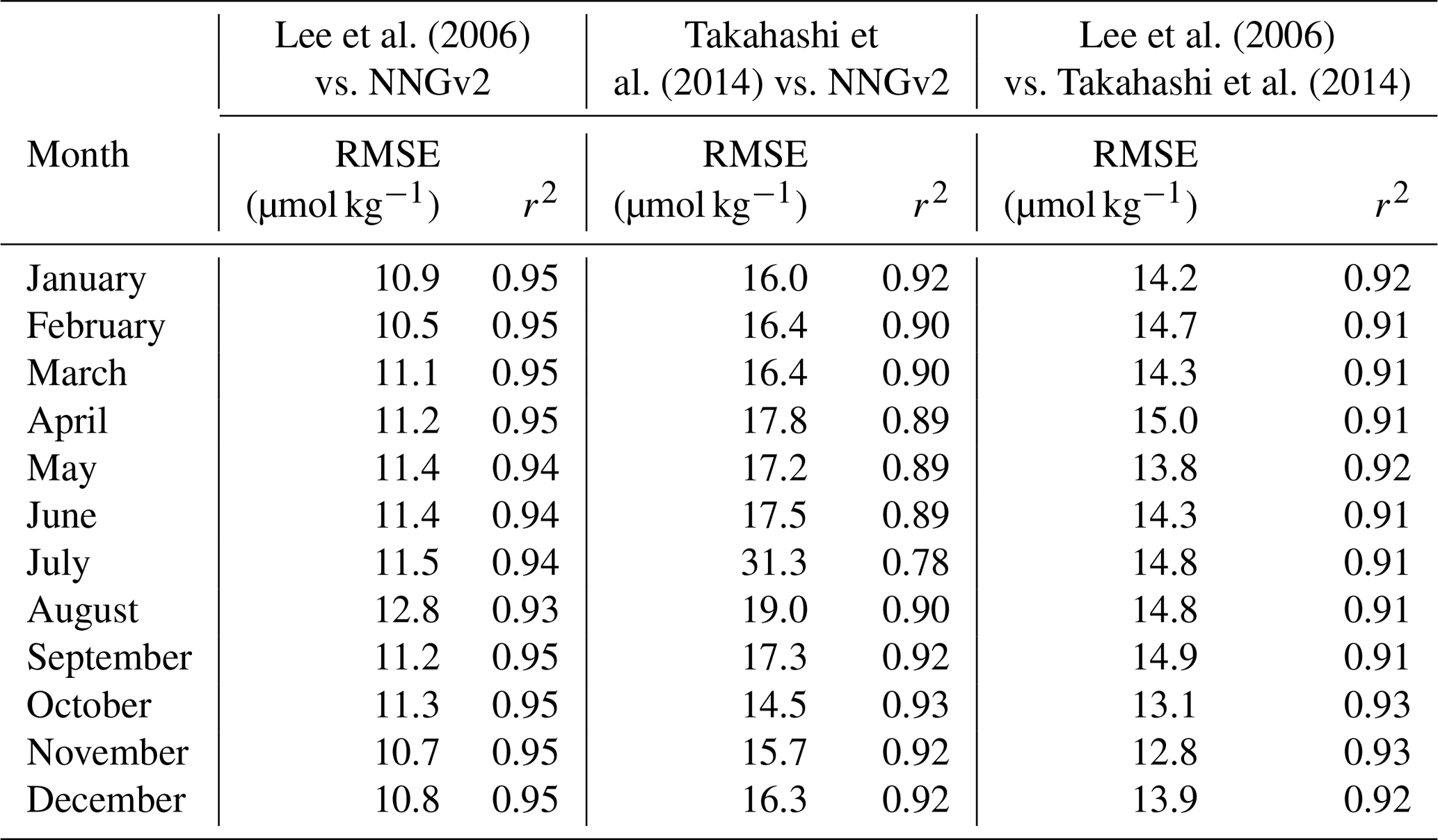
In the global ocean surface layer, the RMSE obtained with the neural network approach is lower than that obtained by previous studies on generation of monthly climatologies (Tables 1 and 2). In the past, relationships between SST and SSS with AT by Lee et al. (2006) have been shown to produce the lowest RMSE (area-weighted RMSE of 8.1 µmol kg−1) in the AT computation to create a monthly climatology. However, applying the relations of that study to GLODAPv2, the obtained weighted RMSE is higher than the ones from NNGv2, LIARv2 and CANYON-B (Table 1). The NNGv2 approach obtained the best fit in all the areas defined in the study of Lee et al. (2006) (Table 1). The newest methods in AT computation improve the results of Lee et al. (2006) in all the areas except for equatorial upwelling Pacific (CANYON-B) and subtropics (LIARv2) (Table 1).
Table 1RMSE obtained by the relations of Lee et al. (2006), NNGv2, LIARv2 and CANYON-B over GLODAPv2. The lowest RMSE in each area defined in Lee et al. (2006) is shown in bold. To be consistent with the surface layer defined in Lee et al. (2006) the samples evaluated here are from above 20 m (subtropics) and 30 m (the rest).
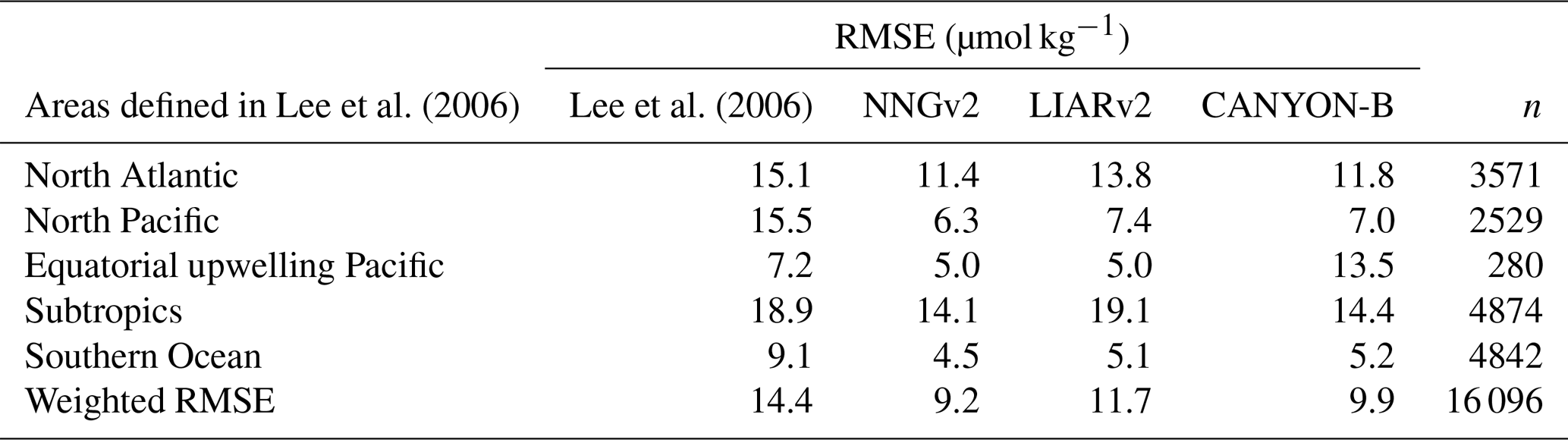
Table 2RMSE obtained by the relations of Takahashi et al. (2014), NNGv2, LIARv2 and CANYON-B over GLODAPv2. The lowest RMSE in each area defined in Takahashi et al. (2014) is shown in bold. To be consistent with the surface layer defined in Takahashi et al. (2014) the samples evaluated here are from above 50 m.
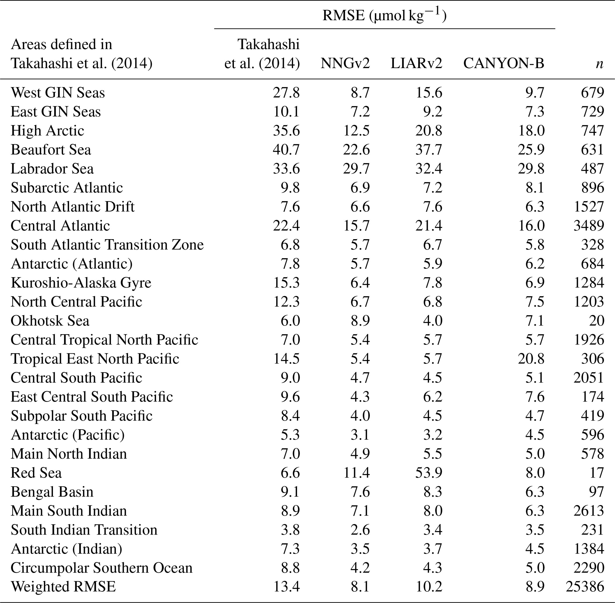
Similar to the previous case, the error analysis in the areas defined in Takahashi et al. (2014) also shows a lower error of the NNGv2 in most of the areas (20 of 26; Table 2). The weighted RMSE shows that NNGv2 and CANYON-B are the best methods to compute AT in the 0–50 m depth range in GLODAPv2. Although the analysis by area shows nonsignificant differences in general between these two methods, there are seven areas with more than 300 samples where NNGv2 computes AT with one or more units of RMSE less than CANYON-B. The AT computed in some zones defined in the Arctic and subarctic (Beaufort Sea and Labrador Sea) presents the highest RMSEs in all the approaches (Table 2), probably due to the high riverine AT discharge as discussed before.
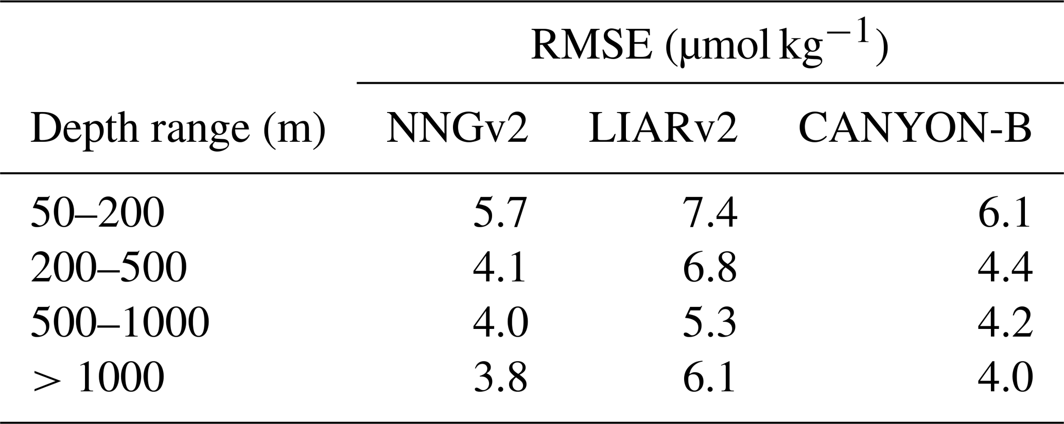
In depths below those previously analyzed, the error is progressively reduced for NNGv2, LIARv2 and CANYON-B (Table 3). Although NNGv2 shows the lowest RMSE in all the depth ranges analyzed, the differences with CANYON-B are nonsignificant. Nonetheless, LIARv2 shows higher errors than NNGv2 (between 1.3 and 2.6 µmol kg−1 higher; Table 3).
Table 3RMSE at different depth ranges obtained with NNGv2, LIARv2 and CANYON-B. Th lowest RMSE in each depth range is shown in bold.
The previous analyses show how the newest methods to compute AT (LIARv2, CANYON-B and NNGv2) produce lower errors than the previous ones used to generate a monthly climatology (Lee at al., 2006; Takahashi et al., 2014). The nonlinear nature of the neural networks is probably the main reason for the best results obtained with CANYON-B and NNGv2. Furthermore, these methods have the advantage of obtaining the computed AT anywhere in the ocean in only one step. No patches or smoothing are needed between different zones in the climatology as they are in previous studies. Finally, the NNGv2 has been chosen to generate the climatology because of both the previous reasons and the inclusion of data of recent cruises (Olsen et al., 2019) in the training and testing steps of the neural network approach.
The NNGv2 seems to qualitatively associate the AT variability with the predictor variables in coherence with the processes that contribute to it. The relative importance of these variables depicted in Fig. 5 shows that salinity is the most influential variable, followed by nutrients. In the surface layer, where AT variability is the largest, different studies showed how changes in salinity are highly correlated with this variability (Millero et al., 1998; Takahashi et al., 2014). The organic matter cycle also has a significant component in the AT variability (Kim and Lee, 2009). The formation and degradation of organic matter is reflected through both oxygen and nutrients variations. NNGv2 seems to capture the AT variability because of the organic matter cycle giving a second place in importance to nutrients. The third group of variables in the ranking of importance is comprised by position and temperature. The depth variable could be associated with the AT variability accounting for the variation produced by the CaCO3 cycle and the processes acting through the global ocean circulation. The horizontal sampling position variables could help to separate the different relations shown by previous studies in different ocean areas (Lee et al., 2006; Takahashi et al., 2014). Finally, temperature has also been associated with the AT variability as a proxy of both the CaCO3 and the organic matter cycles (Lee et al., 2006).
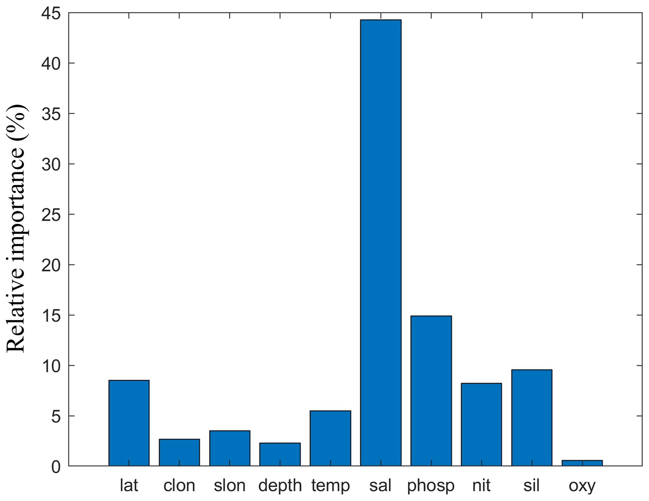
Figure 5The relative importance of the predictor variables for NNGv2. lat: latitude; clon: Eq. (3); slon: Eq. (4); temp: temperature; sal: salinity; phosp: phosphate; nit: nitrate; sil: silicate; oxy: oxygen.
3.2 Time-series validation
The network can compute AT well at five different ocean time-series stations. Low RMSEs (Table 4) and high coefficients of determination (r2) (data not shown) were obtained. The bias is relatively low in the three time series with the highest number of data (HOT, BATS and ESTOC). The AT computed by the NNGv2 in KNOT and K2 is slightly higher than the measured one, probably because of the influence in the AT variability of some variable not included as an input of the network (although an offset in the measurements of any of the inputs could also give this result). Summed to the previous test, the statistics obtained in this independent test with a good seasonal time resolution show the good generalization of the NNGv2.
Table 4RMSE and bias between measured AT in HOT, BATS, ESTOC, KNOT and K2, as well as the computed AT with NNGv2, LIARv2 and CANYON-B. The comparison was done for all the samples where all the input variables for NNGv2 and the AT were measured in the same water sample.
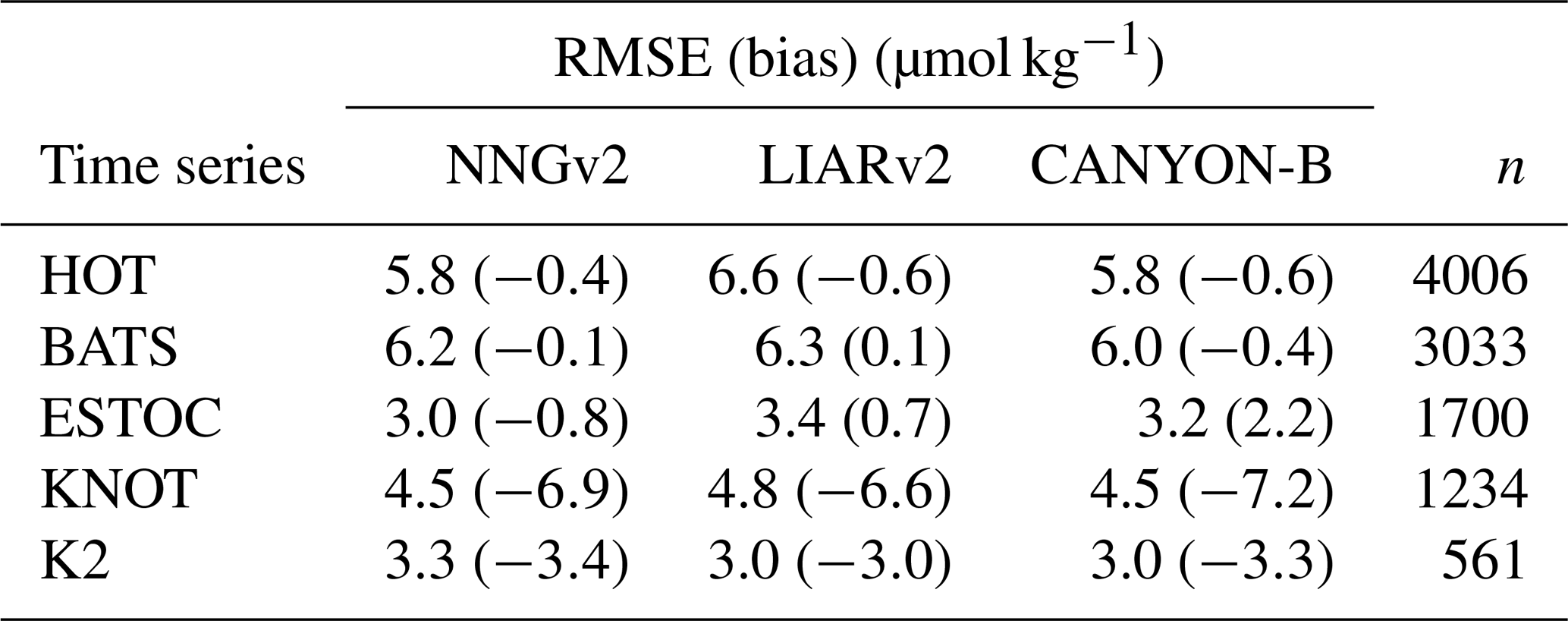
The LIARv2 and CANYON-B methods to compute AT also model the time-series data quite well (Table 4). Significant differences among the three methods are obtained in HOT and ESTOC. In HOT, NNGv2 and CANYON-B reach a better fit of AT than LIARv2, suggesting that a nonlinear technique is more adequate to model AT in this area (Table 4). CANYON-B presents a higher bias in ESTOC than the other two methods, suggesting that here the inclusion of nutrients as predictors results in an accurate computation of AT. The error obtained in BATS, ESTOC, K2 and KNOT does not have significant differences between methods. Finally, LIARv2 and CANYON-B also have a considerable bias in K2 and KNOT (Table 4) that reinforces the two reasons suggested previously for NNGv2.
The ability of NNGv2 to capture surface AT variability is exemplified in Fig. 6 for BATS. The other largest time series also show a good agreement between the computed and the measured seasonal AT in the same depth range (RMSE HOT: 5 µmol kg−1; RMSE ESTOC: 2.6 µmol kg−1). In general, AT's measured in each month of the year are well modeled by NNGv2 (inner charts in Fig. 6). The same holds for other depth layers (Fig. 7b, c, e and f). Only some extreme values are not fully captured, but almost all the trends between months are well represented. The differences may be caused by bias in measured AT or some of the input variables; they may also be due to an under-/overestimation of the network. Furthermore, the time-series areas are not fully represented in all months in GLODAPv2, so NNGv2 might not represent seasonality well. However, the network computes AT in any month with a very low error. This shows again the potential of the generalization of a well-designed neural network.
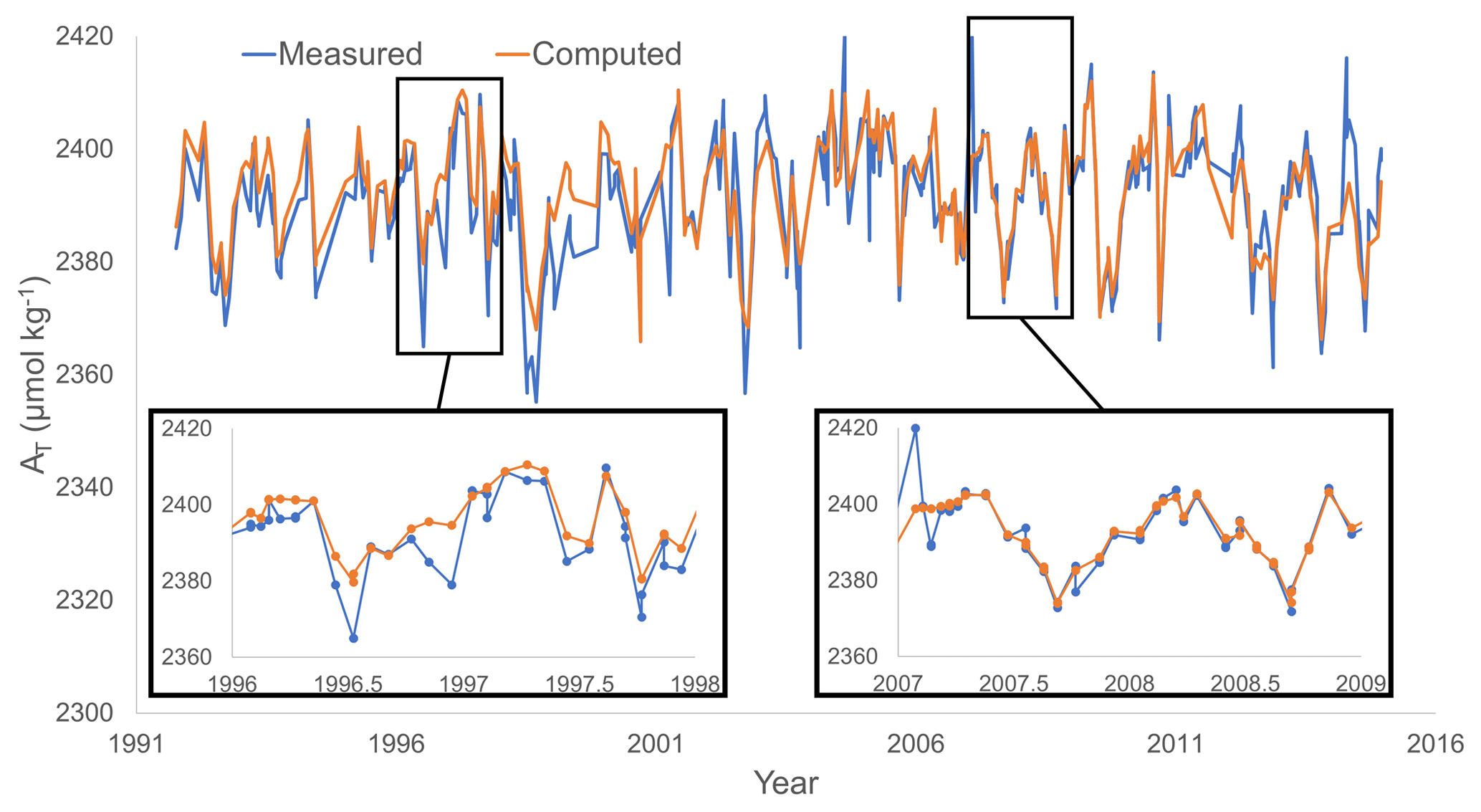
Figure 6Comparison of measured and computed AT with NNGv2 for the depth range 0–10 m at time-series station BATS. The RMSE in that depth range for the whole time period is 5.6 µmol kg−1. The years 1996–1997 and 2007–2008 are amplified to show the monthly variations because they are the years with AT measurements in all the months.
The NNGv2 also has the capacity to increase the number of AT data in the time series. In many samples, AT was not measured but the other input variables needed for the NNGv2 are available. Therefore, the computed AT has a higher temporal and spatial resolution than observations only. This enables the computation of more reliable trends than with the less frequently measured AT and allows the identification of possible high-frequency changes. The improvement in resolution is especially visible in the longer time series: HOT and BATS (Fig. 7). In the former we increased the number of AT data from 4006 to 14907 and in the latter from 3033 to 11 342 (Fig. 7b and e).
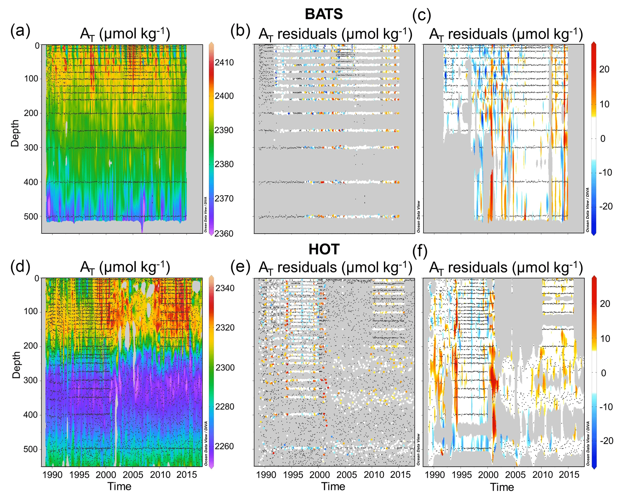
Figure 7(a, d) Computed AT for the upper 550 m of the water column at the BATS and HOT time-series stations. (b, e) Difference between measured and computed AT. Colored dots show samples where AT was measured. Black dots show samples where AT was not measured but the network inputs were. (c, f) Difference between measured and computed AT interpolated with Data-Interpolating Variational Analysis (DIVA; Troupin et al., 2010). This figure was made with Ocean Data View (Schlitzer, 2016).
3.3 Subsurface layer hypothesis
We found that the optimal depth range of the subsurface layer defined by Vázquez-Rodríguez et al. (2012) for the North Atlantic Ocean (100–200 m) must be modified in other regions. In the area analyzed in the Indian Ocean (Fig. S1), the subsurface layer hypothesis is verified in the same depth range of that study. However, the other areas (Fig. S1) show that the range of the subsurface layer is 50–100 m. The different strengths of deep mixing and convection in winter could explain this fact.
The properties analyzed in the four areas defined in Fig. S1 show, as expected, a higher monthly variability in the ocean surface than in the subsurface layers. The seasonal variability depicted in Fig. 8 will likely be typical of a larger region within a similar oceanographic regime for each defined area. The surface winter conditions of the analyzed properties are quite similar to those in the subsurface layer during, at least, one of the four consecutive months following winter in all areas (Fig. 8).

Figure 8Monthly variability of temperature, salinity, NO = 9*NO3 + O2 and PO = 135*PO4 + O2 (defined according to Broecker, 1974) for different ocean basins. All variables were averaged for each area defined in Fig. S1. Temperature and salinity were obtained from WOA13 objectively analyzed monthly climatologies, oxygen was obtained filtering the WOA13 objectively analyzed monthly climatology (see Appendix A), nitrate and phosphate were obtained by applying CANYON-B to the previous variables (see Appendix A), and AT was obtained from the present climatology (see Sect. 3.4). Each zone is displaced in each graph for a certain constant quantity of the variable for a better visualization; that is, the data shown are not the real values. Indian Ocean: 100–200 m; South Atlantic, South Pacific and North Pacific: 50–100 m.
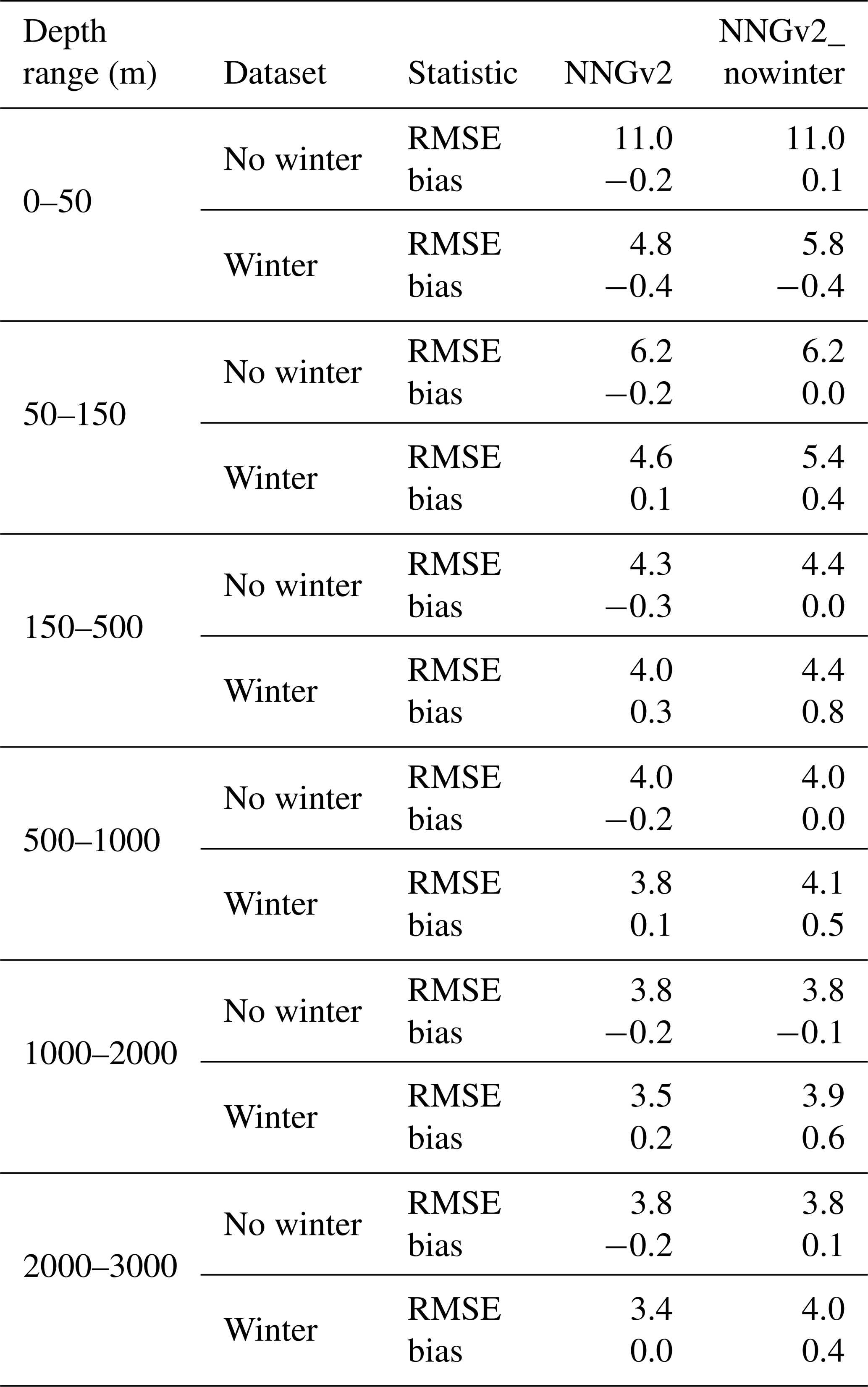
The optimal number of neurons in the network trained with the GLODAPv2_nowinter dataset to reinforce the subsurface layer hypothesis and to assess the layers below surface ocean was 100. The reduction of the number of neurons compared to the previous networks was because this new dataset contains less data. Thus, maintaining or increasing the number of neurons used for NNGv2 would produce overfitting. NNGv2_nowinter provides statistics in the GLODAPv2_nowinter dataset similar to those of the NNGv2 in GLODAPv2 dataset (5.5 vs. 5.3 µmol kg−1 respectively). But of greater importance are the statistics which resulted from the GLODAPv2_winter dataset, which reinforce the subsurface layer hypothesis (Table 5). The low error reached in this independent winter dataset and the low differences with that from NNGv2 in each depth layer (Table 5) show how the network is able to obtain the winter relations in any depth from the function fitted with data from other seasons. Therefore, the lack of winter data in different regions does not automatically mean that the climatology will be biased towards the more sampled seasons.
Table 5RMSE and bias obtained with NNGv2 and NNGv2 in different depth ranges and datasets of GLODAPv2. Units are micromoles per kilogram (µmol kg−1).
3.4 Climatology
The monthly climatology of AT is based on the relations obtained in the training procedure of NNGv2 applied to the WOA13 and CANYON-B-derived monthly climatological fields (Appendix A). We have demonstrated that the AT computed by NNGv2 agrees reasonably with the measured AT when the inputs associated with it are passed through the network; i.e., the relations obtained from GLODAPv2 in the training stage are robust. Therefore, the AT patterns in the climatology are forced by the patterns of the WOA13 variables and CANYON-B-derived ones used as inputs. The climatology can be found in a netCDF file at the data repository of the Spanish National Research Council (CSIC; https://doi.org/10.20350/digitalCSIC/8644; Broullón et al., 2019) together with a video of the monthly variation at the surface and in three longitudinal sections of the three main oceans.
The distribution of the surface annual mean AT (Fig. 9) is similar to that shown in previous climatologies (e.g., Lee et al., 2006; Takahashi et al., 2014; Lauvset et al., 2016). Not surprisingly, there is a high correlation with the salinity distribution and, consequently, with the evaporation–precipitation patterns. The largest values in the surface layer occur in the Mediterranean Sea, Red Sea, and in the subtropical gyres of the Atlantic and South Pacific Ocean, with all of them prevailing throughout the year in the monthly climatology. At depth, these maxima are all present at least up to 150 m (Fig. 9). Below 700 m, the Pacific and Indian Ocean show higher AT concentrations than the younger waters of the Atlantic (Fig. 9). Furthermore, features such as the high-AT Mediterranean water entering the Atlantic Ocean are captured in the climatology (Fig. 9, 1000 m chart, black circle). In general, the patterns agree with the main ocean processes responsible for the AT variability as explained previously.

Figure 9Annual mean climatology of AT at three depths. The black circle in the 1000 m panel points out the area of influence of the Mediterranean water in the Atlantic Ocean. This figure was made with Ocean Data View (Schlitzer, 2016).
The seasonal amplitude of sea surface AT (Fig. 10) is generally in agreement with that obtained by Lee et al. (2006). The highest amplitudes are in the north equatorial zone, in the Arctic Ocean and in coastal zones, i.e., at locations where there are rivers with a large water discharge (like the Amazon, Congo, La Plata or Arctic rivers). The seasonal amplitude of the surface salinity (Fig. S6) can explain most of the variability in the seasonal amplitude of AT. In areas with a large seasonal amplitude of salinity (more than 1 unit; mainly the Arctic Ocean and coastal zones near rivers with high discharge), this variable linearly explains 79 % of the seasonal amplitude AT variability. However, the seasonal amplitude in the Arctic Ocean should be taken with caution due to the difficulty in accurately modeling this complex zone, as discussed previously. Despite the presence of high levels of AT in some river mouths in the melting months, the AT carried by the rivers could not be represented in the climatology, and this can enhance the seasonal cycle due to an underestimated value in low-salinity waters with high riverine AT. On the other hand, in areas with a low seasonal amplitude of salinity (less than 1 unit; mainly oceanic areas and coastal regions without rivers with high discharge), about 62 % of variability is linearly explained. This result shows the importance of the inclusion of other predictors besides salinity in the network and the nonlinearity of the method proposed in this study to explain nearly all the AT variability.
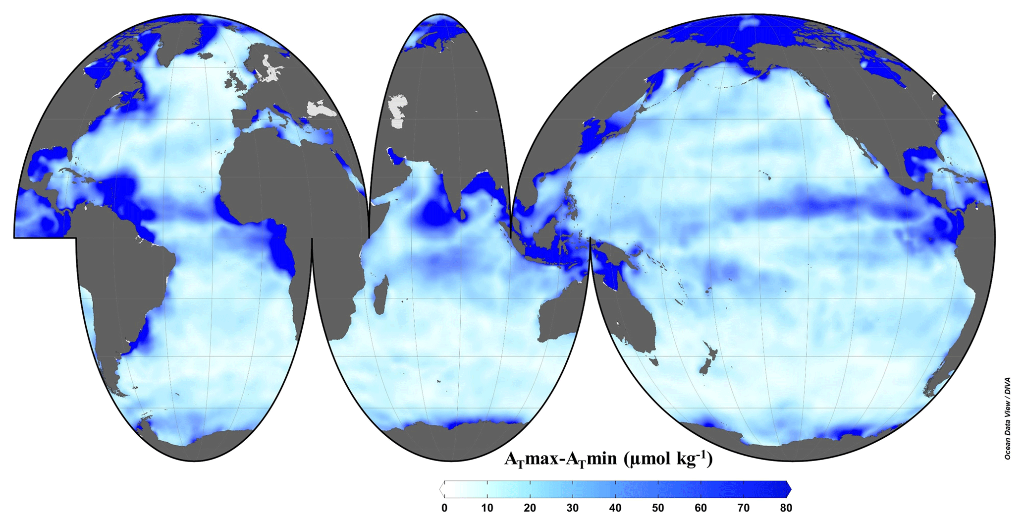
Figure 10Seasonal amplitude of sea surface AT. This figure was made with Ocean Data View (Schlitzer, 2016).
The seasonal amplitude of AT is progressively reduced at depth (Fig. S7) as a result of the reduction of the variability of the variables which influence the variability of the AT. The seasonality disappears almost completely below 400 m depth, although some patches of variability are present likely because of a conjunction of the error of the network and the seasonal variability in the climatological input variables. In addition, these patches could also come from the learning stage since the training data of AT present monthly variations of up to ∼15 µmol kg−1 for some areas, even at depths greater than 1000 m.
Although it was shown that the neural network can accurately compute AT in both GLODAPv2 and time-series datasets, the quality of WOA13 data (and that of the input climatologies generated in this study) also determines the robustness of the climatology. Unfortunately, WOA13 does not offer uncertainty fields associated with the objectively analyzed climatologies to compute a coherent estimation of the uncertainty in the AT climatology. Therefore, the climatological values offered in this study should be evaluated by comparing them with observations in a monthly average over many years. This can only be done at the locations of time series with representative amounts of data; Fig. 11 shows this analysis at the surface. At both the BATS and HOT time series, the differences between the averaged measured AT and the climatology are quite low. The comparisons are better when AT is computed by NNGv2 using as inputs the measured values in the time series (data not shown), showing the importance of the quality of the input variables.
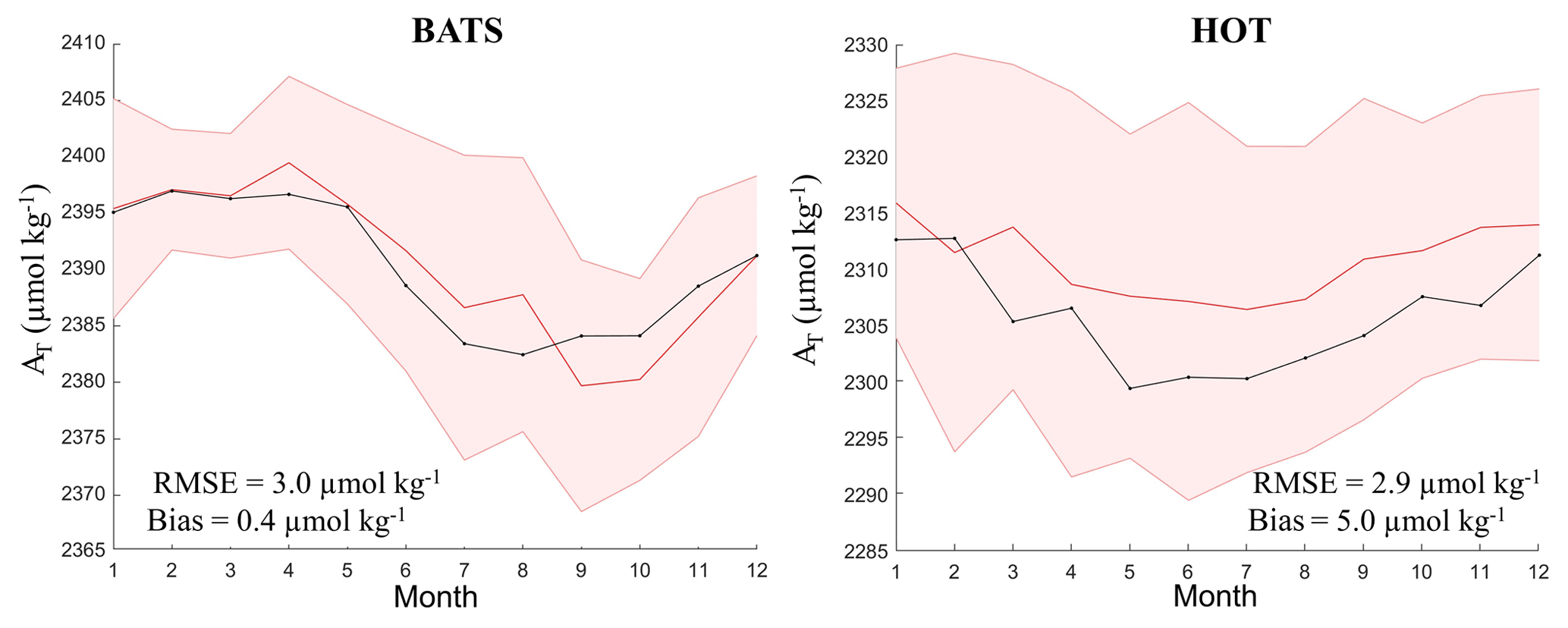
Figure 11Monthly variation of AT at BATS (0–10 m) and HOT (0–30 m) time-series locations of climatological measured data (red line) and the monthly climatology of AT computed with NNGv2 (black line). The shading represents the standard deviation of the average of the measured data.
The previous results hold true also for other depth layers. A comparison of monthly profiles up to about 500 m (BATS) and 1000 m (HOT) between the AT climatology obtained from WOA13 and CANYON-B-derived climatological fields and the one from the averaging of the time-series data shows low differences (Fig. S8). In BATS, the RMSE of this comparison ranges between 1.4 and 3.6 µmol kg−1 (mean RMSE of 2.2 µmol kg−1) and the bias between −0.2 and 4.3 µmol kg−1 for all months. In HOT, the RMSE of this comparison ranges between 3.6 and 9.7 µmol kg−1 (mean RMSE of 6.3 µmol kg−1) and the bias between −1.7 and 3.1 µmol kg−1 for all months. The climatological measured data are for the periods between 1991 and 2015 (BATS) and between 1989 and 2018 (HOT), and WOA13 data are supposed to cover a larger range. Despite this time difference, the AT climatology represents quite accurately the measured values averaged in each month.
Compared to the other climatologies, the surface annual mean AT of this study is closer to that of Lee et al. (2006) (Table 6). This is likely because temperature and salinity are included as nonlinear predictors of AT. In Takahashi et al. (2014), AT derives from the linear regression between PALK and one predictor (salinity), and in the Lauvset et al. (2016) study DIVA (Data-Interpolating Variational Analysis; Troupin et al., 2010) was used. Furthermore, the transfer of our climatology to the coarser grid of Takahashi et al. (2014) for the comparisons may enhance dissimilarities.
Table 6Comparison of four annual mean surface climatologies of AT. * The domain analyzed is the same as Lee et al. (2006) for coherency reasons.

The comparison of the monthly values of our climatology and the other climatologies available at the same time frequency (Table 7) shows the greatest similarity of ours and that of Lee et al. (2006). The reasons given above may also hold here. In addition, part of the differences between the comparisons may originate from the different versions of the WOA used in each study (Lee et al., 2006: temperature and salinity from WOA01; Takahashi et al., 2014: salinity from WOA09 and nitrate from WOA94; this study: temperature, salinity and oxygen (filtered) from WOA13 and nutrients derived from CANYON-B (Appendix A)).
Table 7Comparison between the three monthly climatologies of AT.
In general, the surface spatial patterns of the differences between the annual mean of our AT climatology and the three other ones under consideration are not correlated (Fig. S9). Compared to Takahashi et al. (2014), the largest differences are in the Beaufort Sea and in three zonal bands: 54–60∘ S, 8–28∘ N and 40–60∘ N (Fig. S9a). The Pacific Ocean has the highest dissimilarities in these three bands. In general, the Atlantic Ocean and the Indian Ocean have the smallest differences. The largest differences in these two ocean basins are mainly located close to the river mouths. This result shows how the different parametrizations of the AT diverge highly at low salinities. On the other hand, the major differences with Lee et al. (2006) (Fig. S9b) are surrounding North America's Pacific coast, the area of influence of the Amazon river, the zone between both the Niger and the Congo rivers, and the North Sea. In the open ocean there are some wide areas where the differences are remarkably high. They are mainly in the South Pacific. It should also be noted that the transition zone between areas 1 (subtropics) and 2 (equatorial upwelling Pacific) defined in the study of Lee et al. (2006) generates a discontinuity in the difference map. Finally, the largest differences with Lauvset et al. (2016) (Fig. S9c) are less localized. The Arctic Ocean and the Pacific sector of the Southern Ocean are the areas where there is a large spatial continuity in the differences.
An important cause of the differences between the climatologies stems from the use of different inputs to generate them. As an example, this can be seen when the climatologies of Lauvset et al. (2016) are used as input variables to compute AT with NNGv2 instead of the WOA13 data. In the surface layer, a considerable reduction of the RMSE (12.9 to 9.9 µmol kg−1) and an increase of the r2 from 0.94 to 0.96 are obtained. In the deeper layers, the differences are progressively decreasing. The values of the RMSE of the comparisons below 250 m are in the range of 4 to 6 µmol kg−1, and the improvement caused by the input usage is reduced to around 1 µmol kg−1. This last result shows an increasing similarity between Lauvset et al. (2016) climatologies and those used in the present study with increasing depth. However, and to be consistent, it is recommended to use the AT climatology corresponding with the other inputs used in the studies that arise from these products (e.g., biogeochemical modeling studies).
The climatologies of AT, oxygen and nutrients (see Appendix A) and the NNGv2 designed in this study are available at the data repository of the Spanish National Research Council (CSIC; https://doi.org/10.20350/digitalCSIC/8644, Broullón et al., 2019).
A neural network to compute AT anywhere in the ocean has been presented. As evaluated by the RMSE between the measured and the computed data, the neural network approach presented in this study offers increased precision compared to most of the approaches in previous studies. Furthermore, the global relationship between AT and input variables was obtained from a higher number of quality-controlled data than before in the generation of a monthly climatology, with a greater temporal and spatial resolution. We have demonstrated how one single global algorithm is able to compute AT satisfactorily for the entire global ocean. This has enabled us to generate a monthly climatology without the need to use smoothing techniques between different oceanic areas.
The validation using different independent datasets demonstrates the good network generalization. In addition, the spatiotemporal AT variability is well captured by the network as shown in time-series validation. Therefore, the obtained climatology using WOA13 inputs and those of oxygen and nutrient climatologies created in this study should reflect this variability due to the good network performance in the independent datasets.
We offer this global monthly climatology of AT to the scientific community for advancing the understanding of the ocean carbon cycle. Our new climatology may be particularly useful as input to modeling efforts. It is worthwhile to mention that the network offered here is also useful to obtain AT values for samples where the inputs for the neural network are present.
The relevance of a well-represented seasonal variability in the predictor variables used to create the monthly AT climatology is very important to obtain a well-represented AT seasonal variability. Analyzing the variability in the WOA13 variables, we have found some remarkable aspects that have led us to modify and generate new climatologies for some of the predictor variables.
When the variability in WOA13 climatologies is compared with the one in time series with enough measured data to obtain climatological values, a strange variability is observed in the former. In general, the monthly climatologies of oxygen and nutrients present some high peaks of seasonal variability at different depths in relation to the neighboring depths around all of the ocean. These peaks also occur at time series locations showing a discrepancy regarding the measured climatological seasonal variability (Figs. A1 and A2).
The profile of oxygen seasonal variability at ESTOC clearly shows this fact at depths around 750 and 1200 m (Fig. A1). The same happens at ICELAND around 800 m, although with a smaller magnitude (Fig. A1). To avoid the disruptions in the profiles of oxygen seasonal variability, we applied a fifth-order one-dimensional median filter through the depth dimension to the WOA13 oxygen monthly climatology. In general, the results show a reduction of the peaks, and the trends and magnitude of the profiles are more similar to those of the measured data (Fig. A1).
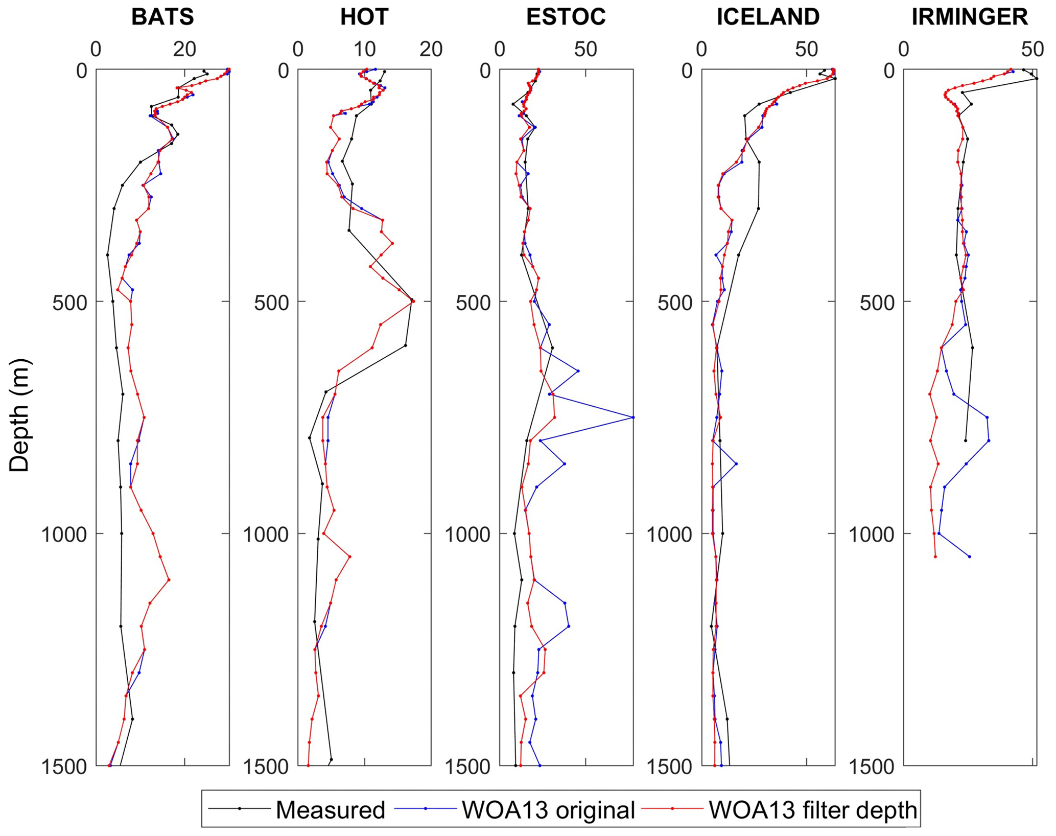
Figure A1Profiles of oxygen seasonal amplitude at different time-series locations obtained from WOA13 oxygen monthly climatology (WOA13 original), from WOA13 original after a median filtering (WOA13 filter depth) and from measured data averaged by month (Measured). It should be considered that profiles at ESTOC, ICELAND and IRMINGER do not come from a quantity of data as high as those of HOT and BATS and cannot be considered a pure climatology. Units of seasonal amplitude are micromoles per kilogram (µmol kg−1).
In the case of nutrients, we took advantage of the recent publication of the CANYON-B method (Bittig et al., 2018) which allows one to compute phosphate, nitrate and silicate from temperature, salinity, oxygen, position and time. Therefore, the monthly climatologies of temperature and salinity from WOA13 and the one of oxygen created in this study were used as inputs of CANYON-B to obtain monthly climatologies of nutrients up to 1500 m (this depth is the maximum depth up to which WOA13 offers monthly climatologies of temperature, salinity and oxygen). In general, the results show a reduction of the peaks shown by WOA13 and a higher similarity with the measured profiles (Fig. A2).
The monthly climatologies of oxygen and nutrients from WOA13 probably present the mentioned disruptions of the seasonal variability because of a combination of low data availability in certain areas and the method used for mapping. Therefore, the monthly climatology of AT obtained using as inputs of the NNGv2 the climatologies created here should represent a more realistic seasonal variability than if all WOA13 ones were used.
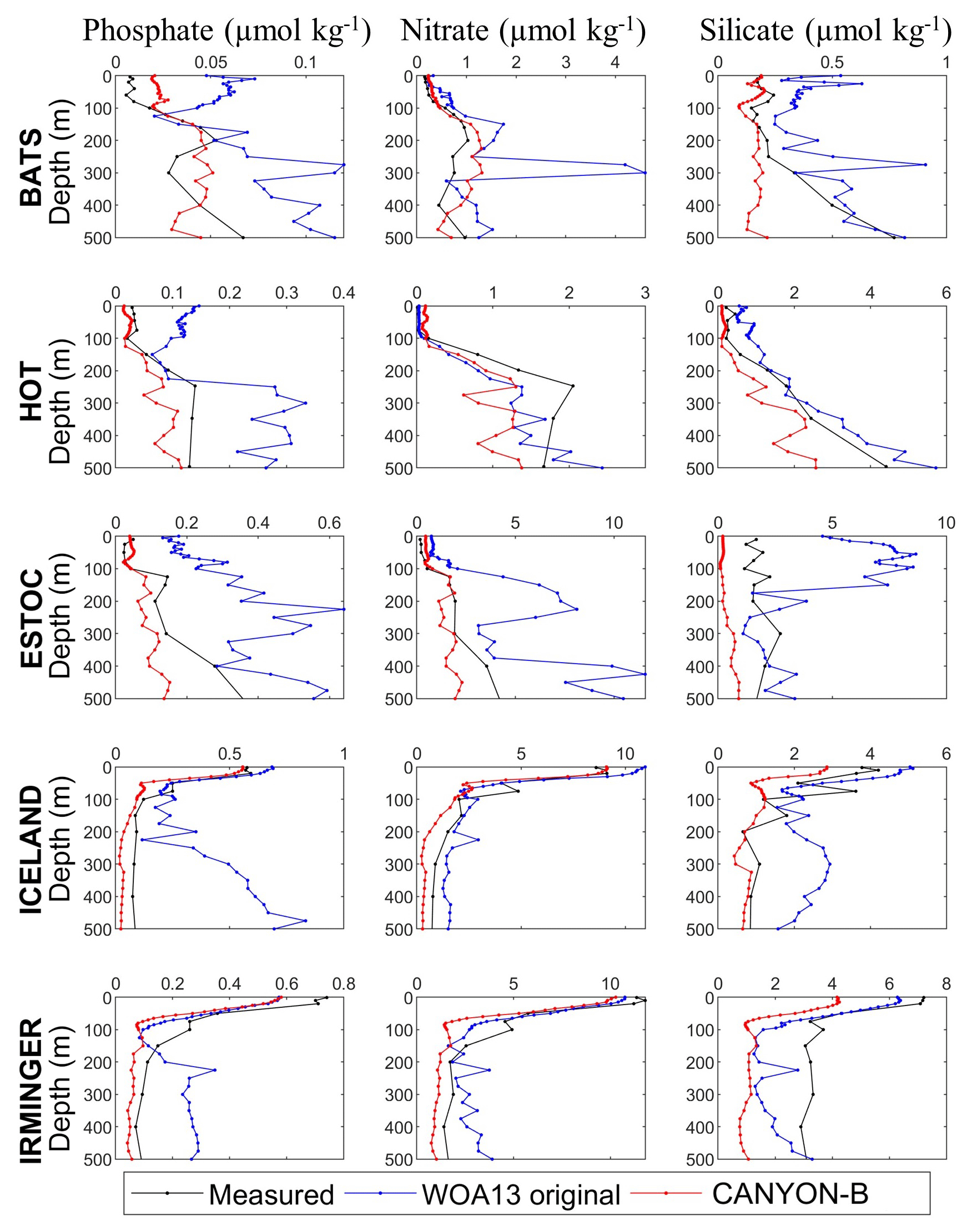
Figure A2Profiles of nutrient seasonal amplitude at different time-series locations obtained from WOA13 monthly climatologies (WOA13 original), CANYON-B-derived climatologies (CANYON-B) and from measured data averaged by month (Measured). It should be considered that profiles at ESTOC, ICELAND and IRMINGER do not come from a quantity of data as high as those of HOT and BATS and cannot be considered a pure climatology.
The supplement related to this article is available online at: https://doi.org/10.5194/essd-11-1109-2019-supplement.
DB, FFP and AV designed the study. The manuscript was written by DB and revised and discussed by all the authors. The dataset of the climatology and the neural network were created by DB.
The authors declare that they have no conflict of interest.
The authors want to thank the comments of Siv K. Lauvset and of the three anonymous referees to improve the manuscript.
This research has been supported by the H2020 Food (AtlantOS, grant no. 633211); the Ministerio de Educación, Cultura y Deporte (grant no. FPU15/06026); the Ministerio de Economía y Competitividad, Consejo Superior de Investigaciones Científicas (grant no. CTM2016-76146-C3-1-R); and the Ministerio de Economía y Competitividad, Salvador de Madariaga (grant no. PRX18/00312).
This paper was edited by David Carlson and reviewed by three anonymous referees.
Anderson, L. G., Jutterström, S., Kaltin, S., Jones, E. P., and Björk, G.: Variability in river runoff distribution in the Eurasian Basin of the Arctic Ocean, J. Geophys. Res., 109, 1–8, https://doi.org/10.1029/2003JC001773, 2004.
Artioli, Y., Blackford, J. C., Butenschön, M., Holt, J. T., Wakelin, S. L., Thomas, H., Borges, A. V., and Allen, I.: The carbonate system in the North Sea: sensitivity and model validation, J. Mar. Syst., 102–104, 1–13, https://doi.org/10.1016/j.jmarsys.2012.04.006, 2012.
Bakker, D. C. E., Pfeil, B., Landa, C. S., Metzl, N., O'Brien, K. M., Olsen, A., Smith, K., Cosca, C., Harasawa, S., Jones, S. D., Nakaoka, S.-I., Nojiri, Y., Schuster, U., Steinhoff, T., Sweeney, C., Takahashi, T., Tilbrook, B., Wada, C., Wanninkhof, R., Alin, S. R., Balestrini, C. F., Barbero, L., Bates, N. R., Bianchi, A. A., Bonou, F., Boutin, J., Bozec, Y., Burger, E. F., Cai, W.-J., Castle, R. D., Chen, L., Chierici, M., Currie, K., Evans, W., Featherstone, C., Feely, R. A., Fransson, A., Goyet, C., Greenwood, N., Gregor, L., Hankin, S., Hardman-Mountford, N. J., Harlay, J., Hauck, J., Hoppema, M., Humphreys, M. P., Hunt, C. W., Huss, B., Ibánhez, J. S. P., Johannessen, T., Keeling, R., Kitidis, V., Körtzinger, A., Kozyr, A., Krasakopoulou, E., Kuwata, A., Landschützer, P., Lauvset, S. K., Lefèvre, N., Lo Monaco, C., Manke, A., Mathis, J. T., Merlivat, L., Millero, F. J., Monteiro, P. M. S., Munro, D. R., Murata, A., Newberger, T., Omar, A. M., Ono, T., Paterson, K., Pearce, D., Pierrot, D., Robbins, L. L., Saito, S., Salisbury, J., Schlitzer, R., Schneider, B., Schweitzer, R., Sieger, R., Skjelvan, I., Sullivan, K. F., Sutherland, S. C., Sutton, A. J., Tadokoro, K., Telszewski, M., Tuma, M., van Heuven, S. M. A. C., Vandemark, D., Ward, B., Watson, A. J., and Xu, S.: A multi-decade record of high-quality fCO2 data in version 3 of the Surface Ocean CO2 Atlas (SOCAT), Earth Syst. Sci. Data, 8, 383–413, https://doi.org/10.5194/essd-8-383-2016, 2016.
Bates, N., Astor, Y., Church, M., Currie, K., Dore, J., Gonaález-Dávila, M., Lorenzoni, L., Muller-Karger, F., Olafsson, J., and Santa-Casiano, M.: A Time-Series View of Changing Ocean Chemistry Due to Ocean Uptake of Anthropogenic CO2 and Ocean Acidification, Oceanography, 27, 126–141, https://doi.org/10.5670/oceanog.2014.16, 2014.
Beale, M. H., Hagan, T. M., and Demuth, H. B.: Deep Learning Toolbox™, User's Guide, Release 2018a, The MathWorks, Inc., Natick, Massachusetts, United States, available at: https://es.mathworks.com/help/pdf_doc/deeplearning/nnet_ug.pdf, last access: 20 August 2018.
Bittig, H. C., Steinhoff, T., Claustre, H., Fiedler, B., Williams, N. L., Sauzède, R., Körtzinger, A., and Gattuso, J.-P.: An alternative to static climatologies: robust estimation of open ocean CO2 variables and nutrient concentrations from T, S, and O2 data using Bayesian neural networks, Front. Mar. Sci., 5, 328, https://doi.org/10.3389/fmars.2018.00328, 2018.
Brewer, P. G. and Goldman, J. C.: Alkalinity changes generated by phytoplankton, Limnol. Oceanogr., 21, 108–117, https://doi.org/10.4319/lo.1976.21.1.0108, 1976.
Broecker, W. S.: “NO”, a conservative water-mass tracer, Earth Planet. Sci. Lett., 23, 100–107, https://doi.org/10.1016/0012-821X(74)90036-3, 1974.
Broullón, D., Pérez, F. F., Velo, A., Hoppema, M., Olsen, A., Takahashi, T., Key, R. M., González-Dávila, M., Tanhua, T., Jeansson, E., Kozyr, A., and van Heuven, S. M. A. C.: A global monthly climatology of total alkalinity: a neural network approach, Earth Syst. Sci. Data Discuss., https://doi.org/10.5194/essd-2018-111, in review, 2018.
Broullón, D., Pérez, F. F., Velo, A., Hoppema, M., Olsen, A., Takahashi, T., Key, R. M., González-Dávila, M., Tanhua, T., Jeansson, E., Kozyr, A., and van Heuven, S. M. A. C.: A global monthly climatology of total alkalinity: a neural network approach (2019) [Dataset], https://doi.org/10.20350/digitalCSIC/8644, 2019.
Carter, B. R., Toggweiler, J. R., Key, R. M., and Sarmiento, J. L.: Processes determining the marine alkalinity and calcium carbonate saturation state distributions, Biogeosciences, 11, 7349–7362, https://doi.org/10.5194/bg-11-7349-2014, 2014.
Carter, B. R., Feely, R. A., Williams, N. L., Dickson, A. G., Fong, M. B., and Takeshita, Y.: Updated methods for global locally interpolated estimation of alkalinity, pH, and nitrate, Limnol. Oceanogr. Methods, 16, 119–131, https://doi.org/10.1002/lom3.10232, 2018.
Chen, C.-T. A.: Shelf-vs. dissolution-generated alkalinity above the chemical lysocline, Deep Sea Res. Part II Top. Stud. Oceanogr., 49, 5365–5375, https://doi.org/10.1016/S0967-0645(02)00196-0, 2002.
Cooper, L. W., McClelland, J. W., Holmes, R. M., Raymond, P. A., Gibson, J. J., Guay, C. K., and Peterson, B. J.: Flow-weighted values of runoff tracers (δ18O, DOC, Ba, alkalinity) from the six largest Arctic rivers, Geophys. Res. Lett., 35, 3–7, https://doi.org/10.1029/2008GL035007, 2008.
Dickson, A. G.: An exact definition of total alkalinity and a procedure for the estimation of alkalinity and total inorganic carbon from titration data, Deep Sea Res. Part A. Oceanogr. Res. Pap., 28, 609–623, https://doi.org/10.1016/0198-0149(81)90121-7, 1981.
Doney, S. C., Fabry, V. J., Feely, R. A., and Kleypas, J. A.: Ocean Acidification: The Other CO2 Problem, Ann. Rev. Mar. Sci., 1, 169–192, https://doi.org/10.1146/annurev.marine.010908.163834, 2009.
Fabry, V. J., Seibel, B. A., Feely, R. A., Fabry, J. C. O., and Fabry, V. J.: Impacts of ocean acidification on marine fauna and ecosystem processes, ICES J. Mar. Sci., 65, 414–432, https://doi.org/10.1093/icesjms/fsn048, 2008.
Fine, R. A., Willey, D. A., and Millero, F. J.: Alkalinity from Aquarius satellite data, Geophys. Res. Lett., 44, 261–267, https://doi.org/10.1002/2016GL071712, 2017.
Friis, K., Körtzinger, A., and Wallace, D. W. R.: The salinity normalization of marine inorganic carbon chemistry data, Geophys. Res. Lett., 30, 1085, https://doi.org/10.1029/2002GL015898, 2003.
Fry, C. H., Tyrrell, T., Hain, M. P., Bates, N. R., and Achterberg, E. P.: Analysis of global surface ocean alkalinity to determine controlling processes, Mar. Chem., 174, 46–57, https://doi.org/10.1016/j.marchem.2015.05.003, 2015.
Garcia, H. E., Locarnini, R. A., Boyer, T. P., Antonov, J. I.,Baranova, O. K., Zweng, M. M., Reagan, J. R., and Johnson, D. R.: World Ocean Atlas 2013, Volume 3: Dissolved Oxygen, Apparent Oxygen Utilization, and Oxygen Saturation, edited by: Levitus, S. and Mishonov, A., Technical Ed., NOAA Atlas NESDIS 75, 27 pp., 2014a.
Garcia, H. E., Locarnini, R. A., Boyer, T. P., Antonov, J. I.,Baranova, O. K., Zweng, M. M., Reagan, J. R., and Johnson, D. R.: World Ocean Atlas 2013, Volume 4: Dissolved Inorganic Nutrients (phosphate, nitrate, silicate), edited by: Levitus, S. and Mishonov, A., NOAA Atlas NESDIS 76, 25 pp., 2014b.
Gardner, M. and Dorling, S.: Artificial neural networks (the multilayer perceptron) – a review of applications in the atmospheric sciences, Atmos. Environ., 32, 2627–2636, https://doi.org/10.1016/S1352-2310(97)00447-0, 1998.
Gevrey, M., Dimopoulos, I., and Lek, S.: Review and comparison of methods to study the contribution of v ariables in artificial neural network models, Ecol. Modell., 160, 249–264, 2003.
Hagan, M. T., Demuth, H. B., Beale, M. H., and De Jesuìs, O.: Neural network design, ISBN 978-0971732117, available at: http://hagan.okstate.edu/nnd.html (last access: 26 July 2018), 2014.
Hoegh-Guldberg, O. and Bruno, J. F.: The Impact of Climate Change on the World's Marine Ecosystems, Science, 80, 1523–1528, 2010.
Hoppema, M.: The distribution and seasonal variation of alkalinity in the Southern Bight of the North Sea and in the Western Wadden Sea, Netherlands J. Sea Res., 26, 11–23, https://doi.org/10.1016/0077-7579(90)90053-J, 1990.
Key, R. M., Olsen, A., van Heuven, S., Lauvset, S. K., Velo, A., Lin, X., Schirnick, C., Kozyr, A., Tanhua, T., Hoppema, M., Jutterström, S., Steinfeldt, R., Jeansson, E., Ishi, M., Perez, F. F., and Suzuki, T.: Global Ocean Data Analysis Project, Version 2 (GLODAPv2), ORNL/CDIAC-162, NDP-093, https://doi.org/10.3334/CDIAC/OTG.NDP093_GLODAPv2, 2015.
Kim, H. and Lee, K.: Significant contribution of dissolved organic matter to seawater alkalinity, Geophys. Res. Lett., 36, 1–5, https://doi.org/10.1029/2009GL040271, 2009.
Kroeker, K. J., Kordas, R. L., Crim, R., Hendriks, I. E., Ramajo, L., Singh, G. S., Duarte, C. M., and Gattuso, J.-P.: Impacts of ocean acidification on marine organisms: quantifying sensitivities and interaction with warming, Glob. Chang. Biol., 19, 1884–1896, https://doi.org/10.1111/gcb.12179, 2013.
Landschützer, P., Gruber, N., Bakker, D. C. E., Schuster, U., Nakaoka, S., Payne, M. R., Sasse, T. P., and Zeng, J.: A neural network-based estimate of the seasonal to inter-annual variability of the Atlantic Ocean carbon sink, Biogeosciences, 10, 7793–7815, https://doi.org/10.5194/bg-10-7793-2013, 2013.
Landschützer, P., Gruber, N., Bakker, D. C. E., and Schuster, U.: Recent variability of the global ocean carbon sink, Global Biogeochem. Cy., 28, 927–949, https://doi.org/10.1002/2014GB004853, 2014.
Lauvset, S. K., Key, R. M., Olsen, A., van Heuven, S., Velo, A., Lin, X., Schirnick, C., Kozyr, A., Tanhua, T., Hoppema, M., Jutterström, S., Steinfeldt, R., Jeansson, E., Ishii, M., Perez, F. F., Suzuki, T., and Watelet, S.: A new global interior ocean mapped climatology: the 1∘ × 1∘ GLODAP version 2, Earth Syst. Sci. Data, 8, 325–340, https://doi.org/10.5194/essd-8-325-2016, 2016.
Lee, K., Tong, L. T., Millero, F. J., Sabine, C. L., Dickson, A. G., Goyet, C., Park, G. H., Wanninkhof, R., Feely, R. A., and Key, R. M.: Global relationships of total alkalinity with salinity and temperature in surface waters of the world's oceans, Geophys. Res. Lett., 33, 1–5, https://doi.org/10.1029/2006GL027207, 2006.
Le Quéré, C., Andrew, R. M., Friedlingstein, P., Sitch, S., Pongratz, J., Manning, A. C., Korsbakken, J. I., Peters, G. P., Canadell, J. G., Jackson, R. B., Boden, T. A., Tans, P. P., Andrews, O. D., Arora, V. K., Bakker, D. C. E., Barbero, L., Becker, M., Betts, R. A., Bopp, L., Chevallier, F., Chini, L. P., Ciais, P., Cosca, C. E., Cross, J., Currie, K., Gasser, T., Harris, I., Hauck, J., Haverd, V., Houghton, R. A., Hunt, C. W., Hurtt, G., Ilyina, T., Jain, A. K., Kato, E., Kautz, M., Keeling, R. F., Klein Goldewijk, K., Körtzinger, A., Landschützer, P., Lefèvre, N., Lenton, A., Lienert, S., Lima, I., Lombardozzi, D., Metzl, N., Millero, F., Monteiro, P. M. S., Munro, D. R., Nabel, J. E. M. S., Nakaoka, S.-I., Nojiri, Y., Padin, X. A., Peregon, A., Pfeil, B., Pierrot, D., Poulter, B., Rehder, G., Reimer, J., Rödenbeck, C., Schwinger, J., Séférian, R., Skjelvan, I., Stocker, B. D., Tian, H., Tilbrook, B., Tubiello, F. N., van der Laan-Luijkx, I. T., van der Werf, G. R., van Heuven, S., Viovy, N., Vuichard, N., Walker, A. P., Watson, A. J., Wiltshire, A. J., Zaehle, S., and Zhu, D.: Global Carbon Budget 2017, Earth Syst. Sci. Data, 10, 405–448, https://doi.org/10.5194/essd-10-405-2018, 2018.
Levenberg, K.: A Method for the solution of certain non-linear probles in least squares, Q. Appl. Math., II, 164–168, 1944.
Locarnini, R. A., Mishonov, A. V., Antonov, J. I., Boyer, T. P.,Garcia, H. E., Baranova, O. K., Zweng, M. M., Paver, C. R., Reagan, J. R., Johnson, D. R., Hamilton, M., and Seidov, D.: World Ocean Atlas 2013, Volume 1: Temperature, edited by: Levitus, S. and Mishonov, A., NOAA Atlas NESDIS 73, 40 pp., 2013.
Marquardt, D.: An Algorithm for Least-Squares Estimation of Nonlinear Parameters, J. Soc. Ind. Appl. Math., 11, 431–441, 1963.
Millero, F. J., Lee, K., and Roche, M.: Distribution of alkalinity in the surface waters of the major oceans, Mar. Chem., 60, 111–130, https://doi.org/10.1016/S0304-4203(97)00084-4, 1998.
Olden, J. D. and Jackson, D. A.: Illuminating the “`black box”': a randomization approach for understanding variable contributions in artificial neural networks, Ecol. Modell., 154, 135–150, https://doi.org/10.1016/S0304-3800(02)00064-9, 2002.
Olden, J. D., Joy, M. K., and Death, R. G.: An accurate comparison of methods for quantifying variable importance in artificial neural networks using simulated data An accurate comparison of methods for quantifying variable importance in artificial neural networks using simulated data, Ecol. Modell., 178, 389–397, https://doi.org/10.1016/j.ecolmodel.2004.03.013, 2004.
Olsen, A., Key, R. M., van Heuven, S., Lauvset, S. K., Velo, A., Lin, X., Schirnick, C., Kozyr, A., Tanhua, T., Hoppema, M., Jutterström, S., Steinfeldt, R., Jeansson, E., Ishii, M., Pérez, F. F., and Suzuki, T.: The Global Ocean Data Analysis Project version 2 (GLODAPv2) – an internally consistent data product for the world ocean, Earth Syst. Sci. Data, 8, 297–323, https://doi.org/10.5194/essd-8-297-2016, 2016.
Olsen, A., Lange, N., Key, R. M., Tanhua, T., Álvarez, M., Becker, S., Bittig, H. C., Carter, B. R., Cotrim da Cunha, L., Feely, R. A., van Heuven, S., Hoppema, M., Ishii, M., Jeansson, E., Jones, S. D., Jutterström, S., Karlsen, M. K., Kozyr, A., Lauvset, S. K., Lo Monaco, C., Murata, A., Pérez, F. F., Pfeil, B., Schirnick, C., Steinfeldt, R., Suzuki, T., Telszewski, M., Tilbrook, B., Velo, A., and Wanninkhof, R.: GLODAPv2.2019 – an update of GLODAPv2, Earth Syst. Sci. Data Discuss., https://doi.org/10.5194/essd-2019-66, in review, 2019.
Orr, J. C., Fabry, V. J., Aumont, O., Bopp, L., Doney, S. C., Feely, R. A., Gnanadesikan, A., Gruber, N., Ishida, A., Joos, F., Key, R. M., Lindsay, K., Maier-Reimer, E., Matear, R., Monfray, P., Mouchet, A., Najjar, R. G., Plattner, G. K., Rodgers, K. B., Sabine, C. L., Sarmiento, J. L., Schlitzer, R., Slater, R. D., Totterdell, I. J., Weirig, M. F., Yamanaka, Y., and Yool, A.: Anthropogenic ocean acidification over the twenty-first century and its impact on calcifying organisms, Nature, 437, 681–686, 2005.
Renforth, P. and Henderson, G.: Assessing ocean alkalinity for carbon sequestration, Rev. Geophys., 55, 636–674, https://doi.org/10.1002/2016RG000533, 2017.
Rumelhart, D. E., Hinton, G. E., and Williams, R. J.: Learning representations by back-propagating errors, Nature, 323, 533–536, https://doi.org/10.1038/323533a0, 1986.
Russell, S. J. and Norvig, P.: Artificial intelligence: a modern approach, Prentice Hall, 2010.
Schlitzer, R., Ocean Data View, available at: http://odv.awi.de (last access: 21 May 2018), 2016.
Schneider, A., Wallace, D. W. R., and Körtzinger, A.: Alkalinity of the Mediterranean Sea, Geophys. Res. Lett., 34, L15608, https://doi.org/10.1029/2006GL028842, 2007.
Shiklomanov, A. I., Holmes, R. M., McClelland, J. W., Tank, S. E., and Spencer, R. G. M.: Arctic Great Rivers Observatory. Discharge Dataset, Version 20180724, available at: https://arcticgreatrivers.org/data/ (last access: 30 July 2019), 2018.
Steinfeldt, R., Rhein, M., Bullister, J. L., and Tanhua, T.: Inventory changes in anthropogenic carbon from 1997–2003 in the Atlantic Ocean between 20∘ S and 65∘ N, Global Biogeochem. Cy., 23, GB3010, https://doi.org/10.1029/2008GB003311, 2009.
Takahashi, T., Sutherland, S. C., Chipman, D. W., Goddard, J. G., and Ho, C.: Climatological distributions of pH, pCO2, total CO2, alkalinity, and CaCO3 saturation in the global surface ocean, and temporal changes at selected locations, Mar. Chem., 164, 95–125, https://doi.org/10.1016/j.marchem.2014.06.004, 2014.
Takahashi, T., Sutherland S. C., and Kozyr, A.: Global Ocean Surface Water Partial Pressure of CO2 Database: Measurements Performed During 1957–2015 (Version 2015). ORNL/CDIAC-161, NDP-088(V2015), Carbon Dioxide Information Analysis Center, Oak Ridge National Laboratory, U.S. Department of Energy, Oak Ridge, Tennessee, https://doi.org/10.3334/CDIAC/OTG.NDP088(V2015), 2016.
Tanhua, T., Bates, N. R., and Körtzinger, A.: The marine carbon cycle and ocean carbon inventories, Int. Geophys., 103, 787–815, https://doi.org/10.1016/B978-0-12-391851-2.00030-1, 2013.
Troupin, C., Machín, F., Ouberdous, M., Sirjacobs, D., Barth, A., and Beckers, J.-M.: High-resolution climatology of the northeast Atlantic using Data-Interpolating Variational Analysis (Diva), J. Geophys. Res.-Ocean., 115, 1–20, https://doi.org/10.1029/2009JC005512, 2010.
Vázquez-Rodríguez, M., Padin, X. A., Pardo, P. C., Ríos, A. F., and Pérez, F. F.: The subsurface layer reference to calculate preformed alkalinity and air-sea CO 2 disequilibrium in the Atlantic Ocean, J. Mar. Syst., 94, 52–63, https://doi.org/10.1016/j.jmarsys.2011.10.008, 2012.
Velo, A., Pérez, F. F., Tanhua, T., Gilcoto, M., Ríos, A. F., and Key, R. M.: Total alkalinity estimation using MLR and neural network techniques, J. Mar. Syst., 111–112, 11–18, https://doi.org/10.1016/j.jmarsys.2012.09.002, 2013.
Wolf-Gladrow, D. A., Zeebe, R. E., Klaas, C., Körtzinger, A., and Dickson, A. G.: Total alkalinity: The explicit conservative expression and its application to biogeochemical processes, Mar. Chem., 106, 287–300, https://doi.org/10.1016/j.marchem.2007.01.006, 2007.
Zeng, J., Nojiri, Y., Landschützer, P., Telszewski, M., and Nakaoka, S.: A global surface ocean fCO2 climatology based on a feed-forward neural network, J. Atmos. Ocean. Technol., 31, 1838–1849, https://doi.org/10.1175/JTECH-D-13-00137.1, 2014.
Zweng, M. M, Reagan, J. R., Antonov, J. I., Locarnini, R. A., Mishonov, A. V., Boyer, T. P., Garcia, H. E., Baranova, O. K., Johnson, D. R., Seidov, D., and Biddle, M. M.: World Ocean Atlas 2013, Volume 2: Salinity, edited by: Levitus, S. and Mishonov, A., NOAA Atlas NESDIS 74, 39 pp., 2013.