the Creative Commons Attribution 4.0 License.
the Creative Commons Attribution 4.0 License.
 | 07 Aug 2019
Uncertainty in satellite estimates of global mean sea-level changes, trend and acceleration
Benoît Meyssignac
Lionel Zawadzki
Rémi Jugier
Aurélien Ribes
Giorgio Spada
Jerôme Benveniste
Anny Cazenave
Nicolas Picot
Satellite altimetry missions now provide more than 25 years of accurate, continuous and quasi-global measurements of sea level along the reference ground track of TOPEX/Poseidon. These measurements are used by different groups to build the Global Mean Sea Level (GMSL) record, an essential climate change indicator. Estimating a realistic uncertainty in the GMSL record is of crucial importance for climate studies, such as assessing precisely the current rate and acceleration of sea level, analysing the closure of the sea-level budget, understanding the causes of sea-level rise, detecting and attributing the response of sea level to anthropogenic activity, or calculating the Earth's energy imbalance. Previous authors have estimated the uncertainty in the GMSL trend over the period 1993–2014 by thoroughly analysing the error budget of the satellite altimeters and have shown that it amounts to ±0.5 mm yr−1 (90 % confidence level). In this study, we extend our previous results, providing a comprehensive description of the uncertainties in the satellite GMSL record. We analysed 25 years of satellite altimetry data and provided for the first time the error variance–covariance matrix for the GMSL record with a time resolution of 10 days. Three types of errors have been modelled (drifts, biases, noises) and combined together to derive a realistic estimate of the GMSL error variance–covariance matrix. From the latter, we derived a 90 % confidence envelope of the GMSL record on a 10 d basis. Then we used a least squared approach and the error variance–covariance matrix to assess the GMSL trend and acceleration uncertainties over any 5-year time periods and longer in between October 1992 and December 2017. Over 1993–2017, we have found a GMSL trend of 3.35±0.4 mm yr−1 within a 90 % confidence level (CL) and a GMSL acceleration of 0.12±0.07 mm yr−2 (90 % CL). This is in agreement (within error bars) with previous studies. The full GMSL error variance–covariance matrix is freely available online: https://doi.org/10.17882/58344 (Ablain et al., 2018).


The sea-level change is a key indicator of global climate change, which integrates changes in several components of the climatic system as a response to climatic variability, both anthropogenic and natural. Since October 1992, sea-level variations have been routinely measured by 12 high-precision altimeter satellites providing more than 25 years of continuous measurements. The Global Mean Sea Level (GMSL) altimeter indicator is calculated from the accurate and stable measurements of four reference altimeter missions, namely TOPEX/Poseidon (T/P), Jason-1, Jason-2 and Jason-3. All four reference missions are flying (or have flown) over the same historical ground track on a 10 d repeat cycle. They all have been precisely inter-calibrated (Zawadzki and Ablain, 2016) to ensure the long-term stability of the sea-level measurements. Six research groups (AVISO/CNES, SL_cci/ESA, University of Colorado, CSIRO, NASA/GSFC, NOAA) have processed the sea-level raw data provided by satellite altimetry to provide the GMSL series on a 10 d basis (Fig. 1). The six different estimates of the GMSL record show small deviations between 1 and 2 mm at inter-annual timescales (1- to 5-year timescales) and between ±0.15 mm yr−1 in terms of the trend over the period 1993–2017. The spread across these estimates is due to the use of various processing techniques, alternative versions of ancillary data and different interpolation methods applied by the several groups (Masters et al., 2012; Henry et al., 2014). This spread is smaller than the real uncertainty in the sea-level trend, because all the research groups have used similar methods and corrections to process the raw data, and thus several sources of systematic uncertainty are not accounted for in the spread.
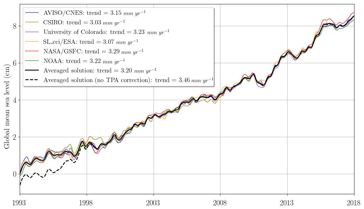
Figure 1Evolution of GMSL time series (corrected for TOPEX-A drift using the Ablain (2017) TOPEX-A correction) from six different groups' (AVISO/CNES, CSIRO, University of Colorado, SL_cci/ESA, NASA/GSFC, NOAA) products. The SL_cci/ESA covers the period from January 1993 to December 2016, while all other products cover the full 25-year period (January 1993 to December 2017). Seasonal (annual and semi-annual) signals have been removed and a 6-month smoothing has been applied. An averaged solution has been computed from the six groups. GMSL time series have the same average on the 1993–2015 period (common period) and the averaged solution starts at zero in 1993. The averaged solution without TOPEX-A correction has also been represented. A GIA correction of −0.3 mm yr−1 has been subtracted from each data set. A correction of +0.10 mm yr−1 due to the deformations of the ocean bottom in response to modern melt of land ice (Frederikse et al., 2017; Lickley et al., 2018) has also been added.
In a previous study, Ablain et al. (2009) have proposed a realistic estimate of the uncertainty in the GMSL trend over 1993–2008, using an approach based on the error budget. They have identified the radiometer wet tropospheric correction as one of the main sources of error. They have also proposed the orbital determination, the inter-calibration of altimeters and the estimate of the altimeter range, sigma-0 and significant wave height (mainly on TOPEX/Poseidon) as significant sources of error. When all the terms were accounted for, they have found that the uncertainty in the trend over 1993–2008 was ±0.6 mm yr−1 within a 90 % confidence level. This is larger than the uncertainty of ±0.3 mm yr−1 over a 10-year period required by GCOS (GCOS, 2011). In the framework of the ESA Sea Level Climate Change Initiative (SL_cci), significant improvements have been obtained estimating the sea level from space (Ablain et al., 2015; Quartly et al., 2017; Legeais et al., 2018) to get closer to the GCOS requirements. New altimeter standards, including new wet troposphere corrections, new orbit solutions, new atmospheric corrections and others, were selected and applied in order to improve the sea-level estimation. The GMSL trend uncertainties were then updated and estimated at different temporal and spatial scales (Ablain et al., 2015; Legeais et al., 2018). During the second altimetry decade (2002–2014), Ablain et al. (2015) have estimated that the uncertainty in the GMSL trend was lower than ±0.5 mm yr−1 within a 90 % confidence level (CL) for periods longer than 10 years.
In previous studies, the uncertainty in GMSL has been assessed for long-term trends (periods of 10 years or more, starting in 1993), inter-annual timescales (between 1 and 5 years) and annual timescales (Ablain et al., 2009, 2015). This estimation of the uncertainty at three timescales is a valuable first step, but it is not enough, as it does not fully meet the needs of the scientific community. In many climatic studies the GMSL uncertainty is required at different timescales and spans within the 25-year altimetry record. In sea-level budget studies based on the evolution of GMSL components, these estimates have been carried out at a monthly timescale. In this way, the GMSL monthly changes have been interpreted in terms of changes in ocean mass (Gravity recovery and climate experiment – GRACE – mission). This is also the case for studies estimating the Earth's energy imbalance with the sea-level budget approach (Meyssignac et al., 2019). In the studies on the detection and the attribution of climate change (e.g. Slangen et al., 2017), the uncertainty in the trend estimates is needed, but over different time spans than those addressed in Ablain et al. (2015, 2009) and in Legeais et al. (2018). The uncertainty in different metrics is often needed. Dieng et al. (2017) and Nerem et al. (2018) have recently estimated the acceleration in the GMSL over 1993–2017, finding a small acceleration (0.08 mm yr−2) over the 25-year long altimetry record.
In this paper we focus on the uncertainty in the GMSL record arising from instrumental errors in the satellite altimetry. The uncertainties of the measurements have been quantified in the GMSL record. This is important information for the studies in detection and attribution of the climatic changes, estimating the GMSL rise as a response to the anthropogenic activity. But this is not sufficient. In the detection–attribution studies the response of the GMSL to the anthropogenic activity needs to be separated from the response to the natural variability of the climate system, representing an additional source of uncertainty.
The objective of this paper is to estimate the error variance–covariance matrix of the GMSL (on a 10 d basis) from satellite altimetry measurements. This error variance–covariance matrix provides a comprehensive description of the uncertainties in the GMSL to users. It covers all timescales that are included in the 25-year long satellite altimetry record: from 10 d (the time resolution of the GMSL time series) to multidecadal timescales. It also enables us to estimate the uncertainty in any metric derived from GMSL measurements such as trend, acceleration or other moments of higher order in a consistent way.
We used an error budget approach to a global scale on a 10 d basis in order to calculate the error variance–covariance matrix. We considered all the major sources of uncertainty in the altimetry measurements, including the wet tropospheric correction, the orbital solutions, and the inter-calibration of satellites. We have also taken into account the time correlation between the different sources of uncertainty (Sect. 2). The errors have been separately characterized for each altimetry mission, since they have been affected by different sources of uncertainty (Sect. 2). On the basis of the error variance–covariance matrix we estimate the uncertainty in GMSL individual measurements on a 10 d basis (Sect. 3) and the uncertainty in trend and acceleration over all periods included in the 25-year satellite altimetry record (1993–2017) (Sect. 4). Note that in this article all uncertainties associated with the GMSL are reported with a 90 % CL unless stated otherwise.
The six main groups that provide satellite-altimetry-based GMSL estimates (AVISO/CNES, SL_cci/ESA, University of Colorado, CSIRO, NASA/GSFC, NOAA) use 1 Hz altimetry measurements from the T/P, Jason-1, Jason-2 and Jason-3 missions from 1993 to 2018 (1993–2015 for SL_cci/ESA). Each group processes the 1 Hz data with geophysical corrections to correct the altimetry measurements for various aliasing, biases and drifts caused by different atmospheric conditions, sea states, ocean tides and others (Ablain et al., 2009). They spatially average the data over each 10 d orbital cycle to provide GMSL time series on a 10 d basis. The differences among the GMSL estimates from several groups arise from data editing, from differences in the geophysical corrections and from differences in the used method to spatially average individual measurements during the orbital cycles (Masters et al., 2012; Henry et al., 2014).
Recently, the comparisons of the GMSL time series derived from satellite altimetry with independent estimates are based on tide gauge records (Valladeau et al., 2012; Watson et al., 2015) or on the combination of the contribution to sea level from thermal expansion, land ice melt and land water storage (Dieng et al., 2017). They have shown that there was a drift in the GMSL record over the period 1993–1998. This drift is caused by an erroneous onboard calibration correction on TOPEX altimeter side-A (denoted TOPEX-A). TOPEX-A was operated from launch in October 1992 to the end of January 1999. Then the TOPEX side-B altimeter (denoted TOPEX-B) took over in February 1999 (Beckley et al., 2017). The impact on the GMSL changes is −1.0 mm yr−1 between January 1993 and July 1995, and +3.0 mm yr−1 between August 1995 and February 1999, with an uncertainty of ±1.7 mm yr−1 (within a 90 % CL, Ablain, 2017).
Without taking into account the TOPEX-A drift correction, the differences between all GMSL time series are small. The maximum trend difference between all time series over 1993–2017 is lower than 0.15 mm yr−1, representing less than 5 % of the GMSL trend. The differences observed at interannual timescales are also small (<2 mm). By correcting the drift of TOPEX-A using either of the available empirical corrections (WCRP Global Sea Level Budget Group, 2018), the differences among solutions remain the same (the difference between empirical corrections being smaller than the difference between the raw GMSL time series). Therefore, the choice of one or the other GMSL record is not decisive in this study, whose purpose is to characterize the uncertainties. Hereafter, we use the GMSL AVISO record. The corresponding altimeter standard corrections and the GMSL processing methods are described on the AVISO website (https://www.aviso.altimetry.fr/msl/, last access: 1 August 2019).
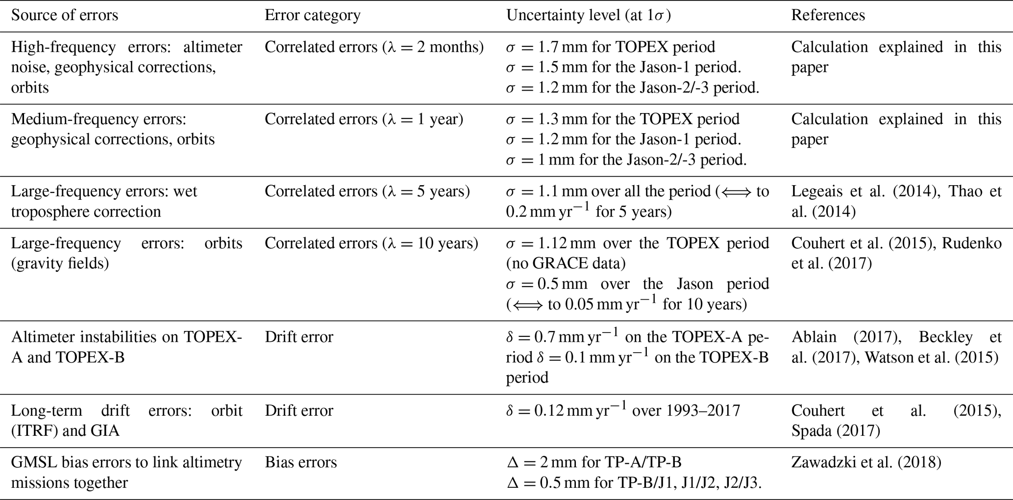
This section describes the different errors that affect the altimetry GMSL record. It builds on the GMSL error budget presented in Ablain et al. (2009) and extends this work by taking into account the new altimeter missions (Jason-2, Jason-3) and the recent findings on altimetry error estimates. Three types of errors are considered: (a) biases in GMSL between successive altimetry missions which are characterized by bias uncertainties (±Δ) at a given time (t); (b) drifts in GMSL characterized by a trend uncertainty (±δ); and (c) other measurement errors which exhibit time correlation (so-called residual time-correlated errors hereafter). The residual time-correlated errors are characterized by their standard deviation (σ) and by the correlation timescale (λ). All altimetry errors identified in this study are summarized in Table 1 and are detailed hereafter. Note that all uncertainties reported in Table 1 are Gaussians, and they are given at the 1-σ level (i.e. we provide the standard deviation of the Gaussian, denoted 1σ hereafter).
The biases can arise between the GMSL record of two successive satellite missions like between T/P and Jason-1 in May 2002, between Jason-1 and Jason-2 in October 2008 and between Jason-2 and Jason-3 in October 2016. These biases are estimated during dedicated 9-month inter-calibration phases when a satellite altimeter and its successor fly over the same track, 1 min apart. During the inter-calibration phases the bias is estimated and corrected for. Different missions show different biases, but the uncertainty in the bias correction is the same for all inter-calibration phases and amounts: ±0.5 mm (Zawadzki and Ablain, 2016). The situation is different for the switch from TOPEX-A to TOPEX-B in February 1999 because it was impossible to do any inter-calibration phase between the two sides of TOPEX (as both instruments were flying on the same spacecraft). For the switch, we assume that the uncertainty in GMSL is larger and is about 2 mm (Zawadzki and Ablain, 2016).
The drifts may occur in the GMSL record because of drifts in the TOPEX-A and TOPEX-B radar instruments, because of drifts in the International Terrestrial Reference Frame (ITRF) realization in which altimeter orbits are determined or because of drifts in the glacial isostatic adjustment (GIA) correction applied to the GMSL record. As explained before, the TOPEX-A record shows a spurious drift due to an erroneous onboard calibration correction of the altimeter (Beckley et al., 2017). This drift has been corrected by using several empirical approaches (Ablain, 2017; Beckley et al., 2017; Dieng et al., 2017) that are all affected by a significant uncertainty. We estimated this uncertainty to be ±0.7 mm yr−1 (1σ level) over the TOPEX-A period (1993–1998), with a comparison against an independent GMSL estimate based on tide gauge records (Ablain, 2017). For the TOPEX-B record, no GMSL drift has been reported, but Ablain et al. (2012) showed significant sigma-0 instabilities of the order of 0.1 dB, which generate through the sea-state bias correction an uncertainty of ±0.1 mm yr−1 (1σ level) in the GMSL record over the TOPEX-B period (February 1999–April 2002). Concerning the ITRF realization, Couhert et al. (2015) have shown that the uncertainty in the ITRF realization drift generates an uncertainty of ±0.1 mm yr−1 (1σ level) in the GMSL trend over 1993–2015. We adopt this value here for the whole period 1993–2017. For the uncertainty in the GIA correction applied to the GMSL, we use the value of 0.05 mm yr−1 (1σ level) over the altimetry period from Spada (2017) (the value is taken from Table 1 in Spada, 2017). It has been confirmed recently with an ensemble of 1000 GIA runs; see Melini and Spada (2019). Combining the uncertainty in the GMSL trend over 1993–2017 from GIA and ITRF and assuming that they are not correlated yields an uncertainty in the GMSL trend of ±0.12 mm yr−1 over 1993–2017 (1σ level). In addition to the GIA correction and the TOPEX correction, we apply an elastic correction to the GMSL record of +0.10 mm yr−1 to account for the elastic deformations of the ocean bottom in response to modern melt of land ice (Frederikse et al., 2017; Lickley et al., 2018). The uncertainty in this correction arises from the uncertainty associated with the computation of the elastic response of the solid Earth (mainly from the uncertainty associated with the procedure to solve the sea-level equation, uncertainty in the choice of the Love numbers, and uncertainty generated by the truncation degree of the spherical harmonics) and the uncertainty in the mass redistributions that cause the elastic deformation. Because the elastic response of the Earth is reasonably well defined (Mitrovica et al., 2011), the uncertainty in the elastic correction is largely dominated by the uncertainty in the mass redistribution (Frederikse et al., 2017). The uncertainty in the mass redistribution is about ±10 % on the current ice mass loss (e.g. Blazquez et al., 2018). It yields an uncertainty of ±10 % in the elastic correction (because the elastic response of the Earth is linear). This uncertainty amounts to ±0.01 mm yr−1, which is very small. It is an order of magnitude smaller than the uncertainty considered in this study (see Table 1). So we neglect this source of uncertainty here.
The residual time-correlated errors are separated into two different groups, depending on their correlation timescales. The first group gathers errors with short correlation timescales, i.e. lower than 2 months and between 2 months and 1 year. The second group gathers errors with long correlation timescales between 5 and 10 years. In the first group the errors are mainly due to the geophysical corrections (ocean tides, atmospheric corrections), to the altimeter corrections (sea-state bias correction, altimeter ionospheric corrections), to the orbital calculation, and to the potential altimeter instabilities (altimeter range and sigma-0 instabilities). At timescales below 1 year, the variability of the corrections' time series is dominated by errors, such that the variance of the error in each correction is estimated by the variance of the correction's time series. For errors with correlation timescales lower than 2 months, we estimated the standard deviation (σ) of the error from the correction's time series filtered with a 2-month high-pass filter. Since the standard deviation of the errors depends on the different altimeter missions, the standard deviation has been separately estimated for each altimeter mission. We find σ=1.7 mm over the T/P period, σ=1.5 mm over the Jason-1 period, and σ=1.2 mm over the Jason-2/-3 period. For errors with a correlation timescale between 2 months and 1 year, we used the same approach and filtered the correction time series with a band-pass filter. In this case we find σ=1.3 mm over the T/P period, σ=1.2 mm over the Jason-1 period, and σ=1.0 mm over the Jason-2/-3 period. Unsurprisingly, the highest errors are obtained for T/P and the lowest ones for Jason-2/-3. This is because of (1) larger altimeter range instabilities in T/P (Ablain et al., 2012; Beckley et al., 2017), (2) the presence of a 59 d signal error in the altimeter range of T/P (Zawadzki et al., 2018), and (3) the deterioration in the performance of atmospheric corrections in the early years of the altimetry era (Legeais et al., 2014). Note that Jason-1 also shows higher errors than Jason-2 and Jason-3 at timescales below 1 year (Couhert et al., 2015).
In the second group of residual time-correlated errors, errors are due to the onboard microwave radiometer calibration, yielding instabilities in the wet troposphere correction, and also due to the orbital calculation (Couhert et al., 2015). Since these errors are correlated at timescales longer than 5 years, they cannot be estimated with the standard deviation of the correction time series, too short (25-year long) to sample the time correlation. For this group of residual time-correlated errors, we used simple models to represent the time correlation of the errors. For the wet troposphere correction, several studies (Legeais et al, 2018) have identified long-term differences among the computed corrections from the different microwave radiometers and from the different atmospheric reanalyses (Dee et al., 2011). These studies report a difference in the wet tropospheric correction for GMSL in the range of ±0.2–0.3 mm yr−1 for periods of 5 to 10 years. Here, we adopt a conservative approach and we model the error in wet tropospheric correction with a correlated error at 5 years with a standard deviation of 1.2 mm (1σ level). The correlation is modelled with a Gaussian attenuation based on the wavelength of the errors: with λ=5 years. In terms of trends, this residual time-correlated error generates an uncertainty of ±0.2 mm yr−1 over 5-year periods. For the error in the orbit calculation, comparisons of different orbit solutions showed differences of ±0.05 mm yr−1 on 10-year timescales due to errors in the modelling of the Earth's time-varying gravity field (Couhert et al., 2015). We model this error with a correlated error at a 10-year timescale with a standard deviation of 0.5 mm (1σ level). The correlation is modelled by the same Gaussian distribution as before with λ=10 years. In terms of trends, it corresponds to an uncertainty of ±0.05 mm yr−1 over 10-year periods.
In the next section these different terms of the GMSL error budget are combined together to build the error variance–covariance matrix. Note that the different terms of the altimeter GMSL error budget described here are based on the current knowledge of altimetry measurement errors. As the altimetry record increases in length with new altimeter missions, the knowledge of the altimetry measurement also increases and the description of the errors improves. This implies that the error variance–covariance matrix is expected to improve and change in the future.
In this section we derived the error variance–covariance matrix (Σ) of the GMSL from the error budget described in Sect. 2. We assumed that all error sources shown in Table 1 are independent of each other. Thus the Σ matrix is the sum of the individual variance–covariance matrix of each error source Σi in the error budget (see Fig. 2). Each Σi matrix is calculated from a large number of random draws (>1000) of the simulated error signal using the model described in Sect. 2 (either a bias, drift or time-correlated signal) fed with a standard normal distribution.
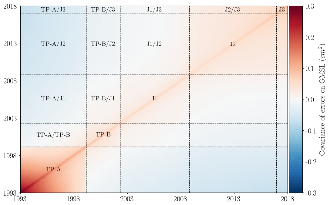
Figure 2Error variance–covariance matrix of altimeter GMSL on the 25-year period (January 1993 to December 2017).
The resulting shape of each individual Σi matrix depends on the type of error (bias, drift or time-correlated signal; see Fig. 2). For the bias, the Σi matrix takes the shape of constant square blocks each side of the time occurrence of the bias correction (see for example the square matrix for TOPEX-A and TOPEX-B in the lower-left corner of Fig. 2 along the diagonal). This square block shape means that the error in the bias correction generates an error on the GMSL which is fully correlated along time before and after the bias correction time, but which is not correlated along time for dates that are apart from the bias correction time. This is consistent with what we expect from a bias correction error. Note that in this article (and in climate change studies in general) we are interested only in GMSL changes, trends or acceleration but not in the mean time GMSL (which is the absolute reference of GMSL). Thus, we have removed from the GMSL time series the temporal mean over 1993–2017. The reference of the GMSL is thus arbitrary and assumed to be perfectly known. This is because the reference of the GMSL is not affected by the biases' correction error here.
For the drifts, the Σi matrix takes the shape of a horse saddle. This is because an error in the GMSL drift over a given period generates errors in the GMSL time series which are correlated when they are close in time and anti-correlated when they are on the opposite side of the drift period.
For residual time-correlated errors, the Σi matrix takes the shape of a diagonal matrix with off-diagonal terms of smaller amplitude. The further from the diagonal the off-diagonal terms are, the more attenuated they are. The attenuation rate is a Gaussian attenuation based on the wavelength of the time-correlated errors (), with various timescales λ.
All individual Σi matrices are summed up together to build the total error variance–covariance matrix Σ of the altimetry-derived continuous GMSL record over 1993–2018 (see Fig. 2). As expected, the dominant terms of the matrix are on the diagonal. They are largely due to the different sources of errors with correlation timescales below 1 year (first group of errors in Sect. 2). The diagonal terms are highest at the beginning of the altimetry period when T/P was at work. This is because of larger altimeter range instabilities in T/P, the presence of a 59 d signal error on the altimeter range of T/P and poorer performance of atmospheric corrections in the early years of the altimetry era (Legeais et al., 2014). The dominant off-diagonal terms are also found during the T/P period (in the lower-left corner of the matrix; see Fig. 2). The terms are induced by the TOPEX-A trend error and the large bias correction uncertainty between TOPEX-A and TOPEX-B (because of the absence of an inter-calibration phase between TOPEX-A and TOPEX-B).
We estimated the GMSL uncertainty envelope from the square root of the diagonal terms of Σ (see Fig. 3). As expected, the GMSL time series shows a larger uncertainty during the T/P period (5 to 8 mm) than during the Jason period (close to 4 mm). The bias correction uncertainty between TOPEX-A and TOPEX-B in February 1999 is also clearly visible, with a 1 mm drop in the uncertainty after the switch to TOPEX side-B. Note that the uncertainty envelope has a parabolic shape and shows smaller uncertainties during the beginning of the Jason-2 period (3.5 mm around 2008) than over the Jason-3 period (4.5 mm). This is not because Jason-1 and Jason-2 errors are smaller than Jason-3's errors. Actually, Jason-2 and Jason-3 errors are slightly smaller than Jason-1 errors thanks to better orbit determination. The uncertainties are smaller during the Jason-1 and Jason-2 periods because this period is in the center of the record. It benefits from prior and posterior data that covariate and help in reducing the uncertainty when they are combined together. In contrast, the Jason-3 period is located at the end of the record and does not benefit from posterior data to help reduce the uncertainty.

Figure 3Evolution in time of GMSL measurement uncertainty within a 90 % confidence level (1.65σ) on the 25-year period (January 1993 to December 2017).
In Fig. 4 we superimposed the GMSL time series (average of the GMSL time series in Fig. 1) and the associated uncertainty envelope. For the TOPEX-A period we tested three different curves with three different corrections based on the removal of the Cal-1 mode (Beckley et al., 2017), based on the comparison with tide gauges (Watson et al., 2015; Ablain, 2017), or based on a sea-level closure budget approach (Dieng et al., 2017). The uncertainty envelope is centred on the corrected record for TOPEX-A drift with the correction based on Ablain et al. (2017). As was expected, all the empirically corrected GMSL records are within the uncertainty envelope.
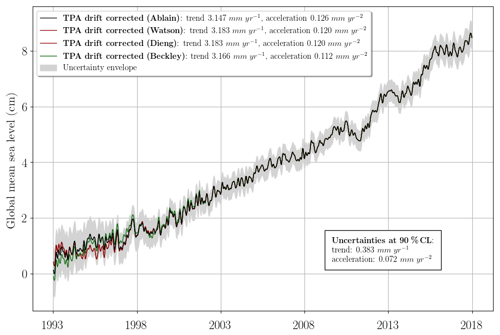
Figure 4Evolution of the AVISO GMSL with different TOPEX-A corrections. On the black, red and green curves, the TOPEX-A drift correction has been, respectively, applied based on Ablain (2017), Watson et al. (2015), Dieng et al. (2017) and Beckley et al. (2017). The uncertainty envelope, as well as the trend and acceleration uncertainties, are given to a 90 % confidence level (1.65σ). Seasonal (annual and semi-annual) signals removed and 6-month smoothing applied. A GIA correction of −0.3 mm yr−1 has been subtracted from each data set. A correction of +0.10 mm yr−1 due to the deformations of the ocean bottom in response to modern melt of land ice (Frederikse et al., 2017; Lickley et al., 2018) has also been added.
The variance–covariance matrix can be used to derive the uncertainty in any metric based on the GMSL time series. In this section we used the error variance–covariance matrix to estimate the uncertainty in the GMSL trend and acceleration over any period of 5 years and more within 1993–2017.
Recently, several studies (Watson et al., 2015; Dieng et al., 2017; Nerem et al., 2018; WCRP Global Sea Level Budget Group, 2018) have found a significant acceleration in the GMSL record from satellite altimetry (after correction for the TOPEX-A drift). The occurrence of an acceleration in the record should not change the estimation of the trend when calculated with a least squared approach. However, it can affect the estimation of the uncertainty in the trend. To cope with this issue, we address here at the same time both the estimation of the trend and acceleration in the GMSL record. In order to obtain this objective, we used a second-order polynomial as a predictor. Considering the GMSL record has n observations, let X be an n×3 predictor where the first column contains only ones (representing the constant term), the second column contains the time vector (representing the linear term) and the third column contains the square of the time vector (representing the squared term). Let y be an n×1 vector of independent observations of the GMSL. Let ϵ be an n×1 vector of disturbances (GMSL non-linear and non-quadratic signals) and errors. Let β be the 3×1 vector of unknown parameters that we want to estimate, namely the GMSL y intercept, the GMSL trend and the GMSL acceleration. Our linear regression model for the estimation of the GMSL trend and acceleration will thus be
with
where Σ is the variance–covariance matrix of the observation errors (estimated in the previous section). Σ is different from the identity because of the correlated noise (see Sect. 2).
The most common method to estimate the GMSL trend and acceleration is the ordinary least squares (OLS) estimator in its classical form (Cazenave and Llovel, 2010; Masters et al., 2012; Dieng et al., 2015; Nerem et al., 2018). This is also the most common method for estimating trends and accelerations in other climate-essential variables (Hartmann, et al., 2014, and references therein). For these reasons, we turn here to the OLS to fit the linear regression model. The estimator of β with the OLS approach, denoted , is
In most cases, ϵ follows a N(0,σ2I) distribution, which implies that follows a normal law:
The issue with this common framework is that the uncertainty in the trend and acceleration estimates does not take into account the correlated errors of the GMSL observations.
To address this issue, we used a more general formalism to integrate the GMSL error into the trend uncertainty estimation, following Ablain et al. (2009), Ribes et al. (2016) and IPCC AR5 (Hartmann, et al., 2014; see in particular Box 2.2 and the Supplement). The OLS estimator is left unchanged (and is still unbiased), but its distribution is revised to account for Σ, leading to
Note that this estimate is known to be less accurate than the general least square estimate (GLS, which is the optimal estimator in the case where Σ≠I) in terms of the mean square error, because its variance is larger. A generalized least square estimate would probably help in narrowing slightly the trend uncertainty, but the difference would likely be small as the GMSL time series is almost linear in time. Important advantages of using OLS here are that (i) OLS is consistent with previous estimators of GMSL trends as well as estimators of trends in other essential climate variables than GMSL (e.g. Hartmann, et al., 2014) and that (ii) the OLS best estimate does not depend on the estimated variance–covariance matrix Σ.
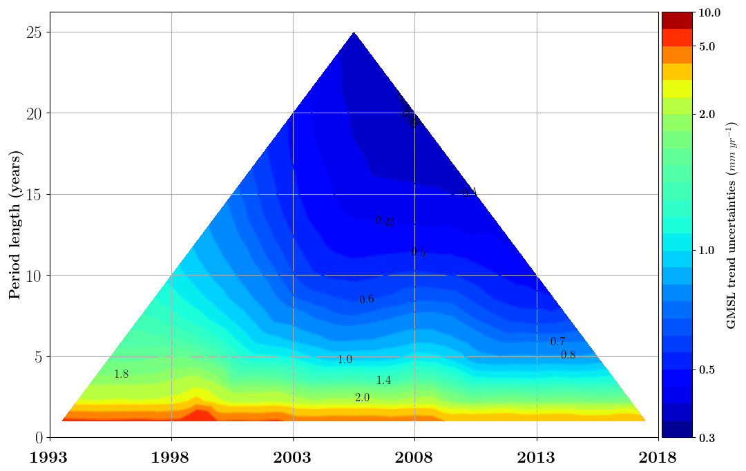
Figure 5GMSL trend uncertainties (mm yr−1) estimated for all altimeter periods within the 25-year period (January 1993 to December 2017). The confidence level is 90 % (1.65σ). Each colored pixel represents, respectively, the half-size of the 90 % confidence range in the GMSL trend. Values are given in mm yr−1. The vertical axis indicates the length of the period (ranging from 1 to 25 years) considered in the computation of the trend, while the horizontal axis indicates the center date of the period (for example, 2000 for the 20-year period 1990–2009).
Based on the matrix Σ defined in the previous section and the OLS solution proposed before, we now estimate the GMSL trend (mm yr−1) and acceleration (mm yr−2) uncertainties for any time span included in the period 1993–2017. Results are synthetically displayed in Fig. 5 for trends and in Fig. 6 for accelerations. In Fig. 5, the top of the triangle indicates that the GMSL trend uncertainty over 1993–2017 is ±0.4 mm yr−1 (CL 90 %) and that the GMSL acceleration uncertainty over the same period is ±0.07 mm yr−2 (CL 90 %, Fig. 6). The GMSL acceleration uncertainty estimate is consistent with results of Watson et al. (2015) on the January 1993 to June 2014 time period, where they find an uncertainty of ±0.058 mm yr−2 at 1σ which corresponds to ±0.096 mm yr−2 at the 90 % confidence level. This is slightly larger than the Nerem et al. (2018) estimate, which is ±0.025 mm yr−2 at the 1σ level on the full 25-year altimetry era, which corresponds to ±0.041 mm yr−2 at the 90 % confidence level. But the Nerem et al. (2018) estimate is likely underestimated as they only consider omission errors. The GMSL acceleration uncertainties have been calculated for all periods of 10 years and more within 1993–2017 (Fig. 6). As expected, uncertainties tend to increase when the period length decreases. At 10 years, the GMSL acceleration uncertainties range from ±0.3 mm yr−2 over the T/P period to ±0.25 mm yr−2 over the Jason period. At 20 years they range between ±0.12 and ±0.08 mm yr−2.
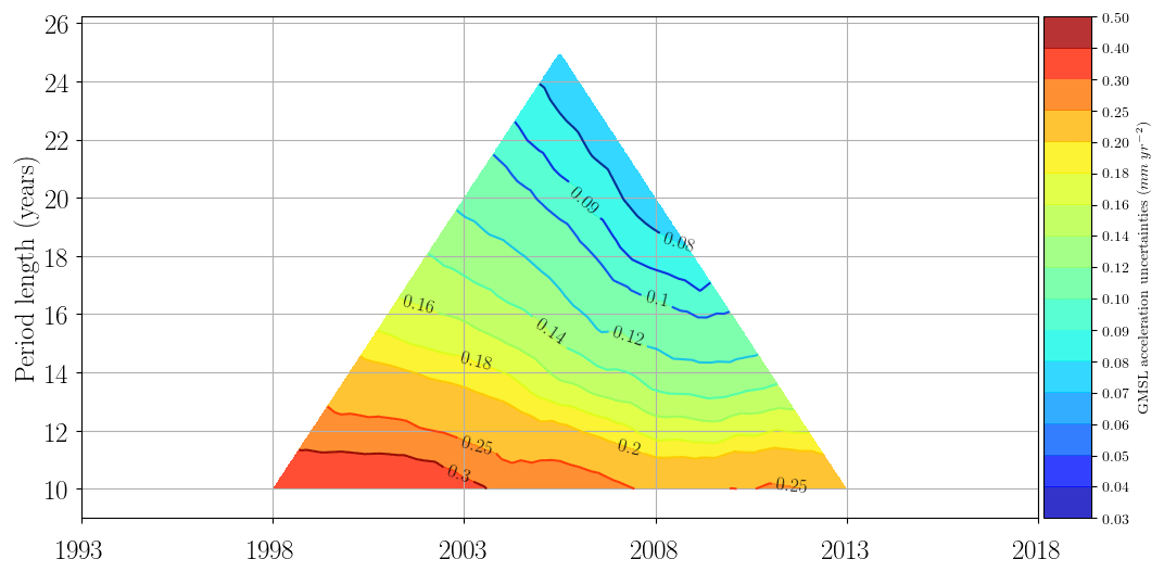
Figure 6GMSL acceleration uncertainties (mm yr−2) estimated for all the altimeter periods within the 25-year period (January 1993 to December 2017). The confidence level is 90 % (1.65σ). Each colored pixel represents, respectively, the half-size of a 90 % confidence range in the GMSL acceleration. Values are given in mm yr−2. The vertical axis indicates the length of the period (ranging from 1 to 25 years) considered in the computation of the acceleration, while the horizontal axis indicates the center date of the period (for example, 2000 for the 20-year period 1990–2009).
A cross-sectional analysis of the 10-year horizontal line in Fig. 5 shows that the GMSL trend uncertainties over 10-year periods decreased from 1.0 mm yr−1 over the first decade to 0.5 mm yr−1 over the last one. The larger uncertainty over the first decade is mainly due to the TOPEX-A drift error, but also due to the large intermission bias uncertainty between TOPEX-A and TOPEX-B, and, to a lesser extent, to the improvement of GMSL accuracy with Jason-2 and Jason-3. Note that the current GCOS requirement of 0.3 mm yr−1 uncertainty over 10 years (GCOS, 2011) is not met at the 90 % confidence level. But the recent record over the last decade based on the Jason series is close to meeting the GCOS requirement, with a 90 % CL.
Figure 5 can also be analysed by following the sides of the triangle. The results of this analysis are plotted in Fig. 7. The plain line corresponds to the left side, read from bottom left to the top of the triangle. The dashed line corresponds to the right side, read from bottom right to the top of the triangle. As expected, both curves show a reduction of the trend uncertainty as the period over which trends are computed increases from 2 to 25 years. The difference between the two lines shows the reduction of GMSL errors thanks to the improvement of the measurement in the latest altimetry missions. The lowest trend uncertainty is obtained with the last 20 years of the GMSL record: 0.35 mm yr−1.
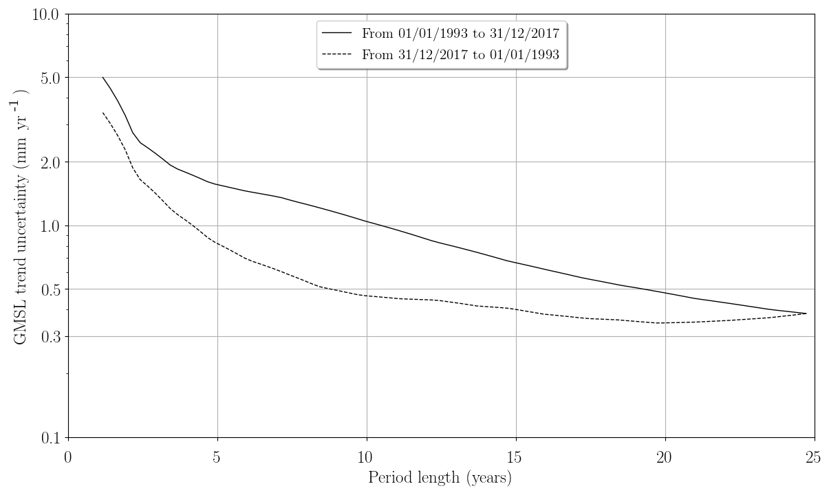
Figure 7Evolution of the GMSL trend uncertainties within a 90 % confidence level (1.65σ) versus the altimeter period length from January 1993 to December 2017 on the plain curve and from December 2017 to January 1993 on the dashed curve.
The periods for which the acceleration in sea level is significant at the 90 % confidence level are shown in Fig. 8. The acceleration is visible at the end of the record for periods of 10 years and longer. The GMSL acceleration is 0.12 mm yr−2 with an uncertainty of 0.07 mm yr−2 at the 90 % confidence level over the 25-year altimetry era. This proves that the acceleration observed in the GMSL evolution is statistically significant. It is worth noting that the different empirical TOPEX-A corrections yield very similar results (0.126 mm yr−2, Ablain, 2017; 0.120 mm yr−2, Dieng et al., 2017; Watson et al., 2015; 0.114 mm yr−2, Beckley et al., 2017). This acceleration at the end of the record is due to an acceleration in the contribution to sea level from Greenland and from other contributions, but to a lesser extent (Chen et al., 2017; Dieng et al., 2017; Nerem et al., 2018). A small acceleration is also visible during the 1993–2005 period at the beginning of the record. This acceleration is likely due to the recovery from the Mount Pinatubo eruption in 1991 (Fasullo et al., 2016). Indeed, Church et al. (2005) showed that the impact of large volcanic eruptions on global ocean heat content is characterized by a rapid reduction in global ocean heat content during the year following the eruption followed by a period of recovery of a few years when global ocean heat content increases faster than before the eruption (see also Gregory et al., 2006, and Delworth et al., 2005). The sea-level record starts in October 1992, which is 1.5 years after the eruption of Mount Pinatubo (15 June 1991). At that time the global ocean heat content was starting to recover with an increasing rate of rise (see Fasullo et al., 2016, their Fig. 2) leading to an acceleration in sea level.
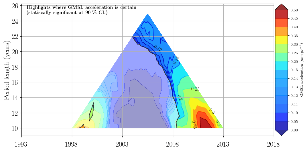
Figure 8GMSL acceleration using the AVISO GMSL time series corrected for the TOPEX-A drift using the correction proposed by Ablain (2017): the acceleration in the shaded areas is not significant (lower than the acceleration uncertainties at the 90 % confidence level). The length of the window (in years) is represented on the vertical axis and the central date of the used window (in years) is represented on the horizontal axis.

Figure 9GMSL trends using the AVISO GMSL time series corrected for the TOPEX-A drift using the correction proposed by Ablain (2017). The length of the window (in years) is represented on the vertical axis and the central date of the window used (in years) is represented on the horizontal axis. A GIA correction of −0.3 mm yr−1 has been subtracted. A correction of +0.10 mm yr−1 due to the deformations of the ocean bottom in response to modern melt of land ice (Frederikse et al., 2017; Lickley et al., 2018) has also been added.
The period for which the trend in sea level is significant at the 90 % confidence level is shown in Fig. 9. In periods when the acceleration is not significant, the second-order polynomial that we used as a predictor to estimate the trend and the acceleration does not hold anymore in principle. For these periods, we should turn out a first-order polynomial. The use of a first-order polynomial does not affect the trend estimates, but only the trend uncertainty estimates. We checked for differences in trend uncertainty when using either second-order or first-order polynomial predictors. We found that these differences are negligible (not shown).
Figure 9 indicates that for periods of 5 years and longer, the trend in GMSL is always significant at the 90 % CL over the whole record. At the end of the record the trend tends to increase. This is consistent with the acceleration plot in Fig. 6. Over the 25 years of satellite altimetry, we find a sea-level rise of 3.35±0.4 mm yr−1 (90 % CL) after correcting for the TOPEX-A GMSL drift. The differences due to the different TOPEX-A corrections are negligible (<0.05 mm yr−1).
The global mean sea-level error variance–covariance matrix is available online at https://doi.org/10.17882/58344 (Ablain et al., 2018).
In this study we have estimated the full GMSL error variance–covariance matrix over the satellite altimetry period. The matrix is available online (see Sect. 7). It provides users with a comprehensive description of the GMSL errors over the altimetry period. This matrix is based on the current knowledge of altimetry measurement errors. As the altimetry record increases in length with new altimeter missions, the knowledge of the altimetry measurement also increases and the description of the errors improves. Consequently, the error variance–covariance matrix is expected to change and improve in the future – hopefully with a reduction of measurement uncertainty in new products.
The uncertainty in the GMSL computed here shows the reliability of altimetry measurements in order to accurately describe the evolution of the GMSL on all timescales from 10 d to 25 years. It also shows the reliability of altimetry measurements in order to estimate the trends and accelerations of the sea level. Along the altimetry record, we find that the uncertainty in each individual GMSL measurement decreases with time. It is smaller during the Jason era (2002–2018) than during the T/P period (1993–2002). Over the entire altimetry record, 1993–2017, we estimate the GMSL trend to 3.35±0.4 mm yr−1 (90 % CL, after correcting the TOPEX-A GMSL drift). We also detect a significant GMSL acceleration over the 25-year period at 0.12±0.07 mm yr−2 (90 % CL).
In this study, several assumptions have been made that could be improved in the future. Firstly, the modelling of altimeter errors should be regularly revisited and improved to consider a better knowledge of errors (e.g. stability of wet troposphere corrections) and to consider future altimeter missions (e.g. Sentinel-3 and Sentinel-6 missions). Concealing the mathematical formalism, the OLS method has been applied because it is the most common approach used in the climate community to calculate trends in any climate data records. However, this is not the optimal linear estimator. The use of a generalized least square approach should involve some narrowing of trend or acceleration uncertainty. Another topic of concern is the consideration of the internal and forced variability of the GMSL. Here we only considered the uncertainty in the GMSL due to the satellite altimeter instrument. In a future study, it would be interesting to consider the partitioning of the GMSL into the forced response to anthropogenic forcing and the natural response to natural forcing and to the internal variability. Estimating the natural GMSL variability (e.g. using models) and considering it to be an additional residual time-correlated error would allow us to calculate the GMSL trend and acceleration representing the long-term evolution of GMSL in relation to anthropogenic climate change.
MA and BM led the study, developed the theory, and wrote the manuscript with input from all the authors. LZ and RJ contributed to the theory and performed the computations. AR contributed to the statistical methodology developed in this paper. GS supervised the part related to the GIA uncertainties. JB, AC, and NP discussed the results. All the authors contributed to the final manuscript.
The authors declare that they have no conflict of interest.
We would like to thank all contributors of the Sea Level CCI (SL_cci) project (Climate Change Initiative programme) and of the SALP (Service d'Altimétrie et de Localisation Précise), with special recognition to Thierry Guinle, SALP project manager at the CNES.
This research has been supported by the ESA in the framework of the Sea Level CCI (SL_cci) project (Climate Change Initiative programme) supported by the CNES in the framework of the SALP (Service d'Altimétrie et de Localisation Précise). Giorgio Spada is funded by a FFABR (Finanziamento delle Attività Base di Ricerca) grant of the MIUR (Ministero dell'Istruzione, dell'Università e della Ricerca) and by a DiSPeA (Dipartimento di Scienze Pure e Applicate of the Urbino 65 University) grant.
This paper was edited by Giuseppe M. R. Manzella and reviewed by two anonymous referees.
Ablain, M.: The TOPEX-A Drift and Impacts on GMSL Time Series, available at: https://meetings.aviso.altimetry.fr/fileadmin/user_upload/tx_ausyclsseminar/files/Poster_OSTST17_GMSL_Drift_TOPEX-A.pdf, Miami, US (October, 2017), available at: https://meetings.aviso.altimetry.fr/fileadmin/user_upload/tx_ausyclsseminar/files/Poster_OSTST17_GMSL_Drift_TOPEX-A.pdf (last access: 8 November 2018), 2017.
Ablain, M., Cazenave, A., Valladeau, G., and Guinehut, S.: A new assessment of the error budget of global mean sea level rate estimated by satellite altimetry over 1993–2008, Ocean Sci., 5, 193–201, https://doi.org/10.5194/os-5-193-2009, 2009.
Ablain, M., Philipps, S., Urvoy, M., Tran, N., and Picot, N.: Detection of Long-Term Instabilities on Altimeter Backscatter Coefficient Thanks to Wind Speed Data Comparisons from Altimeters and Models, Mar. Geod., 35 (Suppl. 1), 258–275, https://doi.org/10.1080/01490419.2012.718675, 2012.
Ablain, M., Cazenave, A., Larnicol, G., Balmaseda, M., Cipollini, P., Faugère, Y., Fernandes, M. J., Henry, O., Johannessen, J. A., Knudsen, P., Andersen, O., Legeais, J., Meyssignac, B., Picot, N., Roca, M., Rudenko, S., Scharffenberg, M. G., Stammer, D., Timms, G., and Benveniste, J.: Improved sea level record over the satellite altimetry era (1993–2010) from the Climate Change Initiative project, Ocean Sci., 11, 67–82, https://doi.org/10.5194/os-11-67-2015, 2015.
Ablain, M., Legeais, J. F., Prandi, P., Marcos, M., Fenoglio-Marc, L., Dieng, H. B., Benveniste, J., and Cazenave, A.: Satellite Altimetry-Based Sea Level at Global and Regional Scales, Surv. Geophys., 38, 7–31, https://doi.org/10.1007/s10712-016-9389-8, 2017.
Ablain, M., Meyssignac, B., Zawadzki, L., Jugier, R., Ribes, A., Cazenave, A., and Picot, N.: Error variance-covariance matrix of global mean sea level estimated from satellite altimetry (TOPEX, Jason 1, Jason 2, Jason 3), https://doi.org/10.17882/58344, 2018.
Beckley, B. D., Callahan, P. S., Hancock, D. W., Mitchum, G. T., and Ray, R. D.: On the “Cal-Mode” Correction to TOPEX Satellite Altimetry and Its Effect on the Global Mean Sea Level Time Series, J. Geophys. Res.-Oceans, 122, 8371–8384, https://doi.org/10.1002/2017JC013090, 2017.
Blazquez, A., Meyssignac, B., Lemoine, J., Berthier, E., Ribes, A., and Cazenave, A.: Exploring the uncertainty in GRACE estimates of the mass redistributions at the Earth surface: implications for the global water and sea level budgets, Geophys. J. Int., 215, 415–430, https://doi.org/10.1093/gji/ggy293, 2018.
Cazenave, A. and Llovel, W.: Contemporary Sea Level Rise, Annu. Rev. Mar. Sci., 2, 145–173, https://doi.org/10.1146/annurev-marine-120308-081105, 2010.
Chen, X., Zhang, X., Church, J. A., Watson, C. S., King, M. A., Monselesan, D., Legresy, B., and Harig, C.: The increasing rate of global mean sea-level rise during 1993–2014, Nat. Clim. Change, 7, 492–495, https://doi.org/10.1038/nclimate3325, 2017.
Church, J. A., White, N. J., and Arblaster, J. M.: Significant decadal-scale impact of volcanic eruptions on sea level and ocean heat content, Nature, 438, 74–77, https://doi.org/10.1038/nature04237, 2005.
Couhert, A., Cerri, L., Legeais, J.-F., Ablain, M., Zelensky, N. P., Haines, B. J., Lemoine, F. G., Bertiger, W. I., Desai, S. D., and Otten, M.: Towards the 1 mm/y stability of the radial orbit error at regional scales, Adv. Space Res., 55, 2–23, https://doi.org/10.1016/j.asr.2014.06.041, 2015.
Dee, D. P., Uppala, S. M., Simmons, A. J., Berrisford, P., Poli, P., Kobayashi, S., Andrae, U., Balmaseda, M. A., Balsamo, G., Bauer, P., Bechtold, P., Beljaars, A. C. M., van de Berg, L., Bidlot, J., Bormann, N., Delsol, C., Dragani, R., Fuentes, M., Geer, A. J., Haimberger, L., Healy, S. B., Hersbach, H., Hólm, E. V., Isaksen, L., Kållberg, P., Köhler, M., Matricardi, M., McNally, A. P., Monge-Sanz, B. M., Morcrette, J.-J., Park, B.-K., Peubey, C., de Rosnay, P., Tavolato, C., Thépaut, J.-N., and Vitart, F.: The ERA-Interim reanalysis: configuration and performance of the data assimilation system, Q. J. Roy. Meteor. Soc., 137, 553–597, https://doi.org/10.1002/qj.828, 2011.
Delworth, T. L., Ramaswamy, V., and Stenchikov, G. L.: The impact of aerosols on simulated ocean temperature and heat content in the 20th century, Geophys. Res. Lett., 32, L24709, https://doi.org/10.1029/2005GL024457, 2005.
Dieng, H. B., Cazenave, A., von Schuckmann, K., Ablain, M., and Meyssignac, B.: Sea level budget over 2005–2013: missing contributions and data errors, Ocean Sci., 11, 789–802, https://doi.org/10.5194/os-11-789-2015, 2015.
Dieng, H. B., Cazenave, A., Meyssignac, B., and Ablain, M.: New estimate of the current rate of sea level rise from a sea level budget approach, Geophys. Res. Lett., 44, 3744–3751, https://doi.org/10.1002/2017GL073308, 2017.
Fasullo, J. T., Nerem, R. S., and Hamlington, B.: Is the detection of accelerated sea level rise imminent?, Sci. Rep., 6, 31245, https://doi.org/10.1038/srep31245, 2016.
Frederikse, T., Riva, R. E. M., and King, M. A.: Ocean Bottom Deformation Due To Present-Day Mass Redistribution and Its Impact on Sea Level Observations: ocean bottom deformation and sea level, Geophys. Res. Lett., 44, 12306–12314, https://doi.org/10.1002/2017GL075419, 2017.
GCOS: Systematic Observation Requirements for Satellite-Based Data Products for Climate (2011 Update) – Supplemental details to the satellite-based component of the “Implementation Plan for the Global Observing System for Climate in Support of the UNFCCC (2010 Update), WMO, 2011.
Gregory, J. M., Lowe, J. A., and Tett, S. F. B.: Simulated Global-Mean Sea Level Changes over the Last Half-Millennium, J. Climate, 19, 4576–4591, https://doi.org/10.1175/JCLI3881.1, 2006.
Hartmann, D. L., Klein Tank, A. M. G., Rusticucci, M., Alexander, L. V., Brönnimann, S., Charabi, Y. A. R., and Zhai, P.: Observations: Atmosphere and Surface, in Climate Change 2013 – The Physical Science Basis?: Working Group I Contribution to the Fifth Assessment Report of the Intergovernmental Panel on Climate Change, Cambridge University Press, Cambridge, 159–254, 2014.
Henry, O., Ablain, M., Meyssignac, B., Cazenave, A., Masters, D., Nerem, S., and Garric, G.: Effect of the processing methodology on satellite altimetry-based global mean sea level rise over the Jason-1 operating period, J. Geodesy, 88, 351–361, https://doi.org/10.1007/s00190-013-0687-3, 2014.
Legeais, J.-F., Ablain, M., and Thao, S.: Evaluation of wet troposphere path delays from atmospheric reanalyses and radiometers and their impact on the altimeter sea level, Ocean Sci., 10, 893–905, https://doi.org/10.5194/os-10-893-2014, 2014.
Legeais, J.-F., Ablain, M., Zawadzki, L., Zuo, H., Johannessen, J. A., Scharffenberg, M. G., Fenoglio-Marc, L., Fernandes, M. J., Andersen, O. B., Rudenko, S., Cipollini, P., Quartly, G. D., Passaro, M., Cazenave, A., and Benveniste, J.: An improved and homogeneous altimeter sea level record from the ESA Climate Change Initiative, Earth Syst. Sci. Data, 10, 281–301, https://doi.org/10.5194/essd-10-281-2018, 2018.
Lickley, M. J., Hay, C. C., Tamisiea, M. E., and Mitrovica, J. X.: Bias in Estimates of Global Mean Sea Level Change Inferred from Satellite Altimetry, J. Climate, 31, 5263–5271, https://doi.org/10.1175/JCLI-D-18-0024.1, 2018.
Masters, D., Nerem, R. S., Choe, C., Leuliette, E., Beckley, B., White, N., and Ablain, M.: Comparison of Global Mean Sea Level Time Series from TOPEX/Poseidon, Jason-1, and Jason-2, Mar. Geod., 35 (Suppl. 1), 20–41, https://doi.org/10.1080/01490419.2012.717862, 2012.
Melini, D. and Spada, G.: Some remarks on Glacial Isostatic Adjustment modelling uncertainties, Geophys. J. Int, 218, 401–413, https://doi.org/10.1093/gji/ggz158, 2019.
Meyssignac, B., Boyer, T., Zhao, Z., Hakuba, M. Z., Landerer, F. W., Stammer, D., Kato, S., Köhl, A., Ablain, M., Abraham, J. P., Blazquez, A., Cazenave, A., Church, J. A., Rebecca, C., Cheng, L., Domingues, C., and Giglio, D.: Measuring Global Ocean Heat Content to estimate the Earth Energy Imbalance, Front. Mar. Sci.-Ocean Observation, in press, 2019.
Mitrovica, J. X., Gomez, N., Morrow, E., Hay, C., Latychev, K., and Tamisiea, M. E.: On the robustness of predictions of sea level fingerprints: On predictions of sea-level fingerprints, Geophys. J. Int., 187, 729–742, https://doi.org/10.1111/j.1365-246X.2011.05090.x, 2011.
Nerem, R. S., Beckley, B. D., Fasullo, J. T., Hamlington, B. D., Masters, D., and Mitchum, G. T.: Climate-change–driven accelerated sea-level rise detected in the altimeter era, P. Natl. Acad. Sci. USA, 115, 2022–2025, https://doi.org/10.1073/pnas.1717312115, 2018.
Quartly, G. D., Legeais, J.-F., Ablain, M., Zawadzki, L., Fernandes, M. J., Rudenko, S., Carrère, L., García, P. N., Cipollini, P., Andersen, O. B., Poisson, J.-C., Mbajon Njiche, S., Cazenave, A., and Benveniste, J.: A new phase in the production of quality-controlled sea level data, Earth Syst. Sci. Data, 9, 557–572, https://doi.org/10.5194/essd-9-557-2017, 2017.
Ribes, A., Corre, L., Gibelin, A.-L., and Dubuisson, B.: Issues in estimating observed change at the local scale – a case study: the recent warming over France: estimating observed warming at the local scale, International J. Climatol., 36, 3794–3806, https://doi.org/10.1002/joc.4593, 2016.
Rudenko, S., Neumayer, K.-H., Dettmering, D., Esselborn, S., Schone, T., and Raimondo, J.-C.: Improvements in Precise Orbits of Altimetry Satellites and Their Impact on Mean Sea Level Monitoring, IEEE T. Geoscience Remote, 55, 3382–3395, https://doi.org/10.1109/TGRS.2017.2670061, 2017.
Slangen, A. B. A., Adloff, F., Jevrejeva, S., Leclercq, P. W., Marzeion, B., Wada, Y., and Winkelmann, R.: A Review of Recent Updates of Sea-Level Projections at Global and Regional Scales, Surv. Geophys., 38, 385–406, https://doi.org/10.1007/s10712-016-9374-2, 2017.
Spada, G.: Glacial Isostatic Adjustment and Contemporary Sea Level Rise: An Overview, Surv. Geophys., 38, 153–185, https://doi.org/10.1007/s10712-016-9379-x, 2017.
Thao, S., Eymard, L., Obligis, E., and Picard, B.: Trend and Variability of the Atmospheric Water Vapor: A Mean Sea Level Issue, J. Atmos. Ocean. Tech., 31, 1881–1901, https://doi.org/10.1175/JTECH-D-13-00157.1, 2014.
Valladeau, G., Legeais, J. F., Ablain, M., Guinehut, S., and Picot, N.: Comparing Altimetry with Tide Gauges and Argo Profiling Floats for Data Quality Assessment and Mean Sea Level Studies, Mar. Geod., 35 (Suppl. 1), 42–60, https://doi.org/10.1080/01490419.2012.718226, 2012.
Watson, C. S., White, N. J., Church, J. A., King, M. A., Burgette, R. J., and Legresy, B.: Unabated global mean sea-level rise over the satellite altimeter era, Nat. Clim. Change, 5, 565–568, https://doi.org/10.1038/nclimate2635, 2015.
WCRP Global Sea Level Budget Group: Global sea-level budget 1993–present, Earth Syst. Sci. Data, 10, 1551–1590, https://doi.org/10.5194/essd-10-1551-2018, 2018.
Zawadzki, L. and Ablain, M.: Accuracy of the mean sea level continuous record with future altimetric missions: Jason-3 vs. Sentinel-3a, Ocean Sci., 12, 9–18, https://doi.org/10.5194/os-12-9-2016, 2016.
Zawadzki, L., Ablain, M., Carrere, L., Ray, R. D., Zelensky, N. P., Lyard, F., Guillot, A., and Picot, N.: Investigating the 59-Day Error Signal in the Mean Sea Level Derived From TOPEX/Poseidon, Jason-1, and Jason-2 Data With FES and GOT Ocean Tide Models, IEEE T. Geosci. Remote, 56, 3244–3255, https://doi.org/10.1109/TGRS.2018.2796630, 2018.
- Abstract
- Introduction
- GMSL data series
- Altimetry GMSL error budget
- The GMSL error variance–covariance matrix
- GMSL uncertainty envelope
- Uncertainty in GMSL trend and acceleration
- Data availability
- Conclusions
- Author contributions
- Competing interests
- Acknowledgements
- Financial support
- Review statement
- References