the Creative Commons Attribution 4.0 License.
the Creative Commons Attribution 4.0 License.
 | 21 Aug 2019
A machine-learning-based global sea-surface iodide distribution
Rosie J. Chance
Liselotte Tinel
Daniel Ellis
Mat J. Evans
Lucy J. Carpenter
Iodide in the sea-surface plays an important role in the Earth system. It modulates the oxidising capacity of the troposphere and provides iodine to terrestrial ecosystems. However, our understanding of its distribution is limited due to a paucity of observations. Previous efforts to generate global distributions have generally fitted sea-surface iodide observations to relatively simple functions using proxies for iodide such as nitrate and sea-surface temperature. This approach fails to account for coastal influences and variation in the bio-geochemical environment. Here we use a machine learning regression approach (random forest regression) to generate a high-resolution (, ), monthly dataset of present-day global sea-surface iodide. We use a compilation of iodide observations (1967–2018) that has a 45 % larger sample size than has been used previously as the dependent variable and co-located ancillary parameters (temperature, nitrate, phosphate, salinity, shortwave radiation, topographic depth, mixed layer depth, and chlorophyll a) from global climatologies as the independent variables. We investigate the regression models generated using different combinations of ancillary parameters and select the 10 best-performing models to be included in an ensemble prediction. We then use this ensemble of models, combined with global fields of the ancillary parameters, to predict new high-resolution monthly global sea-surface iodide fields representing the present day. Sea-surface temperature is the most important variable in all 10 models. We estimate a global average sea-surface iodide concentration of 106 nM (with an uncertainty of ∼20 %), which is within the range of previous estimates (60–130 nM). Similar to previous work, higher concentrations are predicted for the tropics than for the extra-tropics. Unlike the previous parameterisations, higher concentrations are also predicted for shallow areas such as coastal regions and the South China Sea. Compared to previous work, the new parameterisation better captures observed variability. The iodide concentrations calculated here are significantly higher (40 % on a global basis) than the commonly used MacDonald et al. (2014) parameterisation, with implications for our understanding of iodine in the atmosphere. We envisage these fields could be used to represent present-day sea-surface iodide concentrations, in applications such as climate and air-quality modelling. The global iodide dataset is made freely available to the community (https://doi.org/10/gfv5v3, Sherwen et al., 2019), and as new observations are made, we will update the global dataset through a “living data” model.


Iodine in seawater exists in two major forms, iodide (I−) and iodate (). Total inorganic iodine () remains approximately constant across most of the oceans, but the ratio of iodide to iodate varies. Chance et al. (2014) have shown that the ratio will vary with latitude, depth, and oxygen level. A small amount of iodine (<10 %) is thought to be present in organic forms in the open ocean (e.g. Wong, 1991); however, this may be a larger fraction in coastal waters (e.g. Wong and Cheng, 1998). The processes controlling the distribution of the ratio between iodide and iodate remain poorly understood (Chance et al., 2014).
A reason for gaps in our understanding is that the observational dataset of iodide and iodate remains relatively sparse (Chance et al., 2014, 2019a). Despite this paucity in observations, iodine's role in the Earth system has driven multidisciplinary interest in the distribution of iodine compounds in seawater from a number of different research communities, including paleoceanography (e.g. Lu et al., 2016, 2018; Zhou et al., 2015), atmospheric composition (e.g. Ganzeveld et al., 2009; Saiz-Lopez et al., 2014; Sherwen et al., 2016a), and air-quality prediction (e.g. Luhar et al., 2017, 2018; Sarwar et al., 2015; Sherwen et al., 2017b).
The atmospheric science community has seen a particularly large growth in interest in iodine chemistry in the atmosphere and at the sea-surface, as sea-surface I− is believed to be the main driver of atmospheric iodine emissions. The reaction of I− with ozone in the sea-surface micro-layer removes ozone from the atmosphere (dry deposition) (Ganzeveld et al., 2009) and results in the emission of inorganic iodine (HOI and I2) into the atmosphere (Carpenter et al., 2013), which can subsequently catalytically destroy ozone (Chameides and Davis, 1980). Models have shown this can then lead to a feedback mechanism between the increased ozone from pre-industrial and present day, counteracting human-driven increases in tropospheric ozone (Prados-Roman et al., 2015; Sherwen et al., 2017a). A number of model studies have discussed the impact of ocean-sourced iodine on atmosphere composition in the context of air quality (Gantt et al., 2017; Sarwar et al., 2016; Sherwen et al., 2017b), climate (Sherwen et al., 2017b; Saiz-Lopez et al., 2012), aerosols (Sherwen et al., 2017a), and stratospheric ozone (Saiz-Lopez et al., 2015). These atmospheric modelling studies have used relatively simple parameterisations for predictions of sea-surface iodide.
Early parameterisations for sea-surface iodide were based on limited datasets and used either an observed range of iodide concentrations (Coleman et al., 2010; Chang et al., 2004) or a reported relationship with biogeochemical parameters (e.g. chlorophyll in Oh et al., 2008, or nitrate Ganzeveld et al., 2009). However, more recent attempts (Chance et al., 2014; MacDonald et al., 2014) have focused on using correlation analysis to fit compilations of observed iodide concentrations to a variety of commonly measured sea-surface variables, notably sea-surface temperature, but also chlorophyll, salinity, and nitrate. A summary of parameterisations that have been used in previous studies is given in Appendix Table A1. Compilation of all available observations confirmed a strong latitudinal gradient and identified sea-surface temperature as the strongest single predictor of iodide concentration (Chance et al., 2014). This approach has led to Eq. (1) from Chance et al. (2014) and Eq. (2) from MacDonald et al. (2014).
Figure 1 shows the global annual mean distribution of sea-surface iodide calculated using these parameterisations (Eqs. 1 and 2) and sea-surface temperature fields (Locarnini et al., 2013). Although both equations predict a similar distribution (higher concentrations in tropical waters and lower in polar waters), Eq. (1) generally predicts iodide concentrations 2–4 times higher than Eq. (2). In developing Eq. (1), Chance et al. (2014) compiled iodide observations from both coastal and non-coastal sites. However, Eq. (2) used a relatively small subset (14 %) of these observations, which did not include coastal sites, which may explain the lower concentrations. Equation (2) also has an Arrhenius form, which could be interpreted to suggest that iodide concentrations are controlled by abiotic reaction kinetics. However, this has not been demonstrated, and Chance et al. (2014) discussed how microbiological activity and oceanic mixing are currently thought to be the primary controls. The choice of parameterisation (Eq. 2 versus Eq. 1) results in a difference of 50 % in the calculated global emissions of iodine into the atmosphere (Sherwen et al., 2016a).
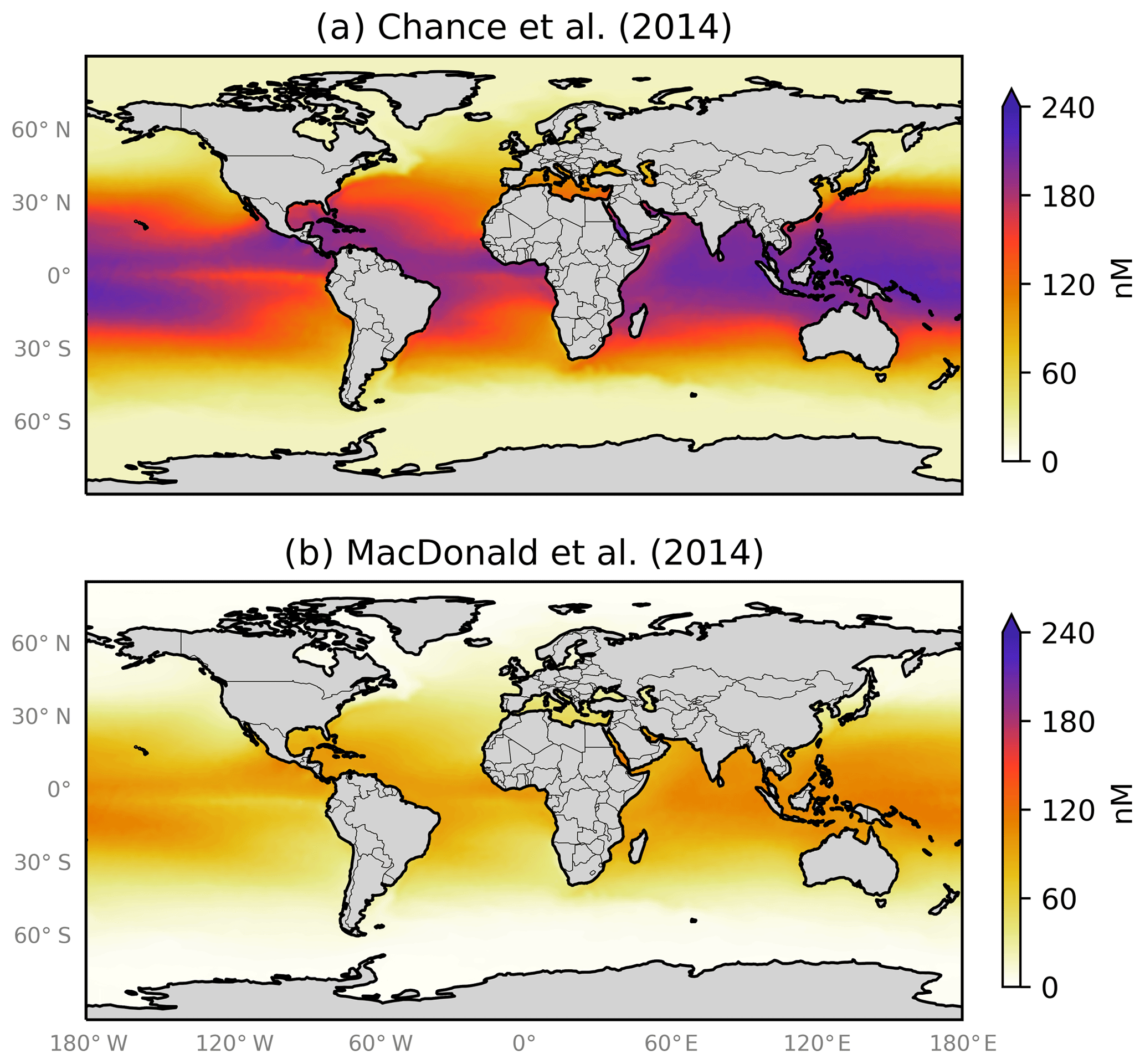
Figure 1Annual average sea-surface iodide concentrations predicted by (a) Eq. (1) from Chance et al. (2014) and (b) Eq. (2) from MacDonald et al. (2014). Temperature fields used to make spatial predictions were from the World Ocean Atlas (Locarnini et al., 2013). Earth raster and vector map data used are freely available from Natural Earth (http://www.naturalearthdata.com/, last access: 23 July 2019).
Table 1Ancillary variables extracted onto a global () grid on a monthly basis.
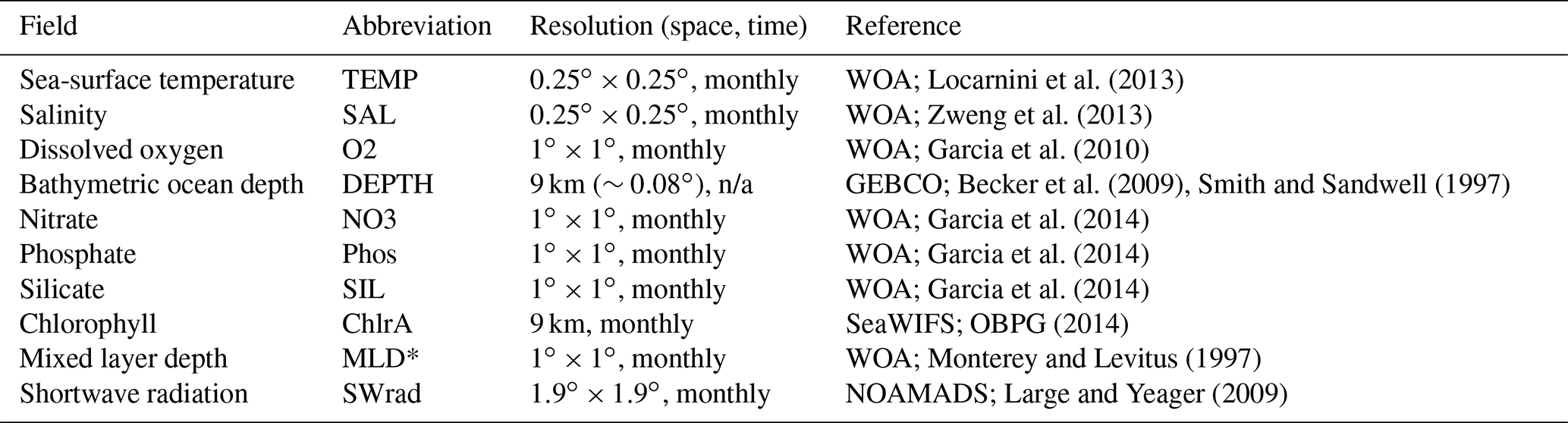
Expansion of Acronyms. WOA: World Ocean Atlas, SeaWIFS: Sea-Viewing Wide Field-of-View Sensor, GEBCO: General Bathymetric Chart of the Oceans, NOAMADS: NOAA National Operational Model Archive and Distribution System. (*) Three available mixed layer depth (MLD) definitions in WOA (vd: variable potential density, pt: potential temperature, pd: potential density) were processed from comma-separated value (CSV) to NetCDF files and extracted. Following Chance et al. (2014), the monthly sum and maximum MLD was also computed (vd, pt, pd) and used for building predictions of iodide. When just the variable MLD is shown, it is MLD as defined by potential temperature. n/a – not applicable
Considering the need for spatially resolved sea-surface iodide fields by models and the paucity of observations, parameterisations are required that can yield predictions from ancillary variables. This is a regression problem and a number of approaches are available. Conventional linear and linear multi-variant approaches have been used in the past (e.g. see summary in Appendix Table A1). However, they need to assume a functional relationship between the dependent and independent variables. Another approach is machine learning, which uses algorithms to build predictive models. These algorithms take a different approach and use a non-parametric formulation. Machine learning approaches range from interpretable options such as the random forest algorithm (Breiman, 2001) to less interpretable ones such as artificial neural networks (Gardner and Dorling, 1998). On the more interpretable end, machine learning algorithms are being used increasingly within environmental sciences, with recent examples including linear ridge regression and random forest models to replace computationally expensive processes (Keller and Evans, 2019; Nowack et al., 2018) and Gaussian process emulation to explore model biases on a global scale (Lee et al., 2011; Revell et al., 2018).
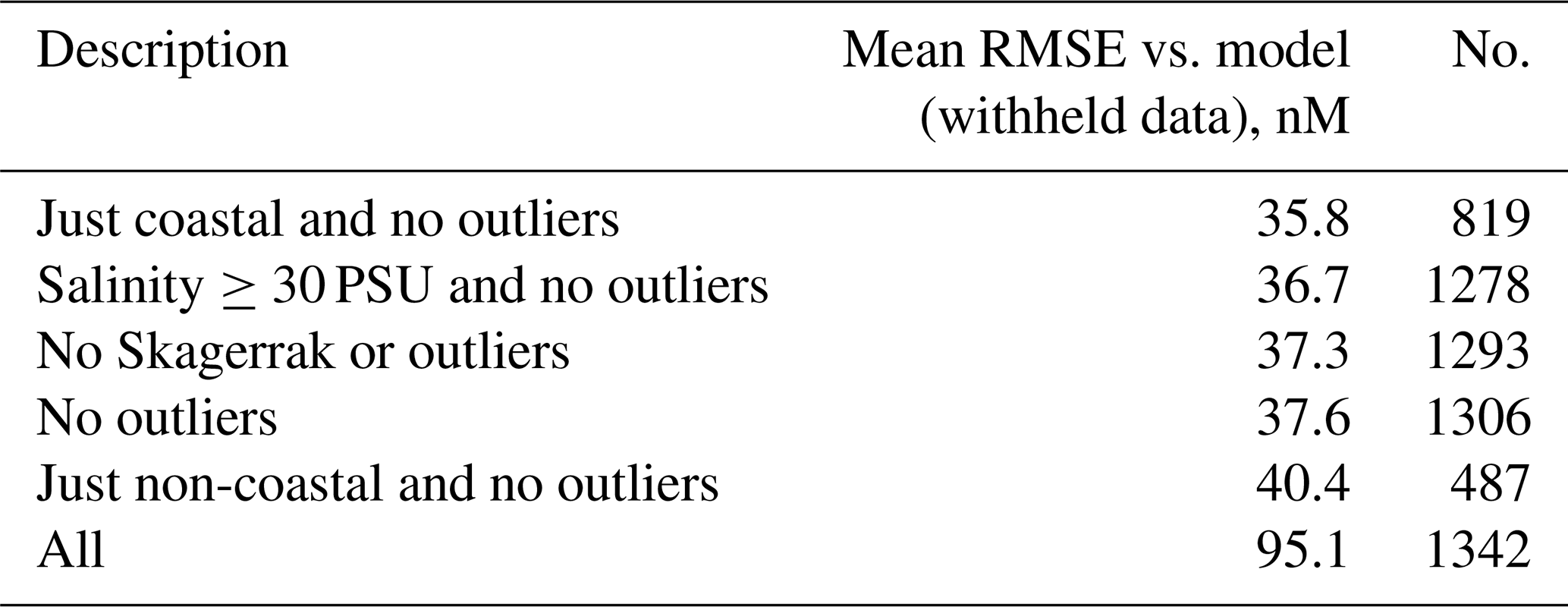
Table 2Splits of dataset used to evaluate outliers and their performance against the withheld data. The root mean square error (RMSE) statistic given as the mean of the performance against the withheld data for 20 different models built from 20 different pseudo-random initialisations (Sect. 3.2). The model used here includes ancillary variables of temperature, depth, and salinity which were thought to intuitively give a reasonable result. “No.” gives the number of samples in each dataset.
Here, we use a recently expanded compilation of sea-surface iodide observations (Chance et al., 2019a) to build a new sea-surface iodide parameterisation using a data-driven machine learning approach. We choose to use the random forest regressor (RFR) algorithm (Breiman, 2001; Pedregosa et al., 2011), which is relatively simple and produces results that are also easy to understand. We aim to be able to predict global sea-surface iodide based on observations and ancillary physical and chemical variables (e.g. sea-surface temperature, depth, and salinity) from a number of publicly available sources. We first describe the input datasets we use (Sect. 2), then we explain the methodology taken (Sect. 3), and finally we present the predictions at observational locations and globally (Sect. 4). This product should be considered a present-day climatology representing the period of the iodide observations (1967–2018), which we envisage could be useful in applications such as climate and air-quality modelling. We make the resulting high-resolution, global, monthly dataset of predicted iodide available to the community (Sherwen et al., 2019; https://doi.org/10/gfv5v3). When new observations become available, they will be incorporated into the model, and updated versions will be provided through a “living data” model.
Chance et al. (2019a) provides a compilation of the available 1342 sea-surface (<20 m depth) iodide observations between 1967 and 2018. The dataset is available from the British Oceanographic Data Centre (BODC, Chance et al., 2019b; https://doi.org/10/czhx). It includes 45 % more data points, and has greater spatial coverage, than the previous compilation of 925 observations (Chance et al., 2014). Observations are categorised in Chance et al. (2019a) as “coastal” or “non-coastal”, according to the designation of their static Longhurst biogeochemical province (Longhurst, 1998). We adopt the same categorisation here. This sea-surface iodide dataset then forms the dependent variable for our regression. We assume no inter-annual variability and use all data from all years (1967–2018) in this work.
We require a number of physical, chemical, and biological parameters as the independent variables in our regression models. Consistent in situ measurement of these parameters are not available for the iodide observations. Thus we have used a number of ancillary datasets (Table 1) to provide this information. There are a number of criteria for these datasets: they need to be available at an appropriately similar resolution as a gridded product to the desired resolution of the predicted fields, they need to represent potential processes that could control iodide concentrations, and they need to be in some way orthogonal to the other independent variables. Gridded datasets of dissolved organic carbon (e.g. Roshan and DeVries, 2017) and phytoplankton primary productivity (e.g. Behrenfeld and Falkowski, 1997) may have some usefulness, but they themselves are built using statistical models with other variables and thus we do not use those here. The selected ancillary variables (Table 1) were first extracted from their native resolution using the nearest-neighbour method onto a consistent high-resolution monthly grid (, ). This horizontal resolution was used as this is the highest resolution of the current generation of global atmospheric chemistry simulations (Hu et al., 2018) and is also used for regional-scale air-quality studies (e.g. Li et al., 2019). We calculate monthly means because the chemical lifetime of iodide in the surface oceans is thought to be at least several months (Campos et al., 1996; Žic et al., 2013), and possibly years (Edwards and Truesdale, 1997; Tsunogai and Henmi, 1971). Indeed, the lifetime of iodide is thought to be sufficiently long that, where deep vertical mixing occurs on a seasonal timescale, this may be the dominant loss process from surface waters (e.g. Chance et al., 2010). The values for bathymetric ocean depth were set to a minimum depth of 2 m, to remove terrestrial locations, and the same value was used for all months.
For each iodide observation, the nearest point in space and time was extracted from the high-resolution gridded ancillary data. For the 31 iodide observations where a month was not available (Luther and Cole, 1988; Tsunogai and Henmi, 1971; Wong and Cheng, 1998), an arbitrary month was chosen (of March for northern hemispheric observations and September for southern hemispheric observations). Outliers within the observations are removed as described in Sect. 3.3. A further single dataset (Truesdale et al., 2003) was also excluded from this analysis. This is discussed in Appendix Sect. A1.
Here we first explain the way in which we use the machine learning algorithm (Sect. 3.1). We then explain how we have calculated uncertainty (Sect. 3.2), how observations considered outliers have been removed from the data (Sect. 3.3), and how we have decided which ancillary variables (temperature, salinity, etc.) to use as independent variables for an ensemble prediction (Sect. 3.4). Finally we describe the interpretable ensemble prediction model that results from this methodology in both numerical and graphical terms (Sect. 3.5).
3.1 Random forest regressor algorithm
As the aim here is to predict a continuous numerical value for sea-surface iodide, a regression approach is taken. As discussed in the introduction, previous approaches have been made to parameterise sea-surface iodide, and the most commonly used relationships employ sea-surface temperature as the predictor variable. Here we take a different multivariate and non-parametric approach, using the computationally cheap and interpretable random forest regressor (RFR) algorithm (Breiman, 2001; Pedregosa et al., 2011).
Random forest regression is based on finding a number of decisions trees, which predict the dependent variable. All of the trees contribute to the prediction, and they are collectively referred to as a “forest”. These trees can be explained as a record of the way the algorithm has linearly traversed a subset of the training data, splitting the data into two parts at each decision point or “node” in a way that minimised the internal differences of the parts. The best split is chosen between the available variables based on an error metric (e.g. mean square error), and this process is continued until a criterion of purity is reached or a minimum number of data points are left from a split. This is essentially a classification problem. The prediction of the forest is the mean value of the prediction of all of the different decision trees, which attempts to make the results more of a regression problem. More details of this approach can be found in Friedman et al. (2009).
This approach differs from previous approaches which have individually tested proposed relationships and selected the best-performing model(s) as a parameterisation (e.g. Table A1). Here, an algorithm uses the data it is provided to build a model that gives a prediction, and therefore it is the data themselves that define the model that is used to predict new values. A key difference of this approach is also that only a subset, the training set, is used to build the model, and the rest (or withheld set) is then used to test the performance of the model. Here we use 80 % of the data for the training set and use the remaining 20 % as the withheld set (also commonly referred to as the “testing set”).
To ensure that the models built are generalisable and mitigate overfitting, the random forest approach used here artificially increases the randomness within the forest (Pedregosa et al., 2011). This is done by randomly combining single decision trees by an approach referred to as “bootstrap aggregation” or “bagging” (Breiman, 2001; Tong et al., 2003). This additional bagging approach randomly samples observations within the training dataset and so mitigates overfitting of the trees to the dataset (Friedman et al., 2009). Furthermore, a stratified sampling approach was taken. Specifically, the overall dataset was split into quartiles according to iodide concentration value, and training data were randomly selected from each quartile. This approach was used to maintain the same statistical distribution in the training/testing data as the overall dataset.
Machine learning algorithms can generally be tuned to increase performance using settings called hyperparameters. However, random forests are known to generally perform well without tuning. The default hyperparameters were therefore used here (Pedregosa et al., 2011), except for increasing the number of trees (“n_estimators”) from 10 to 500. Mean square error (MSE) was used as the criterion for evaluating each split (also referred to as a “node”). The maximum number of “features” (the ancillary variables provided to the algorithm, such as temperature or nitrate concentration) considered when looking for the best split is set to the number provided to the algorithm. The number of splits a tree is allowed to make (“max_depth”) is not restricted, and further nodes are made until leaves contain less than two samples (“min_samples_split”) and a minimum of one (“min_samples_leaf”). All the random forest models are built using bootstrapping.
3.2 Error and uncertainty calculations
Understanding the errors and uncertainties in the global iodide distribution is important due to any sensitivities to this value within the modelled Earth system. We consider three sources of error in our predictions: the “dataset selection” error due to the splitting of the dataset into training and withheld parts, the “model selection error” due to the choice of dependent variables, and the “observational error” on the iodide measurements.
To quantify the range of the dataset selection error, we construct models from 20 pseudo-random splits of the dataset into training and withheld parts. The hyperparameters and input ancillary variables are kept the same for the generation of the 20 models, so that the only difference between the models is the training dataset. These 20 models are then used to predict the withheld data. Performance metrics (e.g. root mean square error (RMSE) and average absolute prediction) can then be calculated for each model. This gives a range of 20 values, which can then be converted to a percentage range as the error. This is done by dividing the largest range in predicted values for a model by the minimum predicted value, to give a maximum value for the range of error, and then taking the smallest range in the predicted values and dividing this by the maximum value, to give a minimum value for the error range. Significant differences between the model's performance metrics would suggest important sensitivity to the training/withheld dataset splits.
We define the “model selection” error as the uncertainty resulting from the choice of input ancillary variables. A number of combinations of input variables are possible in generating the models, and each will generate a different prediction. We quantify this error as the difference in performance against the withheld dataset and prediction value (e.g. average global value). Similarly to our calculation of the dataset selection error, this can be converted to percentage error by considering the range in these values and dividing them by minimum and maximum values.
For the observational error we refer to Chance et al. (2019a), who provide individual error estimates for each of the iodide observations in the data compilation. Over half (51 %) of the data points have an error of 5 % or less, and a further ∼25 % have an uncertainty in the range of 5 %–10 %. We therefore use a value of 10 % as a conservative estimate of the observational error.
3.3 Outlier identification and removal
Our dataset consists of values for ancillary variables and iodide concentration for all of the 1342 measurement locations in the observational dataset (Sect. 2). As discussed in Sect. 3.1, we split this dataset into two parts: (i) a training set for use in building and optimising models, and (ii) a withheld set to evaluate the models built. Particular care was taken to ensure the withheld and training datasets were representative of the entire dataset in the way the models are built, therefore improving performance and generalisability to unseen data (see Sect. 3.1).
We take a random forest regressor model built with variables that were intuitively assumed to give a reasonable ability to differentiate the observations (using depth, temperature, and salinity as the independent variables – abbreviated to “RFR(DEPTH+TEMP+SAL)” following Table 1). The RFR(DEPTH+TEMP+SAL) model was then used to explore the variation of error in the predictions using the dataset selection error approach described in Sect. 3.2. This builds multiple versions of the same model with different splits of training and test data and yields a distribution of root mean square error in the predicted iodide for withheld data as summarised in the final column of Table 2 and shown graphically in Appendix Fig. A1.
We define outliers here as values greater than the third quartile plus 1.5 times the interquartile range (Frigge et al., 1989). Removing these 49 values categorised as outliers (>309.5 nM) leads to a vast improvement in the RMSE error in the ensemble prediction from 95.1 to 37.6 nM (Table 2). This is shown graphically in Appendix Fig. A1, with the other subsets of the data explored (Table 2). This demonstrates that the high values are not well enough represented by the dataset to be able to be captured by the RFR approach. The removal of these high values from the dataset can also be justified as the driver for these concentrations is not yet well understood (Chance et al., 2014, 2019c; Cutter et al., 2018).
Removing these outliers reduces RMSE in the prediction with the 20 independent model builds from 48.2 to 2.3 nM (third quartile–first quartile). Once these outliers are excluded, more modest changes in average RMSE are then seen if models are built only using coastal or non-coastal data. Figure A1 also shows this is seen when removing lower salinity data (“Salinity ≥30 PSU and no outliers”), which is indicative of estuarine water. This highlights the strength in this approach's ability to predict iodide in different biogeochemical regions (i.e. not just coastal or non-coastal locations).
An additional removal of a single dataset of 19 observations from the Skagerrak strait (Truesdale et al., 2003) was made due to it exerting a disproportionate influence on iodide prediction in high northern latitudes ( N), an area that is almost entirely unconstrained by local observations. We note that the Skagerrak is relatively unusual oceanographically, being an estuarine location with high ship traffic, and is considered unlikely to be an analogue for iodine speciation in the Arctic. This is decision is discussed further in the Appendix (Sect. A1), and the predictions made including this dataset are also provided in the shared output (Sect. 5).
From here, only the 1293 observational points excluding outliers and the data from the Skagerrak strait (Truesdale et al., 2003) are used.
3.4 Selection of ancillary variables and building an ensemble prediction
To decide which ancillary variables (temperature, salinity, etc.; see Table 1 and Sect. 2) should be used to predict sea-surface iodide concentration, RFR models were built and evaluated with different combinations of variables. Thirty eight combinations were considered (see first column of Appendix Table A2).
The top 20 performing models, based on their root mean square error against the withheld data, are plotted in Fig. 2, alongside existing parameterisations. The standard deviation for all predicted values is also shown to illustrate variation in the predictions. A complete list of the performance and of all models built here and their performance is given in the appendix (Table A2).
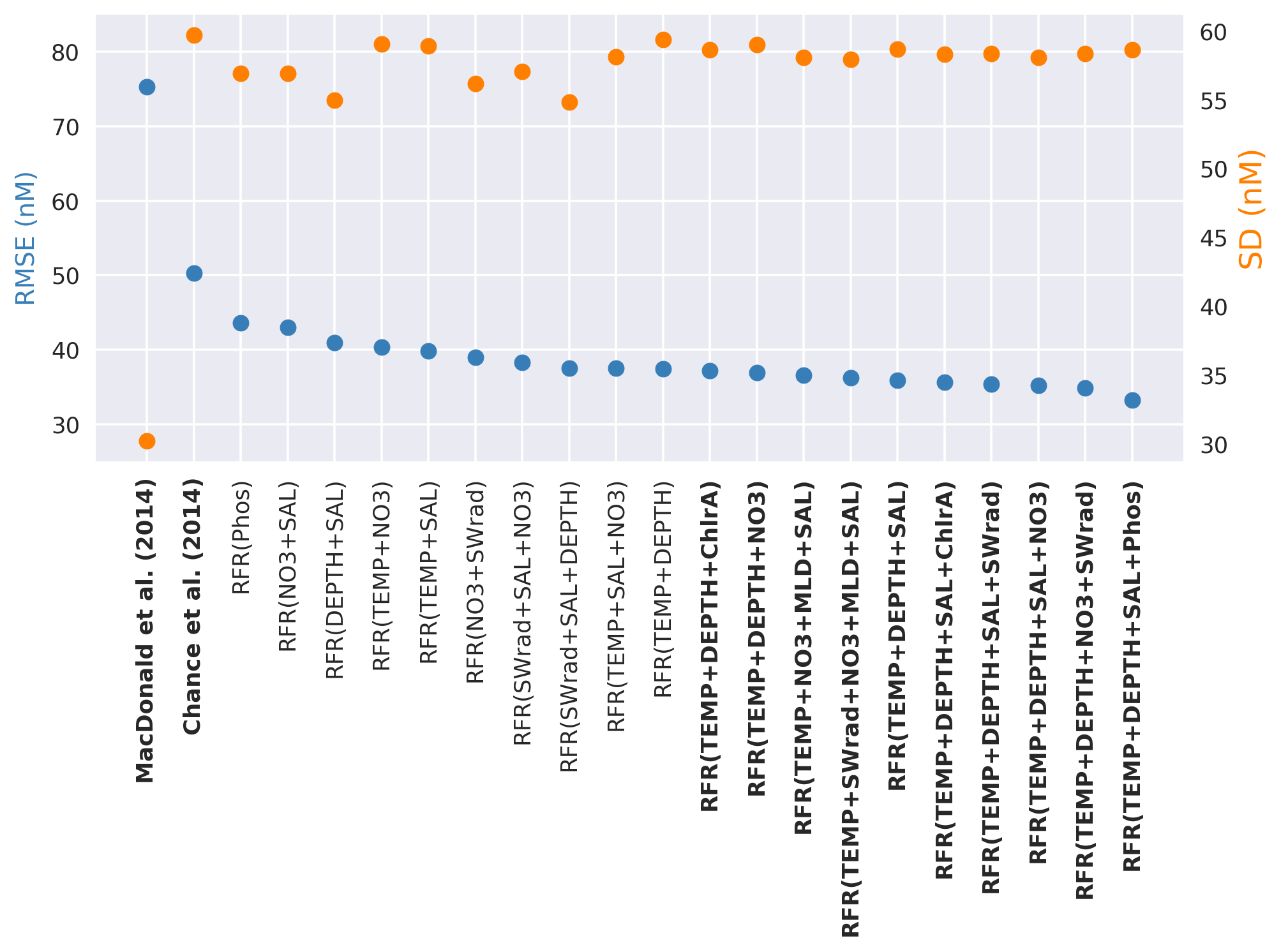
Figure 2Random forest regression (RFR) model performance (root mean square error (RMSE), blue) against the withheld data for the top 20 models on the left-hand y axis, along with values from the parameterisations from Chance et al. (2014) and MacDonald et al. (2014). The right-hand y axis is standard deviation of the prediction for the withheld data (orange). The top 10 performing models and the two exiting parameterisations considered here (Chance et al., 2014; MacDonald et al., 2014) are shown in bold. Parameterisations are ordered by their RMSE. Abbreviations are given in Table 1.
The RMSE values in Fig. 2 show the increased skill present in the new predictions compared to the existing parameterisations. The RMSE improves from the 75.3 and 50.2 nM found for the Chance et al. (2014) and MacDonald et al. (2014) parameterisations, respectively, to 33.2–37.4 nM for the top 10 models created here. Only modest gains are seen in RMSE between models with three variables or more.
The best-performing model in the list is only marginally better than the 10th best-performing one; therefore there is not an obvious “best” performing set of ancillary variables. Thus going forward we use an ensemble prediction approach based on the mean value from an ensemble of the 10 top-performing models.
3.5 Model descriptions
Unlike many machine learning approaches, the random forest regressor algorithm is interpretable. The decision trees can be visualised to explain the main features driving the splits. Figure 3 shows schematically the whole regression approach taken here. Panel (a) shows single trees, of which 500 are built with the same input variables and then combined into forest (b). Then this forest is combined with the nine other top-performing models (made from different combinations of ancillary variables) to make an ensemble (c). The 10 predictions of (c) are then arithmetically averaged into a single prediction, which thus includes the predictions of 5000 trees with 10 different combinations of input variables. In Fig. 3a, the colour of a limb or “branch” following a node is given by the variable driving that split within the training dataset. For Fig. 3b and c it shows the percent of times that a variable drives that node within the forest. The value of the ancillary variable that sets the split is shown inside the circle (a, b, c). The thickness of the branch scales to the throughput of training dataset samples contained within that split. The trees are shown to a depth of five nodes for aesthetic reasons and due to increased divergence of the trees within a forest the deeper you go. However the trees themselves are unlimited in the depth they can reach.

Figure 3Schematic illustration of how (a) multiple decision trees are combined into (b) a forest and then combined into (c) a further 10-member ensemble. (a) shows individual trees in a forest. (b) represent a forest of 500 trees as a single figurative tree. (c) shows the 10 forests of 500 trees combined into a single prediction. The branches in plots (a)–(c) are coloured by the percentage of the decisions at a given node that are driven by a given variable. That value within the circle gives the value of the main ancillary variable driving a split. The thickness of branches gives the throughput of the dataset through a given node for single trees (a) or the average for plots of forests (b, c). The 10 forests shown as thumbnails in panel (c) are also shown in larger form in Appendix Fig. A5. Variable names are coloured as per the following coloured text: temperature (blue, ∘C), depth (orange, metres), chlorophyll a (green, mg m−3), salinity (pink, PSU), nitrate (brown, µg m−3), mixed layer depth (MLD; purple, metres), phosphate (red, µg m−3), and shortwave radiation (grey, W m−2).
The first and larger splits in the data at decision nodes in the models can be simply read, which can provide understanding of the main variables driving the initial and largest splits in the prediction. For all models in the ensemble, the initial split is driven by temperature, with a split occurring at around 21.1 ∘C (with a standard deviation of 1.2 ∘C). The data are then split by two further nodes from this, a left- and right-hand split (e.g. Fig. 3b). If depth or temperature is present as a variable, then they drive the majority of the next splits. If depth is not present as a variable, then either nitrate or mixed layer depth (MLD) is the most common variable to dictate the split in the data at the next node in the tree. Thus a qualitative way of interpreting the initial splits of the dataset would be to say that the model is primarily differentiating between warmer and shallower locations.
Here we evaluate the performance of the ensemble prediction against the observational dataset (Sect. 4.1), and then we explore the predicted global monthly surface concentrations (Sect. 4.2).
4.1 Prediction of iodide at observational locations
Figure 4 shows a point-by-point comparison between parameterised and observed iodide for the entire dataset, the withheld dataset, and the withheld coastal dataset and withheld non-coastal dataset. Predictions are shown for the ensemble random forest regressor approach described here and for both the Chance et al. (2014) and MacDonald et al. (2014) parameterisations. The root mean square errors of observed and predicted values are given in Fig. 4 and in Table 3.

Figure 4Regression plots showing comparisons between predicted values and observations in the entire (blue, N=1293) and withheld data (orange, N=259), withheld data classed as coastal (green, N=157), and the withheld data classed as non-coastal (pink, N=102). Solid lines give the orthogonal distance regression line of best fit. The dashed grey line gives the 1:1 line. Root mean square error for each line is annotated by subplot in nanomolar (nM).
Table 3Statistics for observations and predictions by the ensemble prediction (RFR(ensemble)) and existing parameterisations against the entire dataset of observations. The root mean square error is shown against the entire and the withheld data.
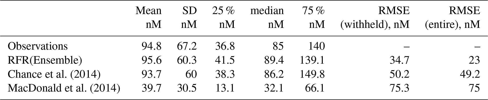
The new ensemble prediction is the best performing, with a lower RMSE (35 nM) compared to the existing parameterisations (75 and 50 nM for the MacDonald et al., 2014, and Chance et al., 2014, respectively) for the withheld data. Both the new parameterisation and Chance et al. (2014) parameterisation are relatively unbiased (both have best-fit-line slopes of 0.84, against the withheld data), but the new parameterisation shows less noise than Chance et al. (2014). MacDonald et al. (2014) shows a significant low bias and significant noise. The improved skill from the RFR ensemble is consistent for both coastal and non-coastal observations.
Figure 5 shows comparisons between the probability distribution functions (PDFs) of the observed iodide and the predictions, together with the PDFs of the biases for the entire, coastal, and non-coastal withheld datasets. The PDF of the new parameterisation shows the greatest similarity to the observations. The PDF from Chance et al. (2014) shows a similar range to the observations and structure to the observations, whereas the PDF from MacDonald et al. (2014) shows again a significant underestimate. The bias plots show the new predictions are generally clustered around zero with a relatively narrow peak. Chance et al. (2014) is again roughly clustered around zero but shows a wider peak. The largest biases are found from MacDonald et al. (2014), which systematically underestimates observed iodide concentrations.
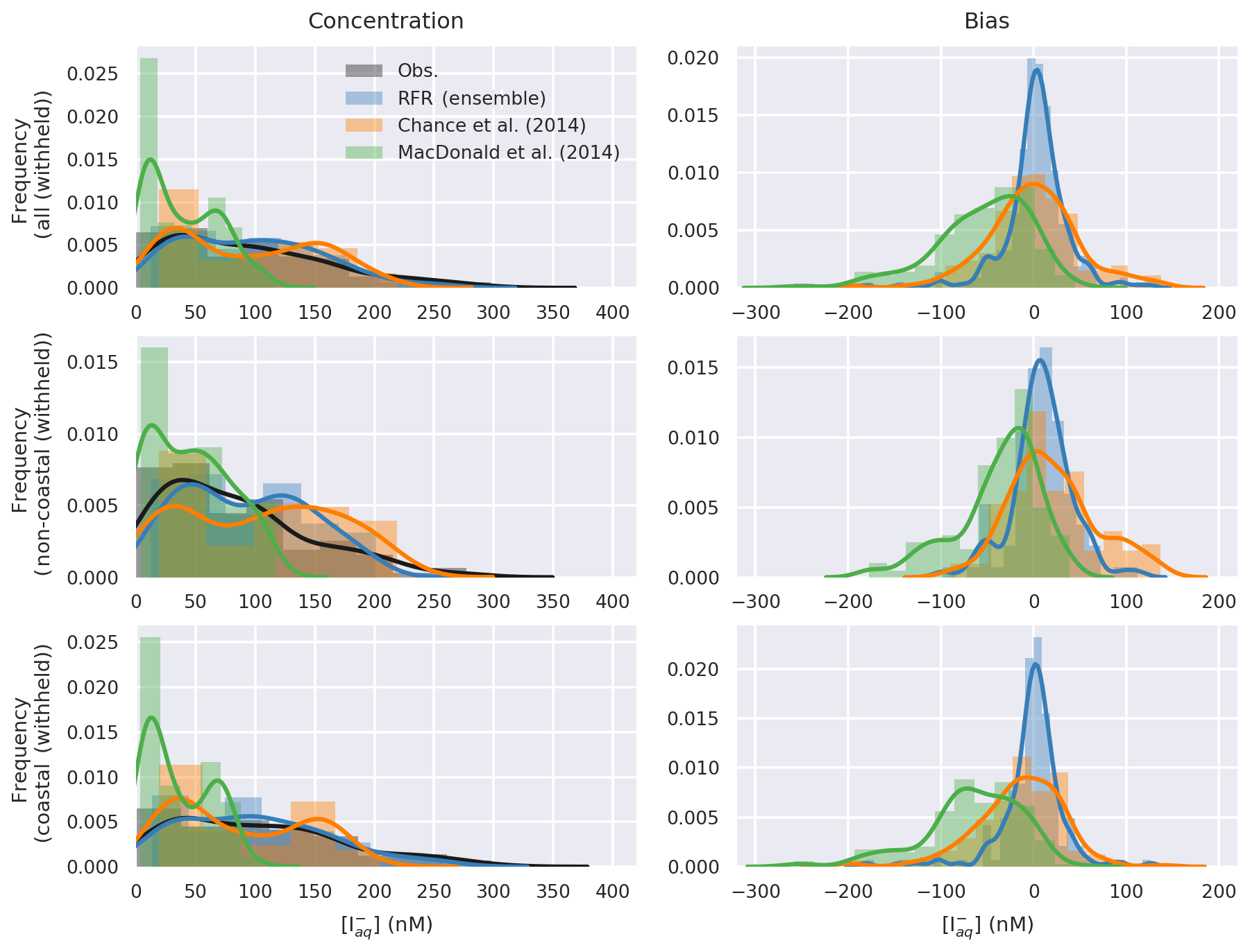
Figure 5Probability density function (bars) and Gaussian kernel density (lines) estimate of observations and predicted concentrations (left), and bias (right, model minus observations) in entire withheld dataset (upper, N=259), the withheld coastal dataset (middle, N=157), and the withheld non-coastal dataset (lower, N=102).
The dataset selection error range, which shows the influence of the choice of how the dataset is split into training and withheld data on model prediction, is described in Sect. 3.2. Within the 20-member ensemble of different testing/withdrawn choices, the average variation in RMSE was 8.4 nM (5.9–11.02 nM), and in the range of average predicted values it was 6.1 nM (5.4–6.6 nM). This translates to a percentage error range of 13.9 %–36.3 % on the RMSE and 5.4 %–7.3 % on the average predicted value.
The model selection error, which is the influence of the different independent variables used, is described in Sect. 3.2. The difference in the average prediction of the 10 members of the ensemble is 1.8 nM (with a range of average prediction from 96.0 to 97.8 nM), and the range of the difference in model performance is 3.9 nM (33.2–37.2 nM). As a percentage this model selection translates to a percentage uncertainty on the RMSE of 10.6 %–11.9 % and on the average of 1.8 %–1.9 %.
The dataset selection and model selection compare to an error on the observations of ∼10 %. Uncertainty from dataset selection has a far greater effect on the prediction error than model selection. This is expected due to the small dataset size. The combined error in the prediction (dataset selection + model selection error) is either comparable to (7.2 %–9.2 % in terms of average prediction) or greater (24 %–48 % in terms of RMSE) than the observational error.
From this analysis we have shown that the new ensemble RFR model performs significantly better than those currently in the literature. We now turn to explore the predicted global distribution of sea-surface iodide using our ensemble model.
4.2 Global sea-surface iodide distribution
From the ensemble prediction system we calculate monthly global grids (, ) of sea-surface iodide using the gridded ancillary data (Sect. 2). The annual average spatial predictions are shown in Fig. 6 with the observations overlaid in circles. Similar to previous work, annual average maximum concentrations of 220 nM are found in tropical and coastal regions (e.g. Oceania and in the Caribbean/Gulf of Mexico), with the lowest concentrations in mid-latitude waters (22.4 nM). Seasonal variability is also seen within the monthly prediction (Appendix Fig. A3). However, this spatial and temporal variability is not well constrained by observations. For example, some of the highest concentrations are predicted for the South China Sea, a region without any observations (Fig. 6). Some features visible in the concentration field appear to be associated with deep bathymetric features (e.g. the higher concentrations over the Mid-Atlantic Ridge – Fig. 6), even though a physical explanation for such a link seems unlikely.
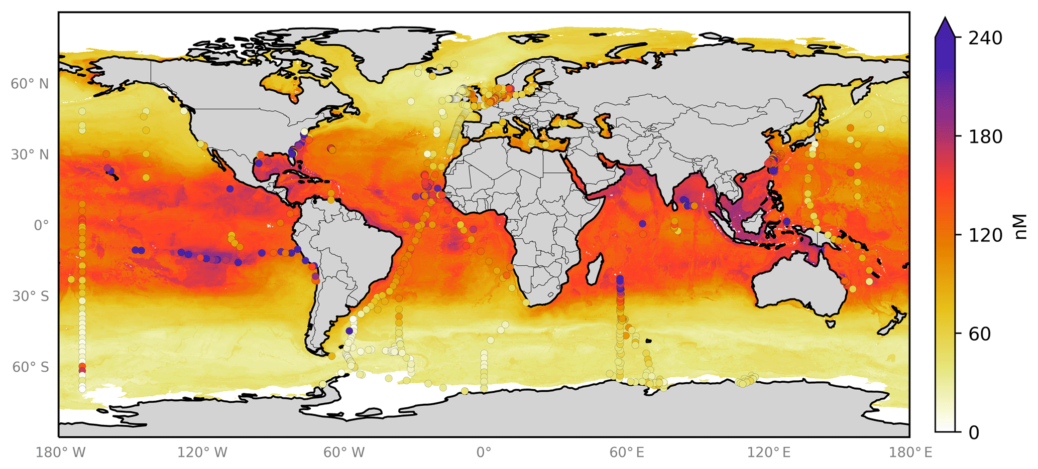
Figure 6Annual average predicted sea-surface iodide by the 10-member ensemble of models (RFR(Ensemble)), overlaid with iodide observations from Chance et al. (2019a) without outliers. Outliers are defined here as values greater than the third quartile plus 1.5 times the interquartile range (Frigge et al., 1989). Only locations that are entirely water are included in the spatial average. Earth raster and vector map data used are freely available from Natural Earth (http://www.naturalearthdata.com/, last access: 23 July 2019).
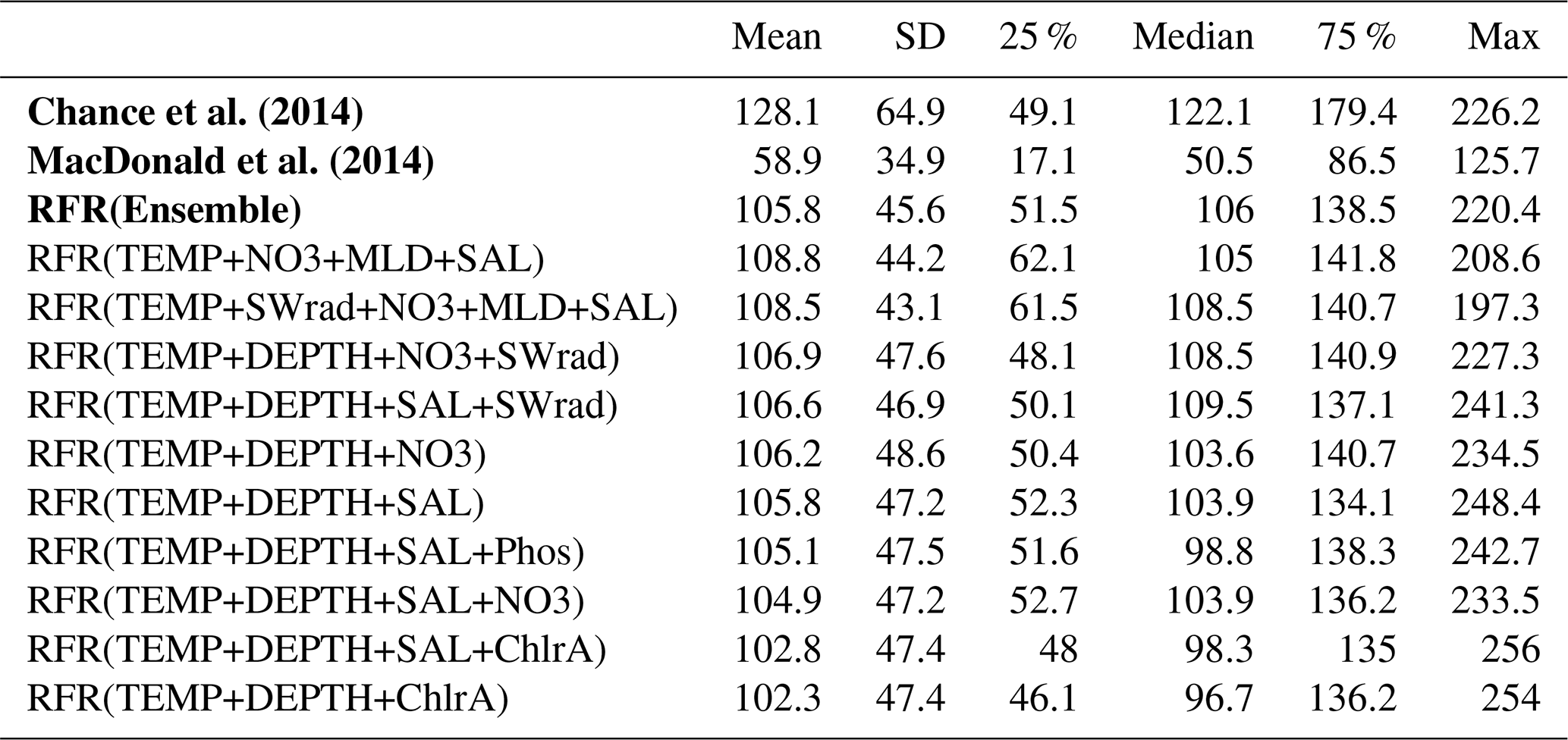
Summary statistics on the global predictions are shown in Table 4. These show that, as for comparisons at the observed locations (Sect. 4.1), the ensemble prediction is broadly in between the two existing parameters. The new ensemble model predicts a mean value of 106 nM (with members ranging from 102.3 to 108.8 nM), with predicted values from existing parameterisations ranging from 58.9 (MacDonald et al., 2014) to 128.1 nM (Chance et al., 2014).
Table 4Statistics on predicted global annual sea-surface values from new and existing parameters at a horizontal resolution of . Existing parameterisations (Chance et al., 2014; MacDonald et al., 2014) and the ensemble prediction are shown in bold.
The annual latitudinal average of these fields, together with predictions from Chance et al. (2014) and MacDonald et al. (2014), and the observations are shown in Fig. 7. Far greater structure is seen compared to the two existing parameterisations (Fig. 7) due to the multivariate and non-parametric ensemble approach used here. All parameterisations capture the broad observed feature of decreasing iodide from lower to higher latitude. The new predicted values lie between Chance et al. (2014) and MacDonald et al. (2014) in the tropics; however, within the polar regions, the new prediction is significantly higher than both of the previous parameterisations. The lower concentrations in the predicted values from MacDonald et al. (2014) for most of the global sea surface are clear.
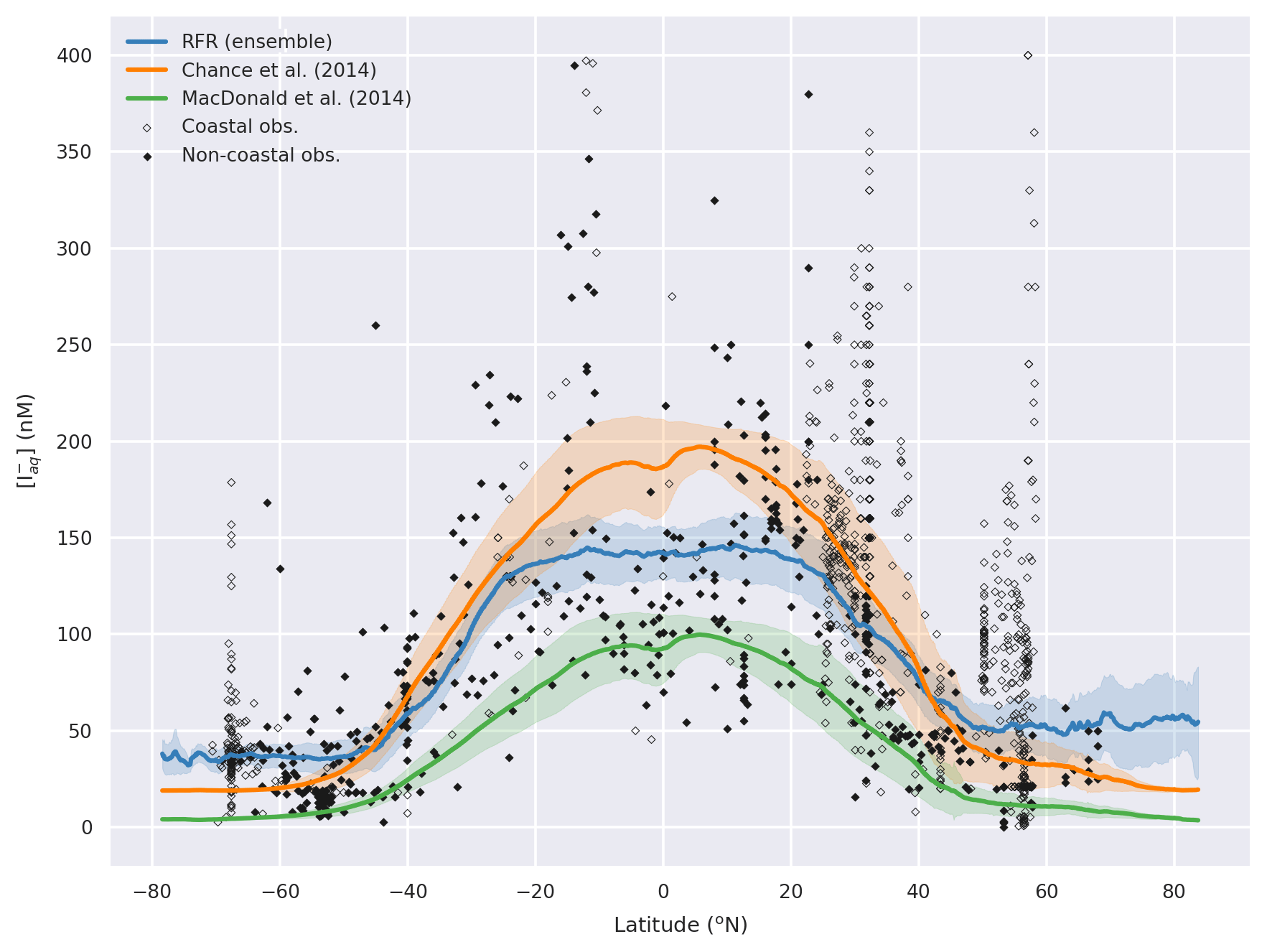
Figure 7Predicted annual average sea-surface iodide plotted against latitude (lines), overlaid with observed concentrations (diamonds). Solid lines give mean values and shaded regions give (±) the average standard deviation. The standard deviation is the monthly standard deviation across a latitude between all 10 ensemble members (RFR(Ensemble)) or within a single prediction for existing parameterisations (Chance et al., 2014; MacDonald et al., 2014). Filled diamonds show non-coastal observations and non-filled ones show coastal values. Extent of x axis is shown for grid boxes that are entirely water.
The range of dataset error is found for the 20 models with different training data splits, as described in Sect. 3.2. This gives an uncertainty in the form of a average range in predicted global mean surface iodide for all of the multiple builds of ensemble members of 4.0 nM (2.8–5.0) compared to a annual mean prediction of 106 nM. This maximum and minimum of this range in predicted values can then be divided by the minimum and maximum predicted global mean surface iodide values (98 and 109.3 nM, respectively) to give percent range of 2.5 % to 5.1 %. This is lower than that calculated for the individual locations of observations (Sect. 4.1) due to large global areas being similar in chemical and physical regimes compared to the subset of sampled locations within the observations.
The model selection error due to variability within ensembles' 10 members, generated with different independent variables, gives a global average surface concentration between 102.3 and 108.8 nM. This range in prediction gives a model selection error of 6.45 nM, which equates to 6.0 %–6.3 %. Like with the global uncertainty from dataset selection, the global value would be expected to be lower than the uncertainty at the specific locations of the observations (Sect. 4.1) due to the more homogeneous nature of the predicted areas. However, a greater variation is seen from different model predictions than within predictions for the observation locations. This highlights the importance of the different ancillary variables considered here and also therefore the strength gained from the ensemble approach taken here.
Within members of the ensemble, variation is modest except for two ensemble members which diverge north of N (Appendix Fig. A2). As noted earlier (Sect. 2), the values in this region are very poorly constrained by the observational dataset (Fig. 6).
In addition to the three errors described above, we also attempt to gain an understanding of the spatial uncertainty in the 10-model ensemble prediction. We do this by calculating the differences in the predicted spatial fields from the 10 ensemble members. Figure 8 shows the monthly average of the standard deviation of the 10 model ensemble as a percentage of the annual mean of the ensemble prediction. This is also shown in absolute terms in the Appendix (Fig. A4). Relative uncertainties are largest at the poles where predicted concentrations are lowest and where (at least in the Northern Hemisphere) very few observations are available to constrain the system. The southern oceans show an distinct pattern, where values close to coastal Antarctica appear well constrained but values further north appear poorly constrained.
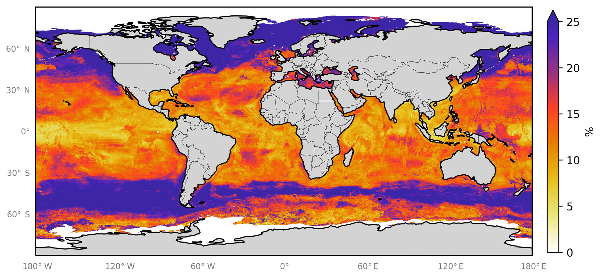
Figure 8Annual average spatial percent uncertainty in predicted sea-surface iodide for the ensemble of models. Percent spatial uncertainty was calculated as the standard deviation in monthly average values for all models, divided by the annual mean. Values are limited to 25 % for contrast, but the maximum plotted value is 77 % in the northern high latitudes. Only locations that are entirely water are included in the spatial average. Earth raster and vector map data used are freely available from Natural Earth (http://www.naturalearthdata.com/, last access: 23 July 2019).
The monthly ensemble mean and standard deviation between ensemble members for the main prediction presented here (RFR(Ensemble)), along with the individual ensemble members, are archived at the United Kingdom's Centre for Environmental Data Analysis (CEDA) as monthly files in NetCDF-4 format (Sherwen et al., 2019; https://doi.org/10/gfv5v3). To enable use in atmospheric and oceanic models, we have additionally bilinearly re-gridded the outputted fields onto common model grids (Appendix Table A4) using the open-source Python xESMF package (Zhuang, 2018). Values are provided for all locations globally and indices of land–water–ice cover are provided to allow data users to choose how to treat locations where water meets ice or land; however, we would not recommend the use of predicted values where ice or land are present. We recommended use of the standard output provided but have also provided the predictions made by the model with the Skagerrak dataset (Truesdale et al., 2003) included (which was excluded from the analysis presented here, as discussed further in Appendix Sect. A1).
Ancillary data extracted for observation locations and used to predict spatial fields are available from sources stated in Table 1. Iodide observations are described by Chance et al. (2019a) and made available by the British Oceanographic Data Centre (BODC, Chance et al., 2019b; https://doi.org/10/czhx).
Data analysis and processing used open-source Python packages, including Pandas (McKinney, 2010), Xarray (Hoyer and Hamman, 2017), and Scikit-learn (Pedregosa et al., 2011). Spatial re-gridding used the xESMF package (Zhuang, 2018). Plots presented here were created using the Matplotlib (Hunter, 2007), Seaborn (Waskom et al., 2017), and Cartopy (Elson et al., 2018) Python packages. The specific routines used for this work are archived within the sparse2spatial package (Sherwen, 2019), with the exception of the decision tree figures (Figs. 3 and A5), which were made using the TreeSurgeon package (Ellis and Sherwen, 2019).
Here we have explored the ability of an algorithmic approach combined with various physical and chemical variables to predict sea-surface iodide, without aiming to represent the biogeochemical or abiotic processes occurring. This approach instead gives a data-driven best guess at concentrations and an ability to quantify where the greatest uncertainty lies. However, certain features such as prediction of an apparent relationship between ocean bathymetry and sea-surface iodide concentrations, where the ocean is very deep (e.g. over the Mid-Atlantic Ridge), are unlikely to have a plausible physical explanation (Fig. 6).
The new spatial prediction presented here differs from what has been used previously in atmospheric models (e.g. Chance et al., 2014; MacDonald et al., 2014). Although the average value lies between these parameterisations, the prediction is closest to that from Chance et al. (2014) even with larger values found at higher latitudes. As most atmospheric models have used the iodide parameterisation from MacDonald et al. (2014) to calculate ocean iodine emissions (Appendix Table A1), a higher emission would therefore now be expected. This would result in larger decreases in tropospheric ozone burden than previously suggested (Sherwen et al., 2016a). A higher iodide sea-surface concentration would also result in a greater calculated ozone deposition (Ganzeveld et al., 2009; Luhar et al., 2017; Sarwar et al., 2016).
We have calculated the errors in sea-surface iodide concentrations at observational locations due to the dataset selection of 13.9 %–36.3 % and due to the model selection of 1.8 %–1.9 % (Sect. 4.1 and 4.2). These error estimates can be compared to an approximated error in the observations of ∼10 % (Chance et al., 2019a). Considering that the average predicted global concentration here is 106 nM (Sect. 4.2), these errors are notable. The greatest driver in error is the dataset selection. More observations, and particularly observations representative of under-sampled areas (e.g. Arctic) and seasons, will be required to reduce this error. The error caused by dataset selection is also reduced when the predictions are considered spatially over the global sea surface.
The choice of the algorithm used here is subjective and numerous other options are available. The random forest regressor was chosen due to its appropriateness for the continuous regression task performed here, its relatively cheap computation cost, and its interpretability. Considering the greatest uncertainty is driven by the paucity and sparsity of observations, using more complex techniques would not be expected to yield particularly different or drastically better results, considering other trade-offs.
We have developed a new way to build a spatially and temporally resolved dataset from a spatially and temporally sparse input of observations. This has allowed for the use of more observations than traditional approaches, which is particularly important with a paucity of data. This approach has demonstrated a large improvement in skill in terms of capturing observations compared to the existing parameterisations in use. It captures the pattern of decreasing iodide with higher latitude seen in the observations, as well as the greater spatial variation seen in the observations.
A1 Removed Skagerrak dataset
Ideally with sparse datasets as much data as possible would be included for training the regression models used. If a feature in the data is different enough to the rest of the dataset and not sufficiently represented for the regressor model to characterise it, then it has the potential to introduce a large dataset error (see Sect. 3.2 for details). This was shown when the iodide values above the outlier threshold were included (Sect. 3.2). There could be many other effects of including data that are significantly different to the rest of the dataset.
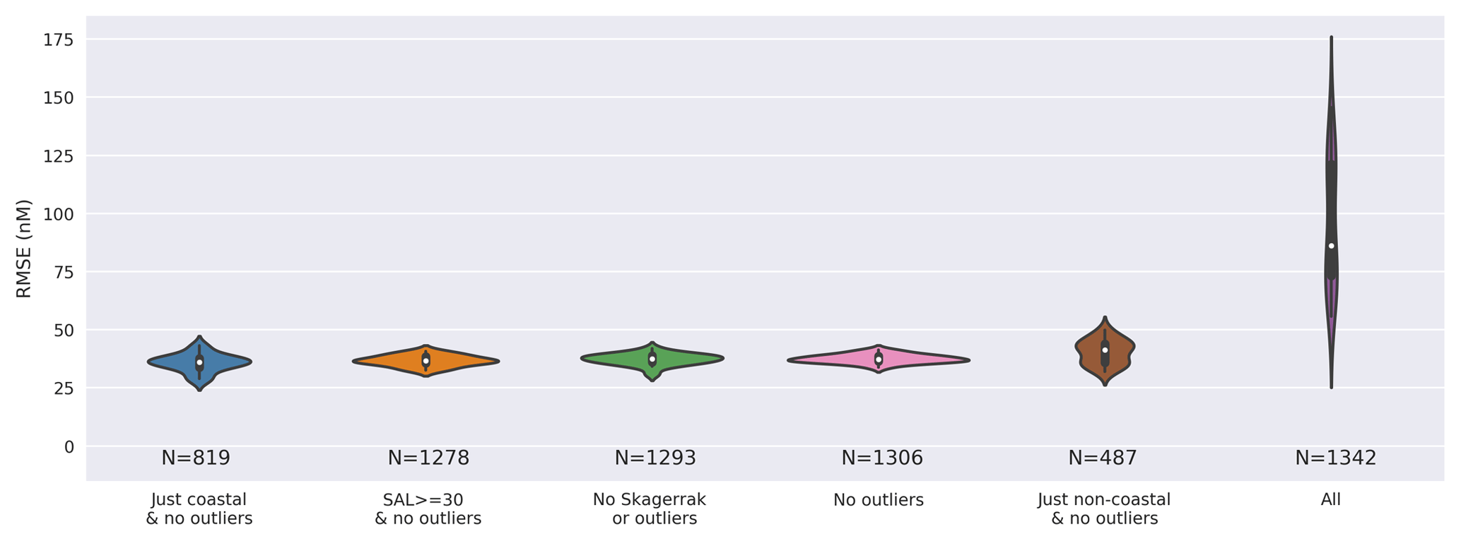
Figure A1Combined kernel density and violin plots showing the distribution of the root mean square error (RMSE) for 20 different models built from 20 different pseudo-random initialisations for a different selection of the dataset as described in Table 2 and Sect.3.2. Models built using the whole dataset (“all”), including outliers, show a significantly higher RMSE due to observations with higher iodide concentrations. The model used here includes ancillary variables of temperature, depth, and salinity which were thought to intuitively give a reasonable result.
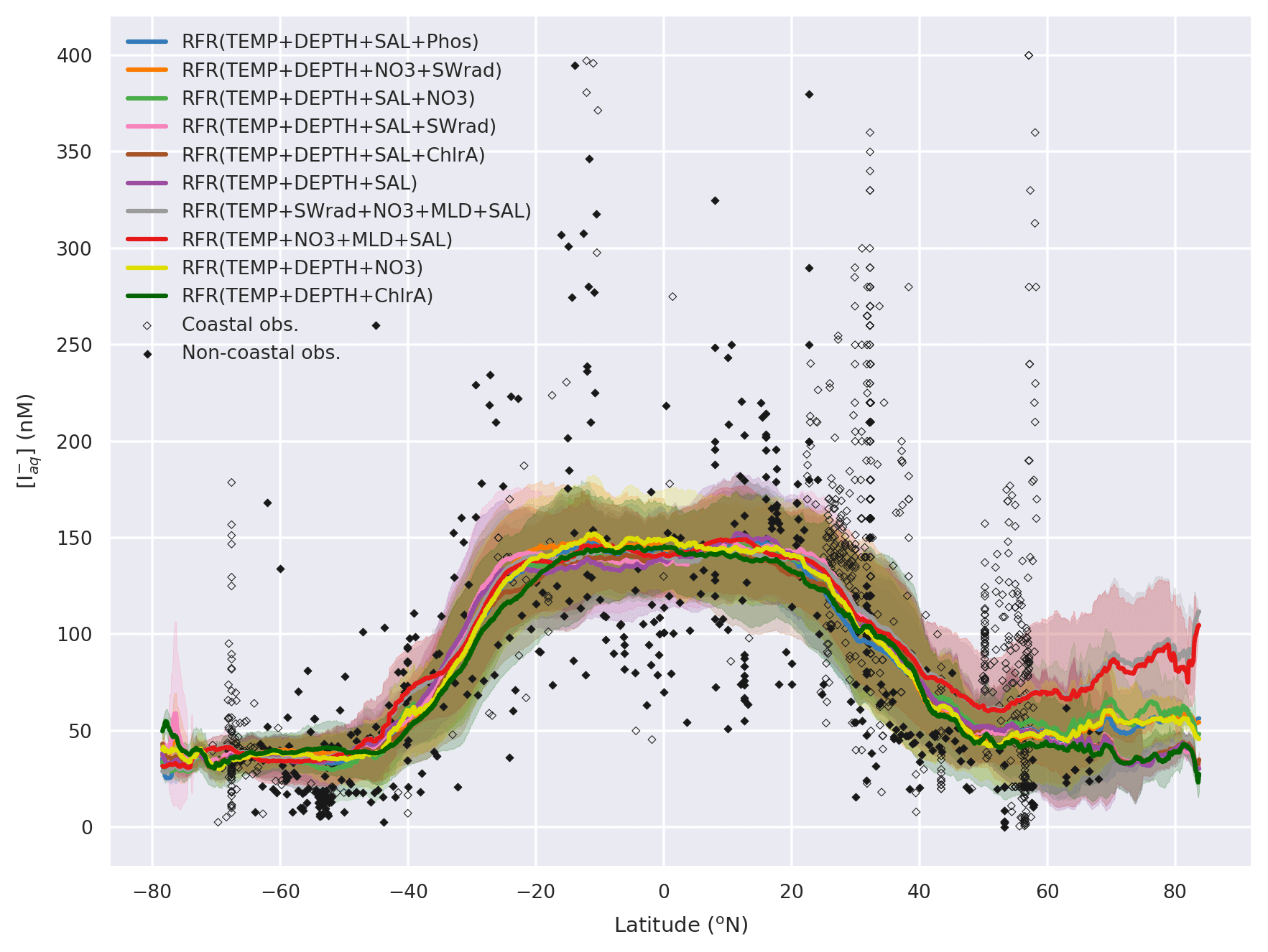
Figure A2Predicted global sea-surface iodide for all ensemble members plotted against latitude, overlaid with observed concentrations. Shaded regions give (±) the average standard deviation for a given latitude. The standard deviation is the monthly standard deviation for a single ensemble members (RFR(Ensemble)) or within a single prediction for existing parameterisations (Chance et al., 2014; MacDonald et al., 2014). Filled diamonds show non-coastal observations and unfilled ones show coastal values. Extent of x axis is shown for grid boxes that are entirely water.

Figure A3Percentage difference in monthly sea-surface iodide from the annual mean field predicted by the 10-model member ensemble. Only locations that are entirely water are included. Earth raster and vector map data used are freely available from Natural Earth (http://www.naturalearthdata.com/, last access: 23 July 2019).
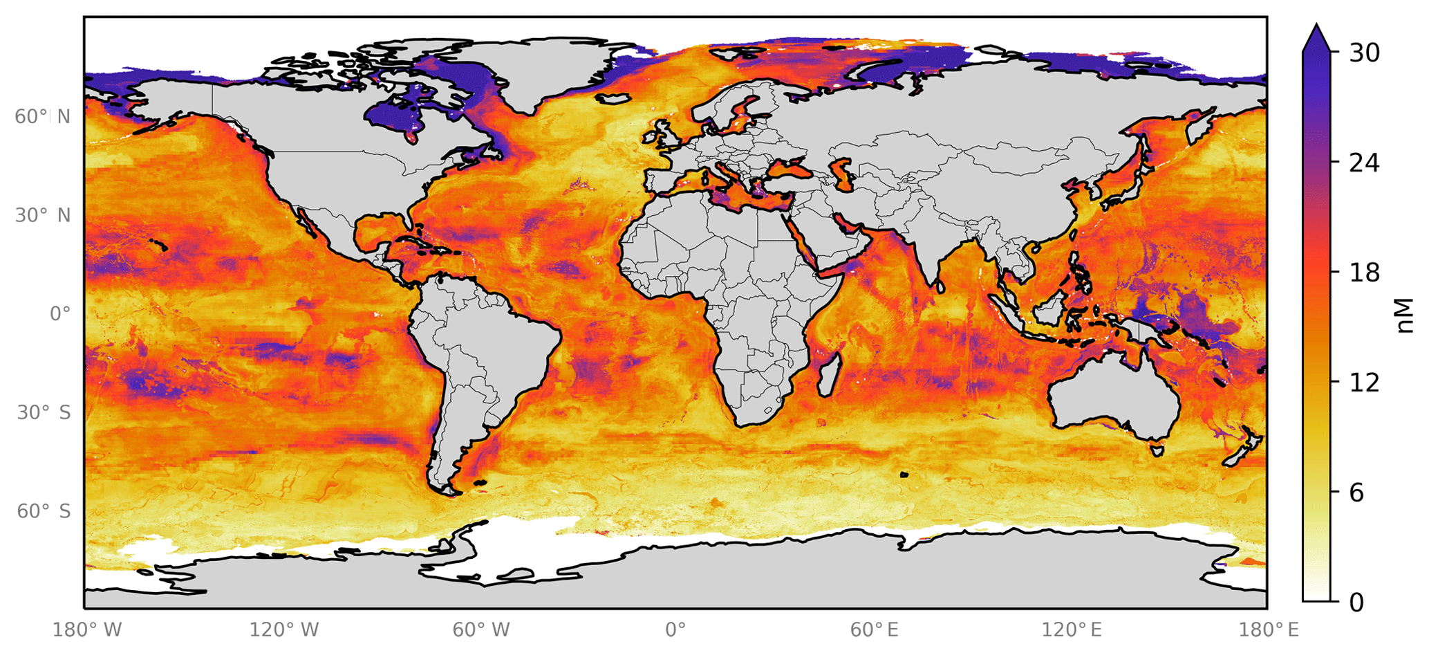
Figure A4Annual average spatial uncertainty in predicted sea-surface iodide for the ensemble of 10 models. Spatial variation was calculated as the standard deviation in monthly average values for all models. Values are limited to 30 nM for contrast, and the maximum value plotted is 52 nM in the northern high latitudes. Only locations that are entirely water are included in spatial the average. Earth raster and vector map data used are freely available from Natural Earth (http://www.naturalearthdata.com/, last access: 23 July 2019).

Figure A5Representation of all forests within the 10-member ensemble (also shown as thumbnails in Fig. 3c). The branches are coloured by percentage of each variable that drives the decision at a given node. The thickness of branches gives the average throughput of the dataset through a given node. Variable names are coloured as per the following coloured text: temperature (blue, ∘C), depth (orange,metres), chlorophyll a (green, mg m−3), salinity (pink, PSU), nitrate (brown, µg m−3), mixed layer depth (MLD; purple, metres), phosphate (red, µg m−3), and shortwave radiation (grey, W m−2)

Figure A6Predicted latitudinal average sea-surface iodide plotted against latitude, overlaid with observed concentrations. Figure is equivalent to Fig. 7, but the dashed line shows the prediction including data from the Skagerrak strait (Truesdale et al., 2003). Solid lines give mean values and shaded regions give ± the average standard deviation. For the ensemble the standard deviation is the monthly standard deviation within all ensemble members. Filled diamonds show non-coastal observations and unfilled ones show coastal values. Extent of x axis is shown for grid boxes that are entirely water.
The data from the Skagerrak strait (Truesdale et al., 2003), which are included in the (Chance et al., 2019a) compilation of iodide data, were excluded from this analysis. This is because, upon inclusion, high iodide at high latitudes ( N) is calculated (Appendix Fig. A6). An increasing trend is seen with latitude, reaching values comparable to the highest predicted values in the tropics. This region has a paucity of observations within the Chance et al. (2019a) compilation and there are none further north than Iceland. This means that any prediction in this region would be unconstrained by observations. Exclusion of these data leads to Fig. 7 where iodide is generally constant above 65∘ N.
The Skagerrak strait data (Truesdale et al., 2003) are also from a region where the observed ancillary variables compare poorly with those extracted from ancillary datasets. Observed salinity is between 24.0 and 33.5 PSU, whereas the climatological value is 31.7 to 35.8 PSU. This equates to a bias of the climatology versus the in situ observations of up to 9.6 PSU or 40 %. The Skagerrak is biogeochemically different from the Arctic, and its large influence on predicted values in the Arctic may arise simply from its latitudinal proximity, given the lack of observations from the regions themselves.
Chang et al. (2004)Oh et al. (2008)Coleman et al. (2010)Ganzeveld et al. (2009)Prados-Roman et al. (2015)Saiz-Lopez et al. (2014)Gantt et al. (2017)Sarwar et al. (2016, 2015)Sherwen et al. (2016a)Sherwen et al. (2016b, c, 2017a, b)Luhar et al. (2017, 2018)Table A1Summary of sea-surface iodide parameterisations in global and regional atmospheric models.
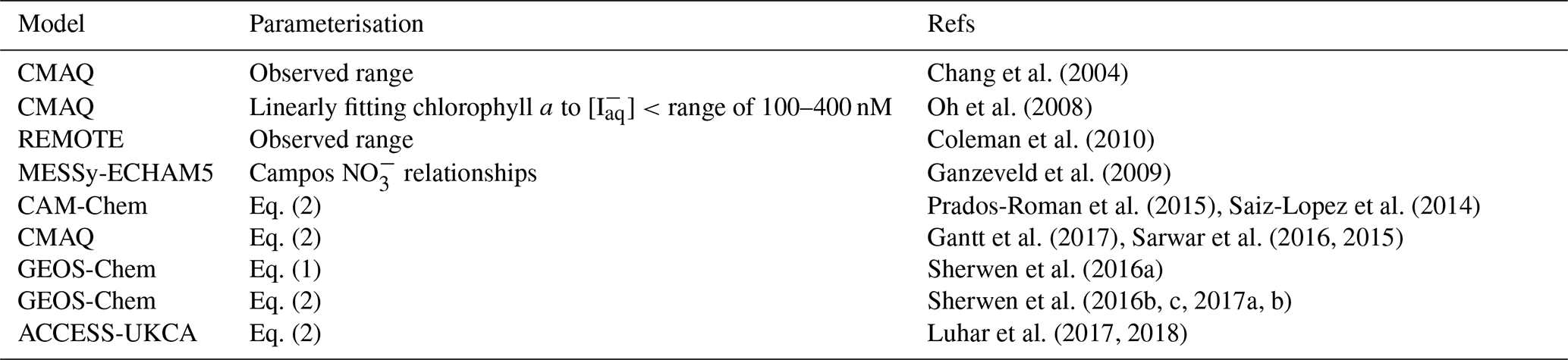
Table A2Statistics on observations and predicted values from the new ensemble and existing parameterisations at locations of observations. Root mean square error (RMSE) is shown against the withheld data and the entire dataset of observations. Ensemble members, ensemble prediction (RFR(Ensemble)), and existing parameterisations shown in bold. Values are shown for all 38 models built, including those not included in the ensemble.
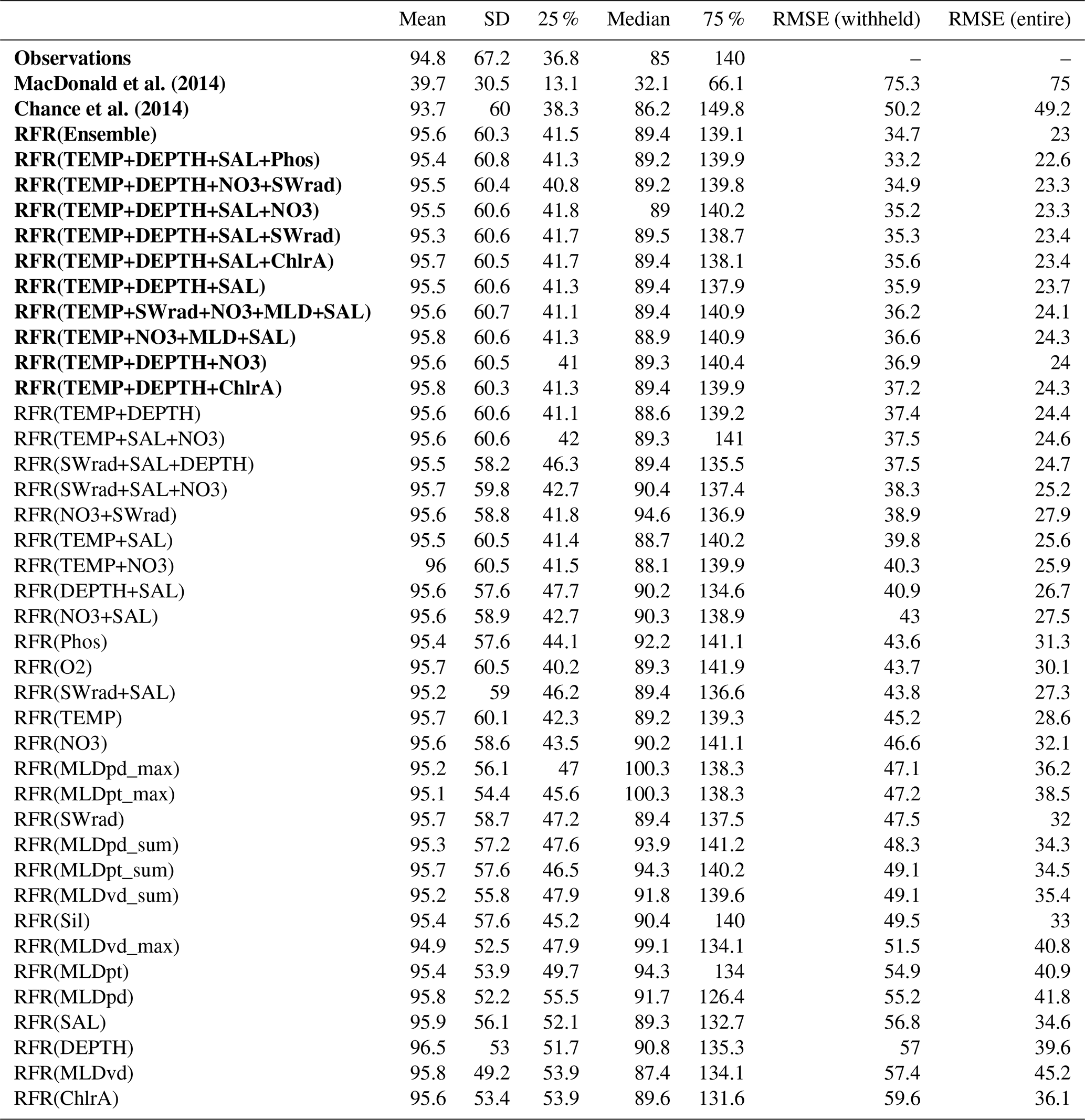
Table A3Statistics on observations and predicted values by ensemble and existing parameterisations at locations of observations but just for the withheld dataset locations. Table 3 shows the values for both the withheld and entire dataset.
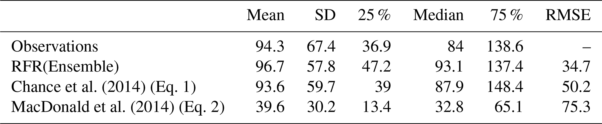
Table A4Spatial and temporal resolutions of global monthly iodide fields available for download from the United Kingdom's Centre from Environmental Data Analysis (Sherwen et al., 2019; https://doi.org/10/gfv5v3). Re-gridding was performed in Python using the open-source xESMF package (Zhuang, 2018).
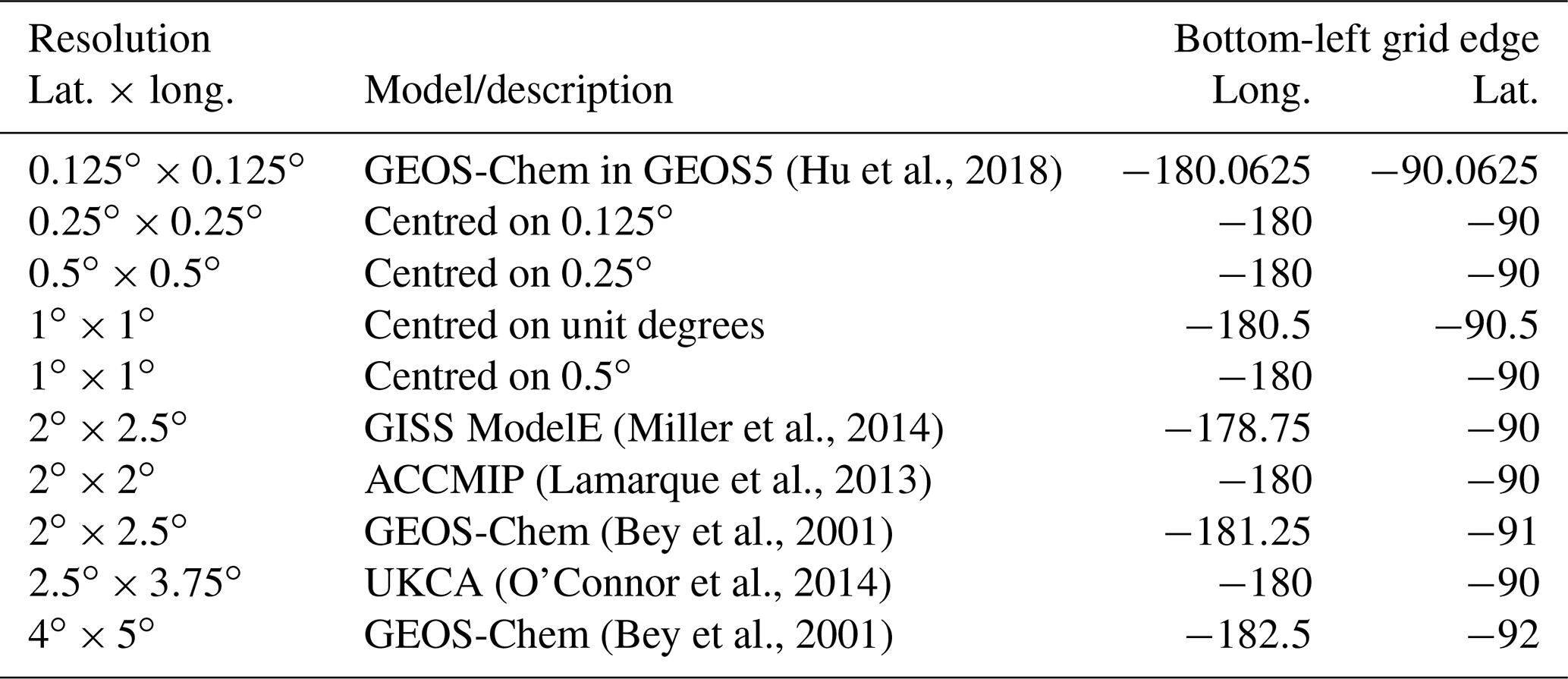
Latitudes less than indicate half-boxes at poles. Acronyms expand to United Kingdom Chemistry and Aerosols (UKCA), Atmospheric Chemistry and Climate Model Intercomparison Project (ACCMIP), and Goddard Institute for Space Studies (GISS).
The area this dataset is sampling in is also unusual in the Chance et al. (2019a) compilation due to its estuarine nature. However, this cannot entirely explain its behaviour as their are other estuarine datasets included (such as those from around the Chesapeake Bay, Luther and Cole, 1988; Wong and Cheng, 1998, 2008) which do not cause the same issue.
As the feature of high predicted Arctic iodide is driven by a single dataset of 19 samples (of which 4 would be removed as outliers) from a different region, it is highly uncertain. Not only do the in situ salinity observations compare poorly to the extracted ancillary ones, but the location itself represents a heterogeneity within the Chance et al. (2019b) compilation as it has relatively high observed iodide concentrations. It was therefore omitted from the analysis presented within this paper. However results with this dataset are included in the shared data outputs. It is hoped that further observations N can offer more insight into this uncertain region and also into the observations in the Skagerrak strait.
LJC, MJE, and TS conceived the work. TS developed the code, built the models, and performed the analysis. DE and TS wrote the code to make Fig. 3 and Appendix Fig. A5. TS wrote the paper with contributions from RJC, MJE, LT, and LJC.
The authors declare that they have no conflict of interest.
We all thank those who have provided their published and unpublished data to the Chance et al. (2019a) dataset and the British Oceanographic Data Centre (BODC) for hosting this, as well as all support staff involved.
We gratefully acknowledge those who have worked to compile and make available the ancillary datasets used here (Table 1). These include the World Ocean Atlas (WOA), Ocean Biology Processing Group (OBPG) at NASA's Goddard Space Flight Center, and the General Bathymetric Chart of the Oceans (GEBCO) teams.
We thank Tim Jickells, Peter Liss, David Stevens, and Martin Wadley for their useful conversations on and comments about this work.
We gratefully acknowledge funding from Natural Environment Research Council (NERC) through grants “Iodide in the ocean: distribution and impact on iodine flux and ozone loss” (NE/N009983/1) and “Big data for atmospheric chemistry and composition: Understanding the Science (BACCHUS)” (NE/L01291X/1).
This research has been supported by the Natural Environment Research Council grants “Iodide in the ocean: distribution and impact on iodine flux and ozone loss” (grant no. NE/N009983/1) and “Big data for atmospheric chemistry and composition: Understanding the Science (BACCHUS)” (grant no. NE/L01291X/1).
This paper was edited by Scott Stevens and reviewed by Peer Johannes Nowack and Laurens Ganzeveld.
Becker, J. J., Sandwell, D. T., Smith, W. H. F., Braud, J., Binder, B., Depner, J., Fabre, D., Factor, J., Ingalls, S., Kim, S.-H., Ladner, R., Marks, K., Nelson, S., Pharaoh, A., Trimmer, R., Rosenberg, J. V., Wallace, G., and Weatherall, P.: Global Bathymetry and Elevation Data at 30 Arc Seconds Resolution: SRTM30_PLUS, Mar. Geod., 32, 355–371, https://doi.org/10.1080/01490410903297766, 2009. a
Behrenfeld, M. J. and Falkowski, P. G.: Photosynthetic rates derived from satellite-based chlorophyll concentration, Limnol. Oceanogr., 42, 1–20, https://doi.org/10.4319/lo.1997.42.1.0001, 1997. a
Bey, I., Jacob, D. J., Yantosca, R. M., Logan, J. A., Field, B. D., Fiore, A. M., Li, Q., Liu, H. Y., Mickley, L. J., and Schultz, M. G.: Global modeling of tropospheric chemistry with assimilated meteorology: Model description and evaluation, J. Geophys. Res., 106, 23073–23095, https://doi.org/10.1029/2001JD000807, 2001. a, b
Breiman, L.: Random forests, Mach. Learn., 45, 5–32, 2001. a, b, c, d
Campos, M., Farrenkopf, A., Jickells, T., and Luther, G.: A comparison of dissolved iodine cycling at the Bermuda Atlantic Time-series Station and Hawaii Ocean Time-series Station, Deep Sea Res. Pt. II, 43, 455–466, https://doi.org/10.1016/0967-0645(95)00100-X, 1996. a
Carpenter, L. J., MacDonald, S. M., Shaw, M. D., Kumar, R., Saunders, R. W., Parthipan, R., Wilson, J., and Plane, J. M. C.: Atmospheric iodine levels influenced by sea surface emissions of inorganic iodine, Nat. Geosci., 6, 108–111, https://doi.org/10.1038/ngeo1687, 2013. a
Chameides, W. L. and Davis, D. D.: Iodine: Its possible role in tropospheric photochemistry, J Geophys. Res.-Oceans, 85, 7383–7398, https://doi.org/10.1029/JC085iC12p07383, 1980. a
Chance, R., Baker, A. R., Carpenter, L., and Jickells, T. D.: The distribution of iodide at the sea surface, Environ. Sci.-Proc. Imp., 16, 1841–1859, https://doi.org/10.1039/C4EM00139G, 2014. a, b, c, d, e, f, g, h, i, j, k, l, m, n, o, p, q, r, s, t, u, v, w, x, y, z, aa, ab, ac, ad
Chance, R., Tinel, L., Sherwen, T., Baker, A., Bell, T., Brindle, J., Campos, M., Croot, P., Ducklow, H., He, P., Hoogakker, B., Hopkins, F., Hughes, C., Jickells, T., Loades, D., Macaya, D., Mahajan, A., Malin, G., Phillips, D., Sinha, A., Sarkar, A., Roberts, I., Roy, R., Song, X., Winklebauer, H., Wuttig, K., Yang, M., Zhou, P., and Carpenter, L.: Global sea-surface iodide observations, 1967–2018, in review, 2019a. a, b, c, d, e, f, g, h, i, j, k, l
Chance, R., Tinel, L., Sherwen, T., Baker, A., Bell, T., Brindle, J., Campos, M., Croot, P., Ducklow, H., He, P., Hoogakker, B., Hopkins, F., Hughes, C., Jickells, T., Loades, D., Macaya, D., Mahajan, A., Malin, G., Phillips, D., Sinha, A., Sarkar, A., Roberts, I., Roy, R., Song, X., Winklebauer, H., Wuttig, K., Yang, M., Zhou, P., and Carpenter, L.: Global sea-surface iodide observations, 1967–2018, https://doi.org/10.5285/7e77d6b9-83fb-41e0-e053-6c86abc069d0, 2019b. a, b
Chance, R., Tinel, L., Sarkar, A., Sinha, A. K., Mahajan, A., Jickells, T. D., Stevens, D., Wadley, M., Chacko, R., Sabu, P., and Carpenter, L. J.: Surface inorganic iodine speciation in the Indian Ocean and Indian Ocean sector of the Southern Ocean, in preparation, 2019c. a
Chance, R. J., Shaw, M., Telgmann, L., Baxter, M., and Carpenter, L. J.: A comparison of spectrophotometric and denuder based approaches for the determination of gaseous molecular iodine, Atmos. Meas. Tech., 3, 177–185, https://doi.org/10.5194/amt-3-177-2010, 2010. a
Chang, W., Heikes, B. G., and Lee, M.: Ozone deposition to the sea surface: chemical enhancement and wind speed dependence, Atmos. Environ., 38, 1053–1059, https://doi.org/10.1016/j.atmosenv.2003.10.050, 2004. a, b
Coleman, L., Varghese, S., Tripathi, O. P., Jennings, S. G., and O'Dowd, C. D.: Regional-scale ozone deposition to North-East Atlantic waters, Adv. Meteorol., 2010, 243701, https://doi.org/10.1155/2010/243701, 2010. a, b
Cutter, G. A., Moffett, J. W., Nielsdóttir, M. C., and Sanial, V.: Multiple oxidation state trace elements in suboxic waters off Peru: In situ redox processes and advective/diffusive horizontal transport, Mar. Chem., 201, 77–89, https://doi.org/10.1016/J.MARCHEM.2018.01.003, 2018. a
Edwards, A. and Truesdale, V.: Regeneration of Inorganic Iodine Species in Loch Etive, a Natural Leaky Incubator, Estuar. Coast. Shelf S., 45, 357–366, https://doi.org/10.1006/ECSS.1996.0185, 1997. a
Ellis, D. and Sherwen, T.: wolfiex/TreeSurgeon: Wollemia, https://doi.org/10.5281/zenodo.3346817, 2019. a
Elson, P., Andrade, E. S. de, Hattersley, R., Campbell, E., Dawson, A., May, R., Little, B., Pelley, C., Blay, B., Donkers, K., Killick, P., Marqh, L., Peglar, P., Wilson, N., Kirkham, D., Bosley, C., Signell, J., Filipe, Krischer, L., Eriksson, D., Smith, A., Carlos, McDougall, D., Crosby, A., and Herzmann, D.: scaine1, Greg and munslowa: SciTools/cartopy: v0.17.0, https://doi.org/10.5281/ZENODO.1490296, 2018. a
Friedman, J. H., Hastie, T., and Tibshirani, R.: The elements of statistical learning: data mining, inference, and prediction, 2nd Edn., Springer, New York, NY, 2009. a, b
Frigge, M., Hoaglin, D. C., and Iglewicz, B.: Some implementations of the boxplot, Am. Stat., 43, 50–54, https://doi.org/10.1080/00031305.1989.10475612, 1989. a, b
Gantt, B., Sarwar, G., Xing, J., Simon, H., Schwede, D., Hutzell, W. T., Mathur, R., and Saiz-Lopez, A.: The impact of iodide-mediated ozone deposition and halogen chemistry on surface ozone concentrations across the continental United States, Environ. Sci. Technol., 51, 1458–1466, https://doi.org/10.1021/acs.est.6b03556, 2017. a, b
Ganzeveld, L., Helmig, D., Fairall, C. W., Hare, J., and Pozzer, A.: Atmosphere-ocean ozone exchange: A global modeling study of biogeochemical, atmospheric, and waterside turbulence dependencies, Global Biogeochem. Cy., 23, GB4021, https://doi.org/10.1029/2008GB003301, 2009. a, b, c, d, e
Garcia, H. E., Boyer, T. P., Locarnini, R. A., Antonov, J. I., Mishonov, A. V., Baranova, O. K., Zweng, M. M., Reagan, J. R., Johnson, D. R., and Levitus, S.: World Ocean Atlas 2013. Vol. 3: Dissolved Oxygen, Apparent Oxygen Utilization, and Oxygen Saturation, edited by: Levitus, S. and Mishonov, A., NOAA Atlas NESDIS 75, 27 pp., https://doi.org/10.7289/V5XG9P2W, 2010. a
Garcia, H. E., Locarnini, R. A., Boyer, T. P., Antonov, J. I., Baranova, O. K., Zweng, M. M., Reagan, J. R., Johnson, D. R., Mishonov, A. V., and Levitus, S.: World Ocean Atlas 2013. Vol. 4: Dissolved Inorganic Nutrients (phosphate, nitrate, silicate), edited by: Levitus, S. and Mishonov, A., NOAA Atlas NESDIS 76, 25 pp., 2014. a, b, c
Gardner, M. and Dorling, S.: Artificial neural networks (the multilayer perceptron) – a review of applications in the atmospheric sciences, Atmos. Environ., 32, 2627–2636, https://doi.org/10.1016/S1352-2310(97)00447-0, 1998. a
Hoyer, S. and Hamman, J.: xarray: N-D labeled arrays and datasets in Python, J. Open Res. Softw., 5, 10, https://doi.org/10.5334/jors.148, 2017. a
Hu, L., Keller, C. A., Long, M. S., Sherwen, T., Auer, B., Da Silva, A., Nielsen, J. E., Pawson, S., Thompson, M. A., Trayanov, A. L., Travis, K. R., Grange, S. K., Evans, M. J., and Jacob, D. J.: Global simulation of tropospheric chemistry at 12.5 km resolution: performance and evaluation of the GEOS-Chem chemical module (v10-1) within the NASA GEOS Earth system model (GEOS-5 ESM), Geosci. Model Dev., 11, 4603–4620, https://doi.org/10.5194/gmd-11-4603-2018, 2018. a, b
Hunter, J. D.: Matplotlib: A 2D graphics environment, Comput. Sci. Eng., 9, 90–95, https://doi.org/10.1109/MCSE.2007.55, 2007. a
Keller, C. A. and Evans, M. J.: Application of random forest regression to the calculation of gas-phase chemistry within the GEOS-Chem chemistry model v10, Geosci. Model Dev., 12, 1209–1225, https://doi.org/10.5194/gmd-12-1209-2019, 2019. a
Lamarque, J.-F., Shindell, D. T., Josse, B., Young, P. J., Cionni, I., Eyring, V., Bergmann, D., Cameron-Smith, P., Collins, W. J., Doherty, R., Dalsoren, S., Faluvegi, G., Folberth, G., Ghan, S. J., Horowitz, L. W., Lee, Y. H., MacKenzie, I. A., Nagashima, T., Naik, V., Plummer, D., Righi, M., Rumbold, S. T., Schulz, M., Skeie, R. B., Stevenson, D. S., Strode, S., Sudo, K., Szopa, S., Voulgarakis, A., and Zeng, G.: The Atmospheric Chemistry and Climate Model Intercomparison Project (ACCMIP): overview and description of models, simulations and climate diagnostics, Geosci. Model Dev., 6, 179–206, https://doi.org/10.5194/gmd-6-179-2013, 2013. a
Large, W. G. and Yeager, S. G.: The global climatology of an interannually varying air–sea flux data set, Clim. Dynam., 33, 341–364, https://doi.org/10.1007/s00382-008-0441-3, 2009. a
Lee, L. A., Carslaw, K. S., Pringle, K. J., Mann, G. W., and Spracklen, D. V.: Emulation of a complex global aerosol model to quantify sensitivity to uncertain parameters, Atmos. Chem. Phys., 11, 12253–12273, https://doi.org/10.5194/acp-11-12253-2011, 2011. a
Li, Q., Borge, R., Sarwar, G., de la Paz, D., Gantt, B., Domingo, J., Cuevas, C. A., and Saiz-Lopez, A.: Impact of halogen chemistry on air quality in coastal and continental Europe: application of CMAQ model and implication for regulation, Atmos. Chem. Phys. Discuss., https://doi.org/10.5194/acp-2019-171, in review, 2019. a
Locarnini, R. A., Mishonov, A. V., Antonov, J. I., Boyer, T. P., Garcia, H. E., Baranova, O. K., Zweng, M. M., Paver, C. R., Reagan, J. R., Johnson, D. R., Hamilton, M., and Seidov, D.: World Ocean Atlas 2013, Volume 1: Temperature, https://doi.org/10.1182/blood-2011-06-357442, 2013. a, b, c
Longhurst, A.: Ecological geography of the sea, Academic Press, San Diego, 1998. a
Lu, W., Ridgwell, A., Thomas, E., Hardisty, D. S., Luo, G., Algeo, T. J., Saltzman, M. R., Gill, B. C., Shen, Y., Ling, H.-F., Edwards, C. T., Whalen, M. T., Zhou, X., Gutchess, K. M., Jin, L., Rickaby, R. E. M., Jenkyns, H. C., Lyons, T. W., Lenton, T. M., Kump, L. R., and Lu, Z.: Late inception of a resiliently oxygenated upper ocean, Science, 361, 174–177, https://doi.org/10.1126/science.aar5372, 2018. a
Lu, Z., Hoogakker, B. A. A., Hillenbrand, C.-D., Zhou, X., Thomas, E., Gutchess, K. M., Lu, W., Jones, L., and Rickaby, R. E. M.: Oxygen depletion recorded in upper waters of the glacial Southern Ocean, Nat. Commun., 7, 11146, https://doi.org/10.1038/ncomms11146, 2016. a
Luhar, A. K., Galbally, I. E., Woodhouse, M. T., and Thatcher, M.: An improved parameterisation of ozone dry deposition to the ocean and its impact in a global climate–chemistry model, Atmos. Chem. Phys., 17, 3749–3767, https://doi.org/10.5194/acp-17-3749-2017, 2017. a, b, c
Luhar, A. K., Woodhouse, M. T., and Galbally, I. E.: A revised global ozone dry deposition estimate based on a new two-layer parameterisation for air–sea exchange and the multi-year MACC composition reanalysis, Atmos. Chem. Phys., 18, 4329–4348, https://doi.org/10.5194/acp-18-4329-2018, 2018. a, b
Luther, G. W. and Cole, H.: Iodine speciation in chesapeake bay waters, Mar. Chem., 24, 315–325, https://doi.org/10.1016/0304-4203(88)90039-4, 1988. a, b
MacDonald, S. M., Gómez Martín, J. C., Chance, R., Warriner, S., Saiz-Lopez, A., Carpenter, L. J., and Plane, J. M. C.: A laboratory characterisation of inorganic iodine emissions from the sea surface: dependence on oceanic variables and parameterisation for global modelling, Atmos. Chem. Phys., 14, 5841–5852, https://doi.org/10.5194/acp-14-5841-2014, 2014. a, b, c, d, e, f, g, h, i, j, k, l, m, n, o, p, q, r, s, t, u, v, w
McKinney, W.: Data Structures for Statistical Computing in Python, in: Proceedings of the 9th Python in Science Conference, edited by: van der Walt, S. and Millman, J., 51–56, 2010. a
Miller, R. L., Schmidt, G. A., Nazarenko, L. S., Tausnev, N., Bauer, S. E., Delgenio, A. D., Kelley, M., Lo, K. K., Ruedy, R., Shindell, D. T., Aleinov, I., Bauer, M., Bleck, R., Canuto, V., Chen, Y., Cheng, Y., Clune, T. L., Faluvegi, G., Hansen, J. E., Healy, R. J., Kiang, N. Y., Koch, D., Lacis, A. A., Legrande, A. N., Lerner, J., Menon, S., Oinas, V., Pérez García-Pando, C., Perlwitz, J. P., Puma, M. J., Rind, D., Romanou, A., Russell, G. L., Sato, M., Sun, S., Tsigaridis, K., Unger, N., Voulgarakis, A., Yao, M. S., and Zhang, J.: CMIP5 historical simulations (1850–2012) with GISS ModelE2, J. Adv. Model. Earth Syst., 6, 441–478, https://doi.org/10.1002/2013MS000266, 2014. a
Monterey, G. and Levitus, S.: Seasonal Variability of the Global Ocean Mixed Layer Depth, US Department of Commerce, National Oceanic and Atmospheric Administration, 1997. a
Nowack, P., Braesicke, P., Haigh, J., Abraham, N. L., Pyle, J., and Voulgarakis, A.: Using machine learning to build temperature-based ozone parameterizations for climate sensitivity simulations, Environ. Res. Lett, 13, 104016, https://doi.org/10.1088/1748-9326/aae2be, 2018. a
OBPG: NASA Goddard Space Flight Center, Ocean Biology Processing Group: Sea-viewing Wide Field-of-view Sensor (SeaWiFS) Ocean Color Data, NASA OB.DAAC, Greenbelt, MD, USA, Maintained by NASA Ocean Biology Distributed Active Archive Center (OB.DAAC), Goddard Spa, https://doi.org/10.5067/ORBVIEW-2/SEAWIFS_OC.2014.0, 2014. a
O'Connor, F. M., Johnson, C. E., Morgenstern, O., Abraham, N. L., Braesicke, P., Dalvi, M., Folberth, G. A., Sanderson, M. G., Telford, P. J., Voulgarakis, A., Young, P. J., Zeng, G., Collins, W. J., and Pyle, J. A.: Evaluation of the new UKCA climate-composition model – Part 2: The Troposphere, Geosci. Model Dev., 7, 41–91, https://doi.org/10.5194/gmd-7-41-2014, 2014. a
Oh, I.-B., Byun, D. W., Kim, H.-C., Kim, S., and Cameron, B.: Modeling the effect of iodide distribution on ozone deposition to seawater surface, Atmos. Environ., 42, 4453–4466, https://doi.org/10.1016/J.ATMOSENV.2008.02.022, 2008. a, b
Pedregosa, F., Varoquaux, G., Gramfort, A., Michel, V., Thirion, B., Grisel, O., Blondel, M., Prettenhofer, P., Weiss, R., Dubourg, V., and Others: Scikit-learn: Machine learning in Python, J. Mach. Learn. Res., 12, 2825–2830, 2011. a, b, c, d, e
Prados-Roman, C., Cuevas, C. A., Fernandez, R. P., Kinnison, D. E., Lamarque, J.-F., and Saiz-Lopez, A.: A negative feedback between anthropogenic ozone pollution and enhanced ocean emissions of iodine, Atmos. Chem. Phys., 15, 2215–2224, https://doi.org/10.5194/acp-15-2215-2015, 2015. a, b
Revell, L. E., Stenke, A., Tummon, F., Feinberg, A., Rozanov, E., Peter, T., Abraham, N. L., Akiyoshi, H., Archibald, A. T., Butchart, N., Deushi, M., Jöckel, P., Kinnison, D., Michou, M., Morgenstern, O., O'Connor, F. M., Oman, L. D., Pitari, G., Plummer, D. A., Schofield, R., Stone, K., Tilmes, S., Visioni, D., Yamashita, Y., and Zeng, G.: Tropospheric ozone in CCMI models and Gaussian process emulation to understand biases in the SOCOLv3 chemistry–climate model, Atmos. Chem. Phys., 18, 16155–16172, https://doi.org/10.5194/acp-18-16155-2018, 2018. a
Roshan, S. and DeVries, T.: Efficient dissolved organic carbon production and export in the oligotrophic ocean, Nat. Commun., 8, 2036, https://doi.org/10.1038/s41467-017-02227-3, 2017. a
Saiz-Lopez, A., Lamarque, J.-F., Kinnison, D. E., Tilmes, S., Ordóñez, C., Orlando, J. J., Conley, A. J., Plane, J. M. C., Mahajan, A. S., Sousa Santos, G., Atlas, E. L., Blake, D. R., Sander, S. P., Schauffler, S., Thompson, A. M., and Brasseur, G.: Estimating the climate significance of halogen-driven ozone loss in the tropical marine troposphere, Atmos. Chem. Phys., 12, 3939–3949, https://doi.org/10.5194/acp-12-3939-2012, 2012. a
Saiz-Lopez, A., Fernandez, R. P., Ordóñez, C., Kinnison, D. E., Gómez Martín, J. C., Lamarque, J.-F., and Tilmes, S.: Iodine chemistry in the troposphere and its effect on ozone, Atmos. Chem. Phys., 14, 13119–13143, https://doi.org/10.5194/acp-14-13119-2014, 2014. a, b
Saiz-Lopez, A., Baidar, S., Cuevas, C. A., Koenig, T. K., Fernandez, R. P., Dix, B., Kinnison, D. E., Lamarque, J.-F., Rodriguez-Lloveras, X., Campos, T. L., and Volkamer, R.: Injection of iodine to the stratosphere, Geophys. Res. Lett., 42, 6852–6859, https://doi.org/10.1002/2015GL064796, 2015. a
Sarwar, G., Gantt, B., Schwede, D., Foley, K., Mathur, R., and Saiz-Lopez, A.: Impact of Enhanced Ozone Deposition and Halogen Chemistry on Tropospheric Ozone over the Northern Hemisphere., Environ. Sci. Technol., 49, 9203–9211, https://doi.org/10.1021/acs.est.5b01657, 2015. a, b
Sarwar, G., Kang, D., Foley, K., Schwede, D., Gantt, B., and Mathur, R.: Technical note: Examining ozone deposition over seawater, Atmos. Environ., 141, 255–262, https://doi.org/10.1016/j.atmosenv.2016.06.072, 2016. a, b, c
Sherwen, T.: tsherwen/sparse2spatial: sparse2spatial v.0.1.1 – Predictions for iodide, CH2Br2 and CHBr3, https://doi.org/10.5281/zenodo.3349646, 2019. a
Sherwen, T., Evans, M. J., Carpenter, L. J., Andrews, S. J., Lidster, R. T., Dix, B., Koenig, T. K., Sinreich, R., Ortega, I., Volkamer, R., Saiz-Lopez, A., Prados-Roman, C., Mahajan, A. S., and Ordóñez, C.: Iodine's impact on tropospheric oxidants: a global model study in GEOS-Chem, Atmos. Chem. Phys., 16, 1161–1186, https://doi.org/10.5194/acp-16-1161-2016, 2016a. a, b, c, d
Sherwen, T., Evans, M. J., Spracklen, D. V., Carpenter, L. J., Chance, R., Baker, A. R., Schmidt, J. A., and Breider, T. J.: Global modelling of tropospheric iodine aerosol, Geophys. Res. Lett., 43, 10 012–10 019, https://doi.org/10.1002/2016GL070062, 2016b. a
Sherwen, T., Schmidt, J. A., Evans, M. J., Carpenter, L. J., Großmann, K., Eastham, S. D., Jacob, D. J., Dix, B., Koenig, T. K., Sinreich, R., Ortega, I., Volkamer, R., Saiz-Lopez, A., Prados-Roman, C., Mahajan, A. S., and Ordóñez, C.: Global impacts of tropospheric halogens (Cl, Br, I) on oxidants and composition in GEOS-Chem, Atmos. Chem. Phys., 16, 12239–12271, https://doi.org/10.5194/acp-16-12239-2016, 2016c. a
Sherwen, T., Evans, M. J., Carpenter, L. J., Schmidt, J. A., and Mickley, L. J.: Halogen chemistry reduces tropospheric O3 radiative forcing, Atmos. Chem. Phys., 17, 1557–1569, https://doi.org/10.5194/acp-17-1557-2017, 2017a. a, b, c
Sherwen, T., Evans, M. J. J., Sommariva, R., Hollis, L. D. J., Ball, S., Monks, P., Reed, C., Carpenter, L., Lee, J. D., Forster, G., Bandy, B., Reeves, C., and Bloss, W.: Effects of halogens on European air-quality, Faraday Discuss., 200, 75–100, https://doi.org/10.1039/C7FD00026J, 2017b. a, b, c, d
Sherwen, T., Chance, R., Tinel, L., Ellis, D., Evans, M., and Carpenter, L.: Global predicted sea-surface iodide concentrations v0.0.1, https://doi.org/10.5285/6448e7c92d4e48188533432f6b26fe22, 2019. a, b, c, d
Smith, W. H. F. and Sandwell, D. T.: Global Sea Floor Topography from Satellite Altimetry and Ship Depth Soundings, Science, 277, 1956–1962, https://doi.org/10.1126/science.277.5334.1956, 1997. a
Tong, W., Hong, H., Fang, H., Xie, Q., and Perkins, R.: Decision Forest: Combining the Predictions of Multiple Independent Decision Tree Models, J. Chem. Inf. Model., 43, 525–531, https://doi.org/10.1021/ci020058s, 2003. a
Truesdale, V. W., Danielssen, D. S., and Waite, T. J.: Summer and winter distributions of dissolved iodine in the Skagerrak, Estuar. Coast. Shelf S., 57, 701–713, https://doi.org/10.1016/S0272-7714(02)00412-2, 2003. a, b, c, d, e, f, g
Tsunogai, S. and Henmi, T.: Iodine in the surface water of the ocean, J. Oceanogr. Soc. Jpn., 27, 67–72, https://doi.org/10.1007/BF02109332, 1971. a, b
Waskom, M., Botvinnik, O., O'Kane, D., Hobson, P., Lukauskas, S., Gemperline, D. C., Augspurger, T., Halchenko, Y., Cole, J. B., Warmenhoven, J., de Ruiter, J., Pye, C., Hoyer, S., Vanderplas, J., Villalba, S., Kunter, G., Quintero, E., Bachant, P., Martin, M., Meyer, K., Miles, A., Ram, Y., Yarkoni, T., Williams, M. L., Evans, C., Fitzgerald, C., Fonnesbeck, C. B., Lee, A., and Qalieh, A.: mwaskom/seaborn: v0.8.1 (September 2017), https://doi.org/10.5281/ZENODO.883859, 2017. a
Wong, G. T. and Cheng, X. H.: Dissolved inorganic and organic iodine in the Chesapeake Bay and adjacent Atlantic waters: Speciation changes through an estuarine system, Mar. Chem., 111, 221–232, https://doi.org/10.1016/j.marchem.2008.05.006, 2008. a
Wong, G. T. F.: The marine geochemistry of iodine, Rev. Aquat. Sci., 4, 45–73, 1991. a
Wong, G. T. F. and Cheng, X. H.: Dissolved organic iodine in marine waters: Determination, occurrence and analytical implications, Mar. Chem., 59, 271–281, https://doi.org/10.1016/S0304-4203(97)00078-9, 1998. a, b, c
Zhou, X., Jenkyns, H. C., Owens, J. D., Junium, C. K., Zheng, X.-Y., Sageman, B. B., Hardisty, D. S., Lyons, T. W., Ridgwell, A., and Lu, Z.: Upper ocean oxygenation dynamics from I/Ca ratios during the Cenomanian-Turonian OAE 2, Paleoceanography, 30, 510–526, https://doi.org/10.1002/2014PA002741, 2015. a
Zhuang, J.: JiaweiZhuang/xESMF: v0.1.1, https://doi.org/10.5281/ZENODO.1134366, 2018. a, b, c
Žic, V., Carić, M., and Ciglenečki, I.: The impact of natural water column mixing on iodine and nutrient speciation in a eutrophic anchialine pond (Rogoznica Lake, Croatia), Estuar. Coast. Shelf S., 133, 260–272, https://doi.org/10.1016/j.ecss.2013.09.008, 2013. a
Zweng, M. M., Reagan, J. R., Antonov, J. I., Locarnini, R. A., Mishonov, A. V., Boyer, T. P., Garcia, H. E., Baranova, O. K., Johnson, D. R., Seidov, D., and Biddle, M. M.: World ocean atlas 2013, Volume 2, Salinity, 2013. a