the Creative Commons Attribution 4.0 License.
the Creative Commons Attribution 4.0 License.
 | 22 Aug 2019
Monthly gridded data product of northern wetland methane emissions based on upscaling eddy covariance observations
Timo Vesala
Olle Räty
Pavel Alekseychik
Mika Aurela
Bogdan Chojnicki
Ankur R. Desai
Albertus J. Dolman
Eugenie S. Euskirchen
Thomas Friborg
Mathias Göckede
Manuel Helbig
Elyn Humphreys
Robert B. Jackson
Georg Jocher
Fortunat Joos
Janina Klatt
Sara H. Knox
Natalia Kowalska
Lars Kutzbach
Sebastian Lienert
Annalea Lohila
Ivan Mammarella
Daniel F. Nadeau
Mats B. Nilsson
Walter C. Oechel
Matthias Peichl
Thomas Pypker
William Quinton
Janne Rinne
Torsten Sachs
Mateusz Samson
Hans Peter Schmid
Oliver Sonnentag
Christian Wille
Donatella Zona
Tuula Aalto
Natural wetlands constitute the largest and most uncertain source of methane (CH4) to the atmosphere and a large fraction of them are found in the northern latitudes. These emissions are typically estimated using process (“bottom-up”) or inversion (“top-down”) models. However, estimates from these two types of models are not independent of each other since the top-down estimates usually rely on the a priori estimation of these emissions obtained with process models. Hence, independent spatially explicit validation data are needed. Here we utilize a random forest (RF) machine-learning technique to upscale CH4 eddy covariance flux measurements from 25 sites to estimate CH4 wetland emissions from the northern latitudes (north of 45∘ N). Eddy covariance data from 2005 to 2016 are used for model development. The model is then used to predict emissions during 2013 and 2014. The predictive performance of the RF model is evaluated using a leave-one-site-out cross-validation scheme. The performance (Nash–Sutcliffe model efficiency =0.47) is comparable to previous studies upscaling net ecosystem exchange of carbon dioxide and studies comparing process model output against site-level CH4 emission data. The global distribution of wetlands is one major source of uncertainty for upscaling CH4. Thus, three wetland distribution maps are utilized in the upscaling. Depending on the wetland distribution map, the annual emissions for the northern wetlands yield 32 (22.3–41.2, 95 % confidence interval calculated from a RF model ensemble), 31 (21.4–39.9) or 38 (25.9–49.5) Tg(CH4) yr−1. To further evaluate the uncertainties of the upscaled CH4 flux data products we also compared them against output from two process models (LPX-Bern and WetCHARTs), and methodological issues related to CH4 flux upscaling are discussed. The monthly upscaled CH4 flux data products are available at https://doi.org/10.5281/zenodo.2560163 (Peltola et al., 2019).


Methane (CH4) is the second most important anthropogenic greenhouse gas (GHG) in terms of radiative forcing after carbon dioxide (CO2): 34 times (GWP100, including climate-carbon feedbacks) as strong as CO2 (Ciais et al., 2013). CH4 has contributed ∼20% to the cumulative GHG-related global warming (Etminan et al., 2016). Deriving constraints on CH4 sources and sinks is thus of utmost importance. The net atmospheric CH4 budget is well constrained by precise CH4 mole fraction measurements around the globe, yet the contribution of individual sources and sinks to this aggregated budget remains poorly understood. This is primarily due to lack of data to constrain the modelling results (Saunois et al., 2016). In order to make more accurate predictions of the atmospheric CH4 budget in a changing climate, the response of the various sources and sinks to different drivers needs to be better identified and quantified.
Natural wetlands are the largest and quantitatively most uncertain source of CH4 to the atmosphere (Saunois et al., 2016). An ensemble of land surface models estimated global CH4 emissions from wetlands for the period 2003–2012 to be 185 Tg(CH4) yr−1 (range 153–227 Tg(CH4) yr−1) and for the same period inversion models estimated it to be 167 Tg(CH4) yr−1 (range 127–202 Tg(CH4) yr−1) (Saunois et al., 2016). This discrepancy between bottom-up (process model) and top-down (inversion model) estimates, as well as the range of variability, exemplifies the large uncertainty of the current estimate for natural wetland CH4 emissions. Sources of this uncertainty can be roughly divided into two categories: (1) uncertainty related to the global areal extent of wetlands (e.g. Petrescu et al., 2010; Bloom et al., 2017a; Zhang et al., 2016) and (2) uncertainties related to the key CH4 emission drivers and responses to these drivers (e.g. Bloom et al., 2017a; Saunois et al., 2017). Evaluation of the emission estimates is thus urgently needed, and results from these efforts will lead to refined process models. Process model improvements will also directly affect the uncertainty of inversion results since they provide important a priori information to the inversion models (Bergamaschi et al., 2013).
Boreal and arctic wetlands comprise up to 50 % of the total global wetland area (e.g. Lehner and Döll, 2004) and the wetlands in these northern latitudes substantially contribute to total terrestrial wetland CH4 emissions (ca. 27 %, based on the sum of regional budgets for boreal North America, Europe and Russia in Saunois et al., 2016). In wetlands, CH4 is produced by methanogenic Archaea under anaerobic conditions, and hence the production takes place predominantly under water-saturated conditions (e.g. Whalen, 2005). The microbial activity and the resulting CH4 production is thus controlled by the quality and quantity of the available substrates, competing electron acceptors, and temperature (Le Mer and Roger, 2001). Once produced, the CH4 can be emitted to the atmosphere via three pathways: ebullition, molecular diffusion through soil matrix and water column, or plant transport. If plants capable of transporting CH4 are present, plant transport is generally the dominating emission pathway (Knoblauch et al., 2015; Kwon et al., 2017; Waddington et al., 1996; Whiting and Chanton, 1992). A large fraction of CH4 transported via molecular diffusion is oxidized into CO2 by methanotrophic bacteria in the aerobic layers of wetland soils and hence never reaches the atmosphere (Sundh et al., 1995), whereas CH4 transported via ebullition and plant transport can largely bypass oxidation (Le Mer and Roger, 2001; McEwing et al., 2015). Furthermore, processes related to permafrost (e.g. active layer, thermokarst) and snow cover dynamics (e.g. snow melt, insulation) have an impact on CH4 flux seasonality and variability (Friborg et al., 1997; Helbig et al., 2017; Mastepanov et al., 2008; Zona et al., 2016; Zhao et al., 2016). Hence, wetland CH4 emissions to the atmosphere largely depend on interplay between various controls, including water table position, temperature, vegetation composition, methane consumption, availability of substrates and competing electron acceptors.
During the past 2 decades, eddy covariance (EC) measurements of wetland CH4 emissions have become more common, due to rapid development in sensor technology (e.g. Detto et al., 2011; Peltola et al., 2013, 2014). The latest generation of low-power and low-maintenance instruments are rugged enough for long-term field deployment (Nemitz et al., 2018; McDermitt et al., 2010); thus, the number of sites where CH4 flux measurements have been made is increasing. Due to this progress, EC CH4 flux synthesis studies have been emerging (Petrescu et al., 2015; Knox et al., 2019). Similar progress was made with CO2 and energy flux measurements in the 1990s and now these measurements form the backbone of the global EC measurement network FLUXNET (https://fluxnet.fluxdata.org/, last access: 6 August 2019), whose data have provided invaluable insights into terrestrial carbon and water cycles. Some of the most important results have been obtained by upscaling FLUXNET observations using machine-learning algorithms to evaluate terrestrial carbon balance components and evapotranspiration (Beer et al., 2010; Bodesheim et al., 2018; Jung et al., 2010, 2011, 2017; Mahecha et al., 2010). These results are now widely used by the modelling community to evaluate process model performance (e.g. Wu et al., 2017) and to validate satellite-derived carbon cycle data products (e.g. Sun et al., 2017; Y. Zhang et al., 2017).
In this study, we synthesized EC CH4 flux data from 25 EC CH4 flux sites and developed an observation-based monthly gridded data product of northern wetland CH4 emissions. We focus on northern wetlands (north of 45∘ N) due to their significance in the global CH4 budget and relatively good data coverage and process understanding, at least compared to tropical systems (Knox et al., 2019). High-latitude regions are projected to warm during the next century at a faster rate than any other region, which will likely significantly impact the carbon cycling of wetland ecosystems (Tarnocai, 2009; Z. Zhang et al., 2017) and permafrost areas of the Arctic boreal region (Schuur et al., 2015). To date, CH4 emission estimates for northern wetlands are typically based on process models (Bohn et al., 2015; Bloom et al., 2017a; Chen et al., 2015; Melton et al., 2013; Stocker et al., 2013; Wania et al., 2010; Watts et al., 2014; Zhang et al., 2016) or inversion modelling (Bohn et al., 2015; Bruhwiler et al., 2014; Spahni et al., 2011; Thompson et al., 2017; Thonat et al., 2017; Warwick et al., 2016), yet scaling of existing chamber measurements to the northern wetland area has also been published (Zhu et al., 2013). However, CH4 emission estimates obtained with the former two approaches are not independent since the attribution of CH4 emissions derived using inversion models to different emission sources (e.g. wetlands) depends largely on a priori estimates of these emissions (i.e. process models for wetland emissions), highlighting the tight coupling between these two approaches (Bergamaschi et al., 2013; Spahni et al., 2011). Hence, the main objective of this study is to produce an independent data-driven estimate of northern wetland CH4 emissions. This product could be used as an additional constraint for the wetland emissions and hence aid in process model refinement and development. Additionally, the drivers causing CH4 flux variability at the ecosystem scale are also evaluated and methodological issues are discussed, which will support future CH4 wetland flux upscaling studies.
Data from flux measurement sites (Fig. 1) were acquired and used together with forcing data to estimate CH4 emissions from northern wetlands with a monthly time resolution using a random forest (RF) modelling approach. Both in situ measurements and remote sensing are utilized in this study. In this section, the RF approach is briefly introduced (Sect. 2.1) and data selection, quality filtering, gap filling and aggregation to monthly values are described (Sect. 2.3). We identified 40.7 site years available for analysis, measured between 2005 and 2016. To perform upscaling to all wetlands north of 45∘ N, gridded data products of the flux drivers and wetland distribution maps were needed. These products are presented in Sect. 2.4 and 2.5, respectively. Finally, the upscaled wetland CH4 emissions are compared against process model outputs, with the models briefly described in Sect. 2.6.
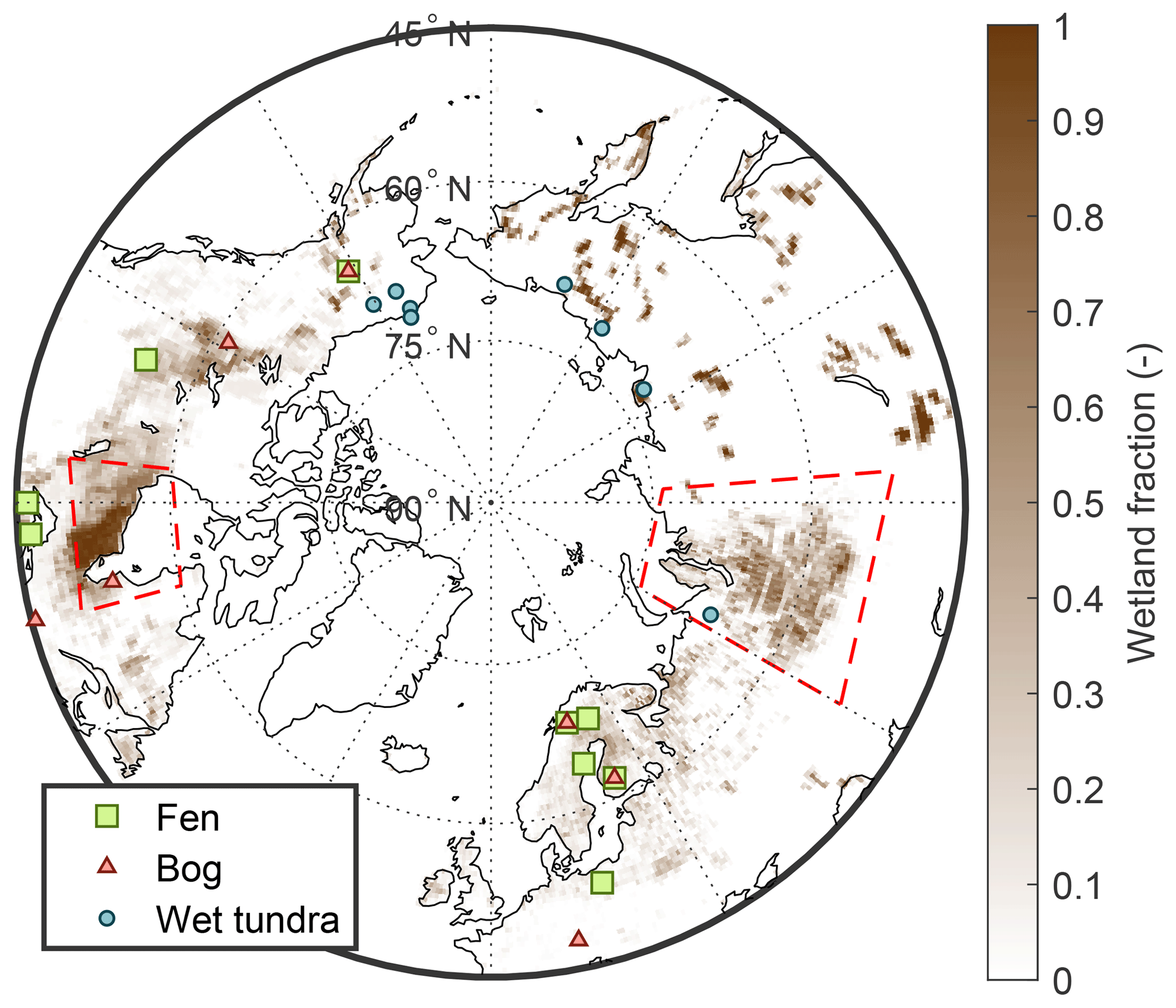
Figure 1Map showing the locations of the EC measurements. The distribution of wetlands shown in the figure is based on Xu et al. (2018). Hudson Bay lowlands (50–60∘ N, 75–96∘ W) and western Siberian lowlands (52–74∘ N, 60–94.5∘ E) are highlighted with dashed red lines.
Here, wetlands are defined as terrestrial ecosystems with water table positions near the land surface and with plants that have adapted to these waterlogged conditions. We exclude lakes, reservoirs and rivers from the study, in addition to ecosystems with significant human influence (e.g. drainage, rewetting). We consider peat-forming wetlands (i.e. mires), which can be further classified as fens and bogs based on hydrology, as well as wetlands with hydric mineral soils. Tundra wetlands may have only a shallow peat layer or none at all. Unified classifications for wetlands are still lacking, and typically different countries follow their own classification scheme, albeit some joint classification schema have been developed (e.g. Ramsar Classification System for Wetland Type).
2.1 Random forest algorithm
Random forest (RF) is a machine-learning algorithm that can be used for classification or regression analyses (Breiman, 2001). In this study the RF models consist of a large ensemble of regression trees. Each individual regression tree is built by training it with a random subset of training data and the trees are trained independently of each other. The RF model output is then the average of all the predictions made by individual regression trees in the forest. Hence, the RF algorithm applies the bootstrap aggregation (bagging) algorithm and takes full advantage of the fact that ensemble averaging decreases the noise of the prediction. In addition to random selection of training data, the predictor variables used in split nodes are also selected from a random sample of all predictors, which minimizes the possible correlation between trees in the forest (Breiman, 2001) and decreases the possibility of overfitting. The predictor variables can be either categorical or continuous. The variables are then used in the split nodes to divide the data into two (e.g. categorical variable true or false or a continuous variable, such as temperature above or below 5 ∘C).
Performance of RF algorithms to predict CO2 and energy fluxes across FLUXNET sites have been compared against other machine-learning algorithms, such as artificial neural networks and multivariate regression splines, by Tramontana et al. (2016), who showed that differences between methods were negligible. We anticipate a similarly negligible effect of machine-learning algorithm choice for CH4 fluxes. For a thorough description of the RF algorithm for flux upscaling purposes, the reader is referred to Bodesheim et al. (2018) (and references therein).
In this study, the RF models were developed using the MATLAB 9.4.0 (R2018a) TreeBagger function with default values similar to those of Bodesheim et al. (2018). These settings included a minimum of five samples in a leaf node and used mean squared error (MSE) as a metric for deciding the split criterion in split nodes. Each trained forest consisted of 300 randomized regression trees.
2.1.1 RF model development for CH4 flux gap filling
Our RF algorithm was used for gap filling the daily CH4 flux time series. The performance of the RF model was evaluated against “out-of-bag” (OOB) data (approximately one-third of data for each tree). Since each individual tree in the RF model was trained using a subset of training data, the rest of the data (i.e. OOB data) can be used as independent validation data to evaluate the prediction performance of that particular regression tree and hence the whole forest (Breiman, 2001). Only the five most important predictors were retained for the gap-filling models for each site. The relative importance of predictors (e.g. air temperature) was evaluated by randomly shuffling the predictor data and then estimating the increase in MSE when model output is compared against OOB data (Breiman, 2001). For important predictors, MSE will increase significantly due to shuffling, whereas the effect of shuffling on MSE is minor for less important predictors. Note that this procedure was executed separately for each site, and thus different predictors may have been used for different sites for gap filling.
2.1.2 RF model development for CH4 flux upscaling
For upscaling purposes, one RF model was developed using all the available data in order to maximize the information content for the global (>45∘ N) CH4 flux map. The model performance or uncertainty, however, was evaluated using two approaches. (1) The predictive performance of the model was assessed using the widely used “leave-one-site-out” cross-validation scheme (e.g. Jung et al., 2011). In order to avoid correlation between training data and validation data, sites located nearby (closer than 100 km) were excluded from the training data (Roberts et al., 2016). (2) The uncertainty of the upscaled fluxes was estimated by bootstrapping. The 200 independent RF models were trained using a bootstrap sample of the available data. This yielded 200 predictions for each grid cell and time step in the upscaled CH4 flux map. The variability over this prediction ensemble was used as an uncertainty measure following, e.g. Aalto et al. (2018) and Zhu et al. (2013). This uncertainty estimate reflects the ability of the RF model to capture the dependence of CH4 flux on the used predictors in the available data. However, it does not have any reference to actual in situ CH4 fluxes, unlike the model predictive performance estimated with cross-validation.
Predictors for the RF model used in the upscaling were determined following Moffat et al. (2010). First, the RF models were trained for each site using one predictor at a time (see all the predictors in Table 1). The single predictor which yielded the best match against validation data (leave-one-site-out scheme) was selected as the primary driver. Then, the RF models were trained again with the primary driver, plus each of the other predictors in turn as secondary drivers. Then the RF model performance was again evaluated and the best predictor pair was selected for the next round. This procedure was continued until all the predictors were included in the RF model. The smallest set of predictors capable of producing optimal RF model performance was used for flux upscaling.
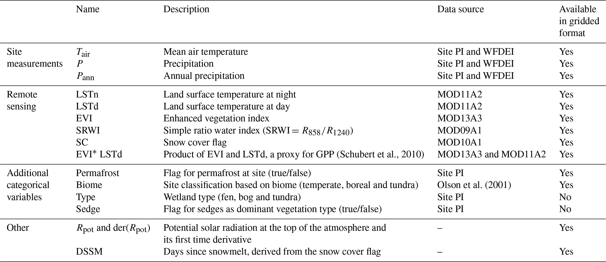
Table 1Description of input variables for RF model development for upscaling. Data were aggregated to monthly values (see text) unless otherwise noted below.
2.2 Metrics for model performance evaluation
The RF model performance was evaluated against independent validation data using a set of statistical metrics, which were related to different aspects of model performance. During the RF model training MSE was optimized as follows:
where o and p are vectors containing the observed and predicted values, respectively, and the overbar denotes averaging.
The Nash–Sutcliffe model efficiency (NSE; Nash and Sutcliffe, 1970) was used to evaluate how well the model was able to predict validation data when compared against a reference (typically the mean of the validation data):
where i is index running over all the n values in the o and p vectors. When NSE is equal to 1, there is a perfect match between prediction and observations. Values above 0 imply that the model predicts the observations better than the mean of observations and values below 0 indicate that the predictive capacity of the model is worse than the mean of validation data. Note that NSE calculated with Eq. (2) above is equivalent to the coefficient of determination calculated using residual sum of squares and total sum of squares. However, following the approach used in previous upscaling studies (e.g. Bodesheim et al., 2018; Tramontana et al., 2016), we opted to call this metric NSE. Instead, the coefficient of determination (R2) was estimated as the squared Pearson correlation coefficient. Note that R2 and NSE are equal when there is no bias between o and p and the residuals follow Gaussian distribution. Pearson correlation coefficients obtained with different model runs are compared using Fisher's r to z transformation.
The standard deviation (σ) of the model residuals was used to evaluate the spread of model residual values (RE):
whereas biases between model predictions and validation data were used to estimate the systematic uncertainty in the upscaled fluxes (BE):
Note that RE equals RMSE when there is no systematic difference between the model predictions and observations (i.e. when BE equals zero).
2.3 Data
2.3.1 Data from eddy covariance flux measurement sites
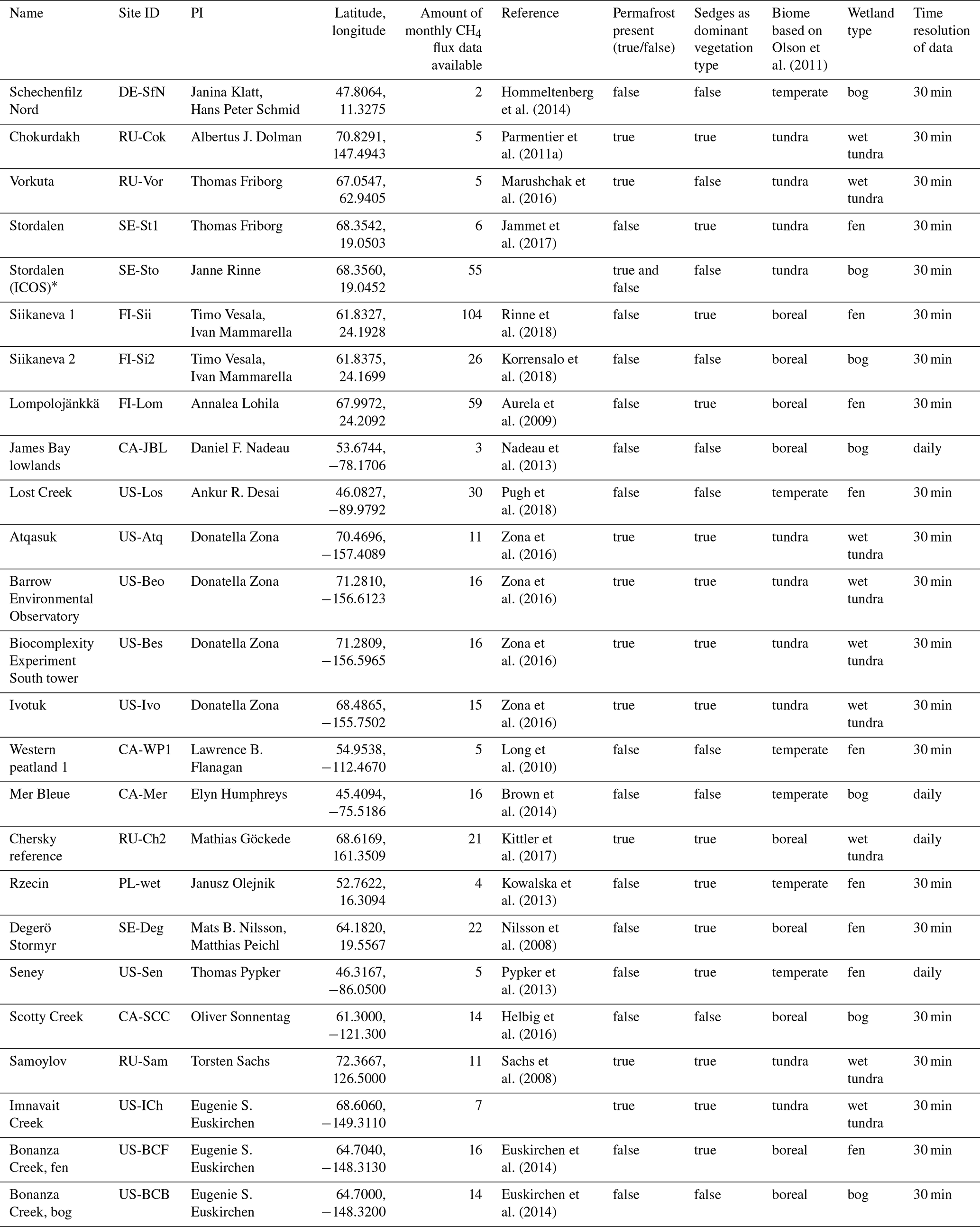
Data were acquired from 25 sites that (1) measure CH4 fluxes with the EC technique, (2) are located north of 45∘ N and (3) are wetlands as defined above and without substantial human influence on ecosystem functioning (see the site locations in Fig. 1 and the site list in Appendix A). The sites were evenly distributed among wetland types, including fens (n=9), bogs (7), and wet tundra (9), as well as among different biomes, including tundra (11), boreal (8), and temperate (6) biomes, as defined in Olson et al., (2001). At 15 of the 25 sites, sedges (e.g. Rhynchospora alba, Eriophorum vaginatum, Carex limosa) were the dominant vascular plant functional type in the flux measurement source area. Most of the sites (18 out of 25) were located north of 60∘ N and the highest densities of sites were in Fennoscandia and Alaska (Fig. 1). The magnitude of monthly CH4 flux data varied between sites and the median time series length was 14.5 months of CH4 flux data per site. Overall, the dataset spanned between 2005 and 2016. The sites represent northern wetlands sufficiently well to create an upscaled CH4 flux product based on EC data. Sites are referred to with their FLUXNET IDs and if these were not available then new temporary site IDs were generated for this study (see Appendix A).
Site principal investigators (PIs) provided CH4 fluxes and their potential drivers (air temperature and pressure, precipitation, wind speed and direction, friction velocity, net ecosystem exchange of CO2 and its components – i.e. canopy photosynthesis and ecosystem respiration – photosynthetically active radiation, water table depth, and soil temperature) . However, out of the in situ measurements only air temperature and precipitation were used for developing the RF model for flux upscaling since gridded data products of the other potentially important drivers were not readily available and/or the data for the other drivers were missing from several sites.
The 30 min averaged flux data were acquired from 21 sites and daily data were provided for 4 sites. The flux time series were quality filtered by removing fluxes with the worst quality flag (based on 0,1,2 flagging scheme, Mauder et al., 2013) and with friction velocity below a site-specific threshold (if friction velocity and threshold were available for the site). After filtering, daily medians were calculated if the daily data coverage was above 29 out of 48 half-hourly data points (daily data coverage at a minimum of 10 data points for sites without a diel pattern in CH4 flux) and no gap filling was done to the time series prior to calculation of daily values. While this may cause slight systematic bias in the daily flux values, this bias is unlikely to be significant because the magnitude of diel patterns in CH4 fluxes is typically moderate (e.g. Long et al., 2010) or negligible (e.g. Rinne et al., 2018), although at sites with Phragmites cover a relatively strong diurnal cycle can be observed (e.g. Kim et al., 1999; Kowalska et al., 2013).
Unlike the CH4 flux data, the other in situ data from the sites were gap filled prior to the calculation of daily values. The gap filling was done only if the daily data coverage was above 60 % and days with lower data coverage, no daily values calculated. Shorter gaps (<2 h) were filled with linear interpolation, whereas longer gaps (between 2 to 14.5 h) were replaced with mean diurnal variation within a 30 d moving window. However, for precipitation, daily sums were calculated without any gap filling. Besides the measurements at the sites, potential solar radiation (Rpot) and its time derivative (der(Rpot)) were calculated based on latitude and time of measurement. In order to remove the Rpot latitudinal dependence it was normalized to be between 0 and 1 before usage.
CH4 flux drivers measured in situ, in addition to the remote-sensing data (Sect. 2.3.2), were used for the gap filling of CH4 time series with the RF algorithm (Sect. 2.1.1). For each site the gap-filling models generally agreed well with the independent validation data (mean NSE =0.74 and mean RMSE =9 nmol m−2 s−1). After gap filling, the CH4 flux time series were aggregated to monthly values if the monthly data coverage prior to gap filling was at least 20 %.
The daily time series of air temperature and precipitation measured at the sites were gap filled using the WATCH Forcing Data methodology applied to ERA-Interim (WFDEI) data (Weedon et al., 2014). Prior to using the WFDEI data for gap filling, the data were bias-corrected for each site as is typically done for climate or weather reanalysis data (e.g. Räisänen and Räty, 2013; Räty et al., 2014). For precipitation, the mean of WFDEI data were simply adjusted to match site mean precipitation. For air temperature, the bias correction was done for each month separately using quantile mapping with smoothing within a moving 7-month window. Quantile mapping compares the cumulative distribution functions (CDFs) of WFDEI and site measurements against each other and adjusts the WFDEI data so that after adjustment its CDF matches with the CDF of the site measurements (e.g. Räisänen and Räty, 2013). After gap filling the daily time series with WFDEI data, monthly and annual precipitation were calculated, in addition to monthly mean air temperature.
2.3.2 Remote-sensing data
Several data products from the Moderate Resolution Imaging Spectrometer (MODIS) were used in this study to derive various driving variables. For RF model development the following data products at 500 or 1000 m spatial resolution were used: MOD10A1 snow cover (Hall and Rigs, 2016), MOD11A2 daytime and night-time land surface temperature (LSTd and LSTn, Wan et al., 2015a), MOD13A3 enhanced vegetation index (EVI, Didan, 2015), and MOD09A1 surface reflectance (Vermote, 2015). More elaborate data products estimating ecosystem gross primary productivity (GPP) and net primary productivity (NPP; MOD17) were not included here for two reasons: (1) many of the sites included here were misclassified in the land cover map used in MOD17 (e.g. as woody savanna), hence severely influencing the estimated GPP and NPP (Zhao et al., 2005), and (2) sites that were correctly classified as permanent wetlands were in fact assigned a fill value and removed from the product since the product is not strictly valid for these areas (Lees et al., 2018). All the remote-sensing data products were quality filtered using the quality flags provided along with the data.
The MODIS snow cover ranged from 0 (no snow) to 100 (full snow cover) and was converted to a simple snow cover flag (SC) consisting of 0 and 1 depending whether the snow cover data were below or above 50, respectively. A vector containing days since snow melt (DSSM) was calculated using the snow cover flag and normalized to 0 (beginning) and 1 (end) for each growing season (Mastepanov et al., 2013). The MOD09A1 surface reflectance at bands 2 (841–876 nm) and 5 (1230–1250 nm) were used to calculate the simple ratio water index (SRWI = band 2/band 5), following Zarco-Tejada and Ustin (2001). SRWI showed spurious values when there was snow cover, and hence these points were replaced with the mean SRWI observed at each site when there was no snow. Meingast et al. (2014) showed that SRWI can be used as a proxy for wetland water table depth, although their results were affected by changes in vegetation cover, which might hinder across-site comparability in this study. Additionally, following the temperature and greenness modelling approach (Sims et al., 2008), a product of EVI and LSTd was included in the analysis as a proxy for GPP, following a previous peatland study (Schubert et al., 2010). The remote-sensing data were provided with daily (MOD10A1), 8 d (MOD09A1, MOD11A2) or monthly (MOD13A3) time resolution and the data were aggregated to monthly means prior to usage.
2.3.3 Additional categorical variables
The sites were also classified based on the presence of permafrost in the source area (present or absent) and according to biome type. Biome types (temperate, boreal and tundra) were determined from Olson et al. (2001) and the information about the permafrost was provided by the site PIs. Furthermore, the data were categorized based on wetland type and sedge cover as in Treat et al. (2018) and Turetsky et al. (2014). However, such information is not available in the gridded format needed for upscaling; nevertheless, inclusion of these variables can be used to assess how much they increase the predictive performance of the model.
2.4 Gridded datasets used in flux upscaling
For upscaling CH4 fluxes using the developed RF model, the LST data were acquired from the aggregated product MOD11C3 (Wan et al., 2015b) and snow cover data from MOD10CM (Hall and Riggs, 2018). Distribution of permafrost in the northern latitudes were estimated using the circum-Arctic map of permafrost derived by National Snow and Ice Data Center (Brown et al., 2002). The resolution of the gridded data was adjusted to match the resolution of the wetland maps using bilinear interpolation if needed. Additionally, land and ocean masks (Jet Propulsion Laboratory, 2013) were utilized when processing the gridded datasets.
2.5 Wetland maps
Upscaled fluxes were initially estimated in flux densities per wetland area, i.e. amount of CH4 per area of wetland per unit of time. To create a gridded product of CH4 emissions from the northern wetlands, these upscaled flux densities were converted into (amount of CH4) per (grid cell area) per (unit of time) using different wetland maps. Wetland mapping is an ongoing field of research and the usage of different wetland maps contributes to the uncertainty of global wetland CH4 emission estimates (e.g. Bloom et al., 2017a; Z. Zhang et al., 2017). Hence, three different wetland maps (PEATMAP, DYPTOP and GLWD) were used in this study to evaluate how much they affect the overall estimates of northern high-latitude wetland CH4 emissions.
The recently developed static wetland map PEATMAP (Xu et al., 2018) combines detailed geospatial information from various sources to produce a global map of wetland extent. Here, the polygons in PEATMAP were converted to fractions of wetland in 0.5∘ grid cells. While PEATMAP is focused on mapping peatlands, marshes and swamps (typically on mineral soil) are included in the product for certain areas in the northern latitudes. However, most of the wetlands in the northern latitudes are peatlands, and thus PEATMAP is suitable for our upscaling purposes. The dynamic wetland map estimated by the DYPTOP model (Stocker et al., 2014) was used by aggregating peat and inundated areas to form one dynamic wetland map with 1∘ resolution. The widely used Global Lakes and Wetlands Database (GLWD, Lehner and Döll, 2004) is a static wetland map with 30 arcsec resolution and since it has been widely used here it provided a point of reference for the other two maps. The map was aggregated to 0.5∘ resolution and lakes, reservoirs and rivers were excluded from the aggregated map.
2.6 Process models
The upscaled CH4 fluxes were compared against the output from two process models: LPX-Bern (Spahni et al., 2013; Stocker et al., 2013; Zürcher et al., 2013) and the model ensemble WetCHARTs version 1.0 (Bloom et al., 2017a, 2017b). LPX-Bern is a dynamic global vegetation model that models carbon and nitrogen cycling in terrestrial ecosystems. The model has a separate peatland module with peatland-specific plant functional types (for more details, see Spahni et al., 2013). The wetland extent in LPX-Bern was dynamically estimated using the DYPTOP approach with 1∘ resolution (Stocker et al., 2014). WetCHARTs combines several prescribed wetland maps with different gridded products for heterotrophic respiration and temperature sensitivity (Q10) parameterizations for CH4 production to form a model ensemble of wetland CH4 emissions (Bloom et al., 2017b). Here we used the extended ensemble of WetCHARTs.
3.1 Selecting the predictors for the RF model
The predictors in Table 1 were selected one by one using the procedure described in Sect. 2.1.2. The order in which the predictors were selected is shown in Fig. 2. LSTn alone gave NSE =0.29. After including the category permafrost presence and absence, Rpot, SC and biome class increased NSE to 0.47. However, the influence of SC and biome class on the model performance was marginal based on the small increase in NSE. Additional predictors did not increase the model performance further because (1) they were strongly correlated with a predictor already included in the model (e.g. Tair is correlated with LSTn) or (2) the predictors did not contain any information about CH4 flux variability. The model response to predictors other than biome category was physically reasonable (e.g. permafrost and snow cover decrease fluxes, close to exponential dependence on LSTn), whereas the response to biome category was contrary to expectations. The RF model estimated the CH4 flux magnitude from the different biomes to be in the following order: tundra < temperate < boreal. However, in prior studies it has been shown to be in the following order: tundra < boreal < temperate (Knox et al., 2019; Treat et al., 2018; Turetsky et al., 2014). This discrepancy may be due to the limited number of measurement sites and related sampling bias problems. Hence, in order not to upscale an incorrect pattern of decreasing CH4 emissions when moving from boreal to temperate regions, the biome class was omitted from upscaling. In the subsequent analysis and flux upscaling only the four first predictors (LSTn, permafrost category, Rpot and SC) are utilized.
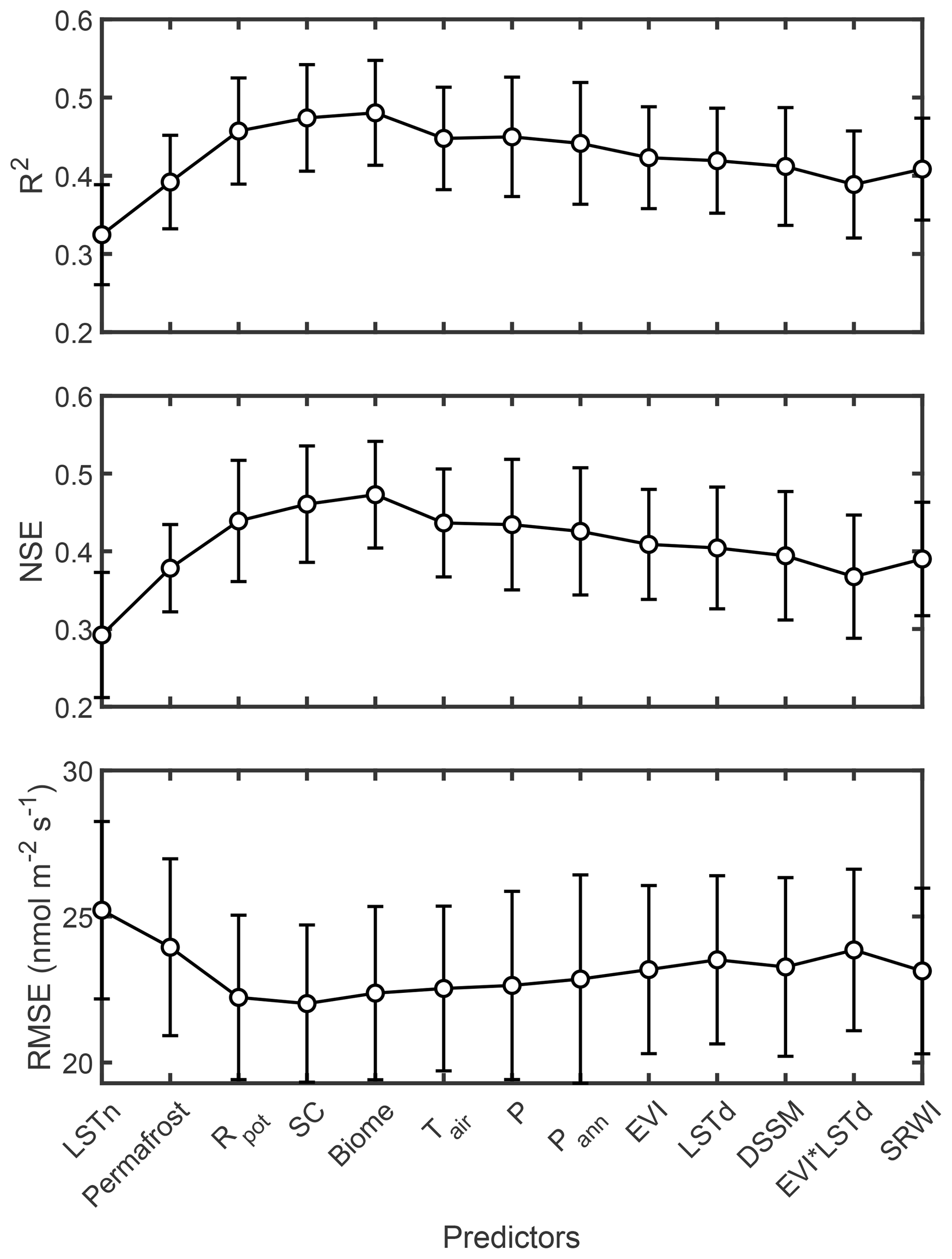
Figure 2Evolution of statistical metrics during RF model development. Predictors were added to the RF model starting from the left of the figure and accumulate along the x axis. For instance, the x tick label “SC” shows the RF model performance when LSTn, Permafrost, Rpot and SC were used as predictors in the model. See the x tick label explanations in Table 1. The error bars denote 1σ uncertainty of the values estimated with bootstrapping.
We further tested whether information about wetland type or sedge cover would improve the model performance even though these categorical variables were not available in gridded format and hence were not usable for upscaling. Including the sedge flag increased the NSE to 0.53, although the increase in Pearson correlation was not statistically significant (p>0.05, comparison of correlation coefficients using Fisher's r to z transformation). Also, wetland type did not have a statistically significant influence on the model performance (p>0.05 and NSE =0.49 if type included). Using too many categorical variables in a RF model may be problematic because each site may end up with a unique combination of categorical variables.
The most important predictor for the model was temperature, similar to numerous studies showing that wetland CH4 emissions are strongly correlated to soil temperature (Christensen et al., 2003; Helbig et al., 2017; Jackowicz-Korczyński et al., 2010; Rinne et al., 2018; Yvon-Durocher et al., 2014; Knox et al., 2019). Selection of LSTn as the primary driver instead of the other temperature variables was likely an outcome of the available data and the algorithm used to select the drivers. With slightly different dataset (more sites) other temperature variables (e.g. Tair) might have been more important drivers for the CH4 flux variability. Estimating apparent Q10 from the RF model LSTn dependence yielded a value of 1.90±0.03 and for validation data it was slightly higher (1.97±0.06) (Fig. 3). These values are comparable to the ones reported in Turetsky et al. (2014) for CH4 chamber measurements at bog and fen sites. The temperature dependence of CH4 production is modelled in many process models with the parameter Q10 value close to 2 (Xu et al., 2016b), which agrees with the CH4 emission temperature dependence shown here. However, one should note that CH4 oxidation also depends on temperature and the derived apparent Q10 value describes the temperature dependence of surface CH4 emission, which is always a combination of CH4 production and oxidation.
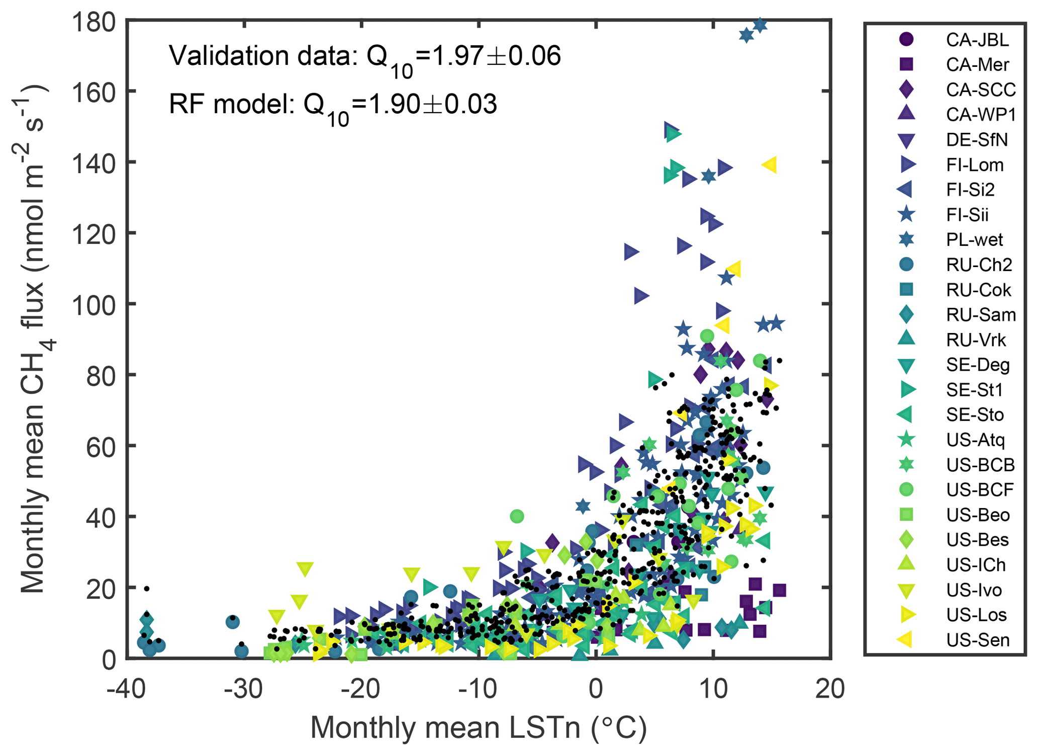
Figure 3Dependence of monthly mean CH4 emissions on monthly mean land surface temperature at night (LSTn) derived from MODIS data. Eddy covariance measurements are shown with filled markers (unique colour for each site) and random forest model predictions for each site are given with black dots.
3.2 Model agreement with validation data
The overall systematic bias (BE) between the RF predictions and validation data was negligible (Fig. 4), whereas the spread of the data (RE) was more pronounced (Fig. 4). Following Moffat et al. (2010), RE was analysed further by binning the data based on CH4 flux magnitude and calculating RE for each bin. RE was clearly correlated with flux magnitude ( nmol m−2 s−1, where FCH4 denotes CH4 flux), indicating that the relative random error of the RF model prediction was nearly constant and approximately 50 % for high fluxes. The systematic error BE did not show a clear dependence on flux magnitude. The RF model performance was worse on a site mean level than with monthly data. When comparing site means, NSE and R2 were both 0.25 and RE and BE were 27.0 and 1.5 nmol m−2 s−1, respectively. Possible drivers causing the remaining CH4 flux variability not captured by the RF model (i.e. the scatter in Fig. 4) are discussed in Sect. 4.2.1.
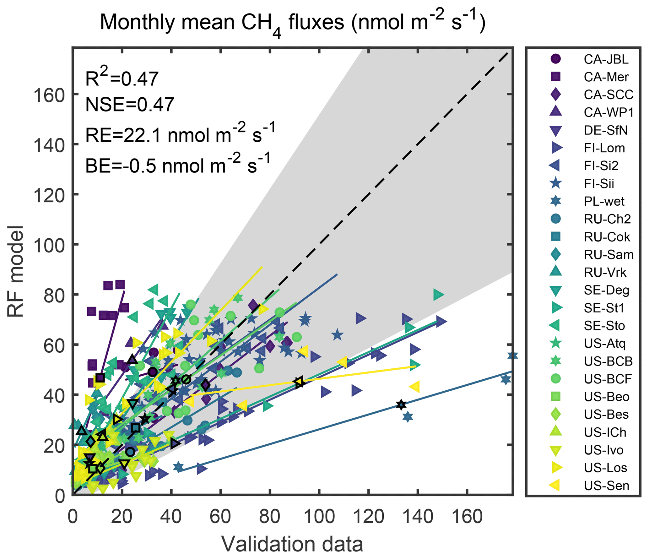
Figure 4Relation between monthly mean CH4 fluxes predicted by the RF model and independent validation data. Monthly average values from the same site are identified by unique colours and a least-squares linear fit to data from each site is also plotted using the same colour. Site means are shown with markers with black edges. The dashed line shows the 1:1 line. The shaded area shows the uncertainty range estimated from the RE CH4 flux dependence (see text for further details). The statistics in the figure are calculated using the monthly data. See Appendix A for an explanation of site names.
When considering the model performance for each site separately, the agreement shows different characteristics (see Fig. 5 for four examples). For individual sites the magnitude of BE is typically somewhat higher (median of absolute value of BE approximately 11 nmol m−2 s−1), whereas RE is lower than for the overall agreement (median RE approximately 10 nmol m−2 s−1). These results indicate that the upscaled CH4 fluxes have, in general, relatively low bias and high random error, whereas individual pixels in the upscaled CH4 map may have higher bias but lower random error.
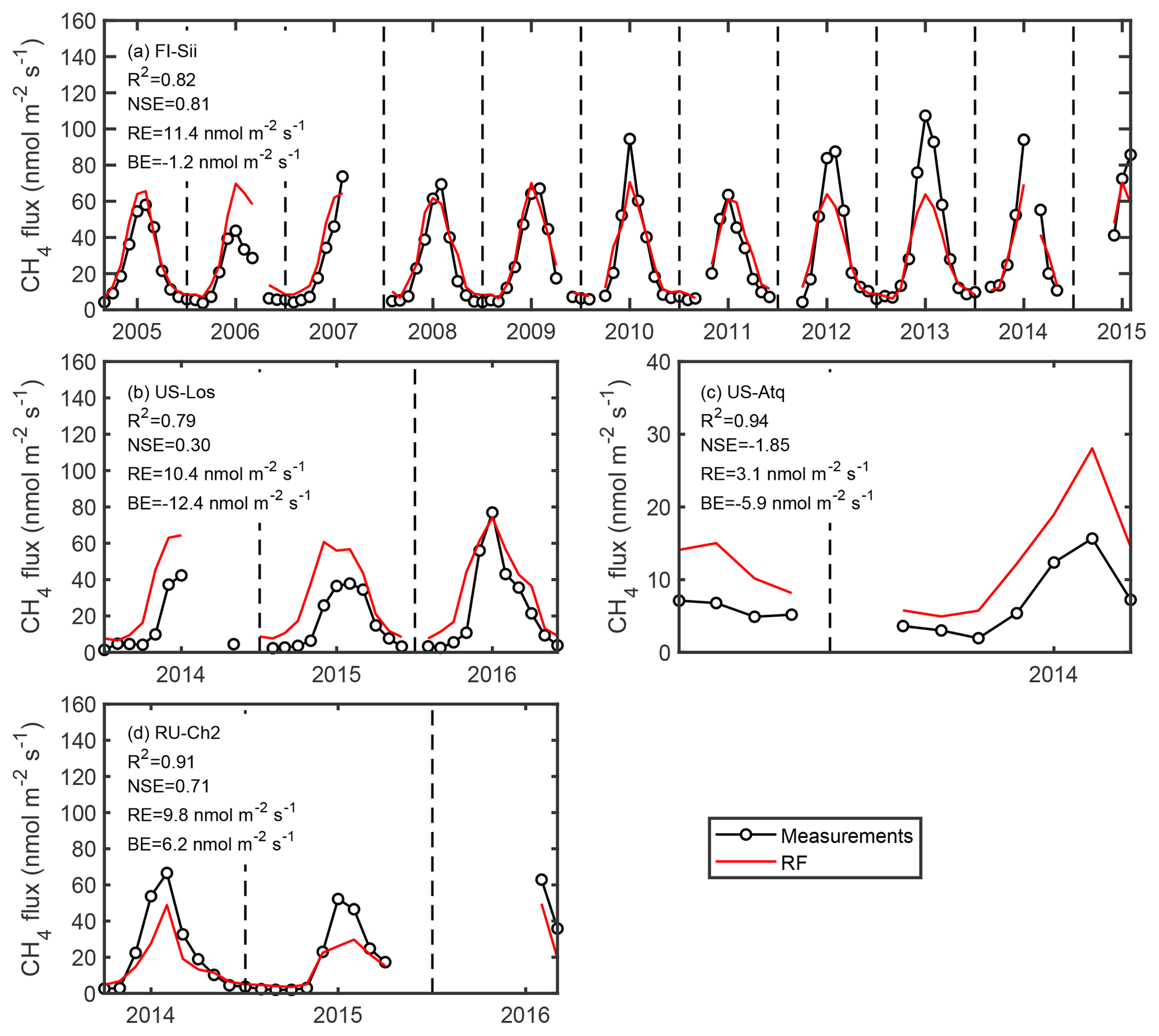
Figure 5Time series of modelled CH4 emissions (red lines) together with validation data (circles) at four example sites: (a) Siikaneva oligotrophic fen in Finland, (b) Lost Creek shrub fen in Wisconsin, USA, (c) Atqasuk wet tundra in Alaska, USA, and (d) Chersky wet tundra in northeastern Siberia, Russia. Dashed vertical lines denote a new year. Note the changes in y axis scales. Site-specific model performance metrics are also included.
The mean annual cycle of CH4 emission predicted by the RF model agrees well with the mean annual cycle calculated from the validation data (not shown). During the non-growing season the RF model slightly overestimates the fluxes (15 % overestimation) but such differences were negligible during the rest of the year (<1 %). However, for individual sites CH4 emission seasonality agrees less. For instance, at US-Los the modelled CH4 emissions start to increase 1 month earlier in the spring (Fig. 5b). The non-growing season fluxes are overestimated at four example sites (FI-Sii, US-Los, US-Atq and RU-Ch2; Fig. 5). The mean flux magnitude is modelled well at FI-Sii (Fig. 5a), whereas at US-Los (Fig. 5b) and US-Atq (Fig. 5c) the RF model overestimates and at RU-Ch2 (Fig. 5d) underestimates the CH4 emissions. The flux bias had a relatively large impact on site-specific NSE. For example, for US-Atq NSE was −1.85, meaning that the observation mean would be a better predictor for this site than the RF model (see the NSE definition in Sect. 2.2). The RF model is not able to replicate the between-year differences in CH4 emissions at the example sites. Capturing interannual variability has also been difficult in previous upscaling studies of CO2 and energy fluxes (e.g. Tramontana et al., 2016).
In general, the RF model performance was better for permafrost-free sites than for sites with permafrost (r=0.66 and r=0.51, respectively; p<0.05), which is likely related to the fact that at sites with permafrost the MODIS LSTn is not as directly related to the soil temperature than at sites without permafrost. Hence, LSTn is not as good proxy for the temperature that is controlling both CH4 production and consumption and this results in a worse performance than at sites without permafrost.
3.3 Upscaled CH4 fluxes
The RF model developed in this study was used together with the gridded input datasets (Sect. 2.4) and wetland distribution maps (Sect. 2.5) to estimate CH4 emissions from northern wetlands in 2013 and 2014. The mean CH4 emissions of the 2 years from the RF model are plotted in Fig. 6 together with CH4 wetland emission maps from the process model LPX-Bern and model ensemble WetCHARTs. Differences between the process model estimations and upscaled fluxes are shown in Fig. 7. In general, the spatial patterns are similar among emission maps, which is not surprising given that the spatial variability is largely controlled by the underlying wetland distributions. One noteworthy difference is that WetCHARTs, RF-PEATMAP (i.e. RF modelling with PEATMAP) and RF-GLWD show higher emissions from western Canada than LPX-Bern or the upscaled fluxes using the wetland map from that process model (RF-DYPTOP). The other difference is that RF-GLWD show negligible emissions from Fennoscandia (Fig. 6c). These differences are related to differences in the underlying wetland maps. While the wetland maps differ, there is no consensus on which is more accurate, so comparisons indicate the uncertainty in upscaling emanating from uncertainties in wetland distribution.
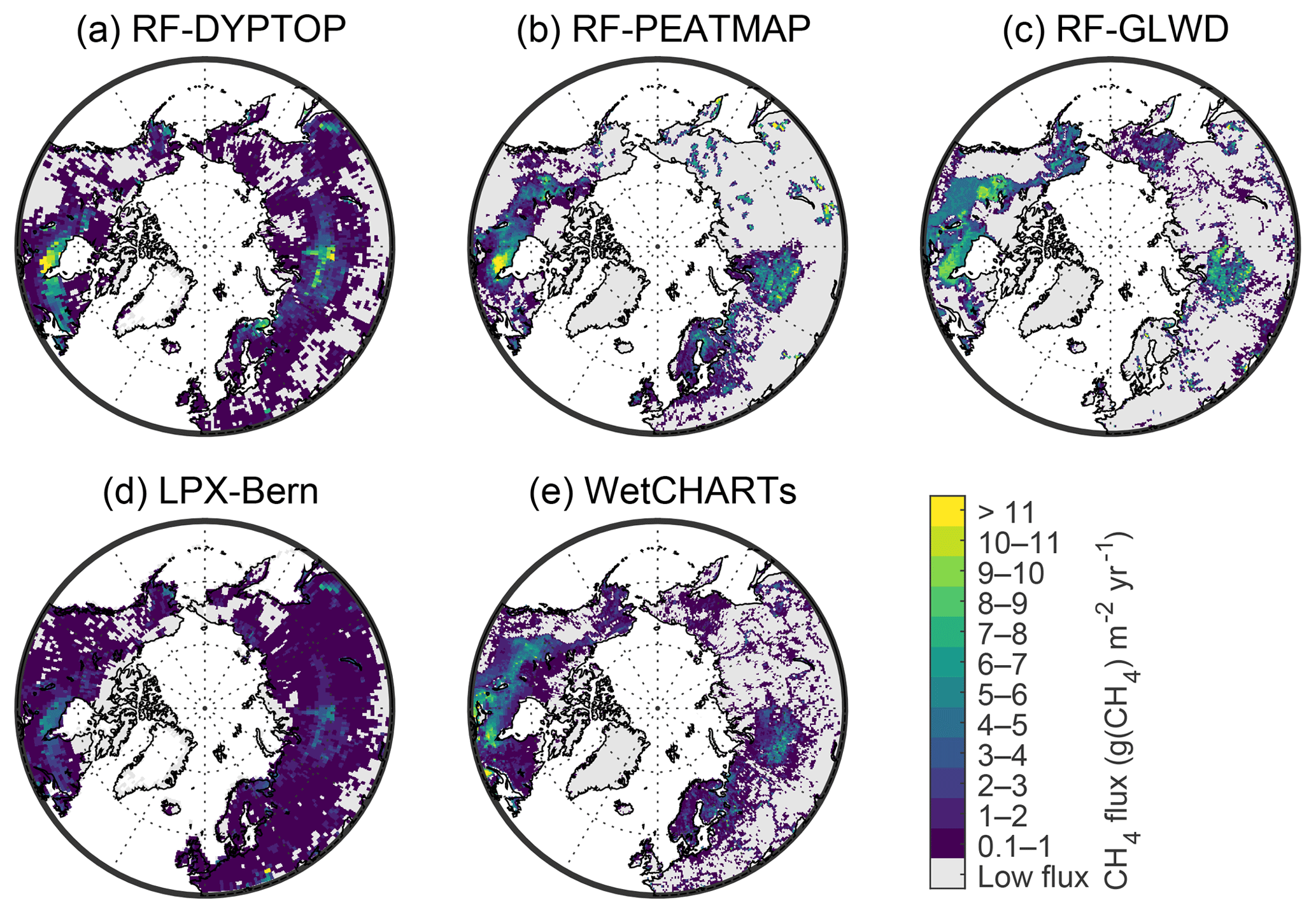
Figure 6Mean annual CH4 wetland emissions during years 2013–2014 estimated by upscaling EC data using the RF model and three wetland maps (a, b, c) and process models (d, e). Grid cells with low CH4 wetland emissions (below 0.1 g(CH4) m−2 yr−1) are shown in grey. The flux rates refer to total unit area in a grid cell.
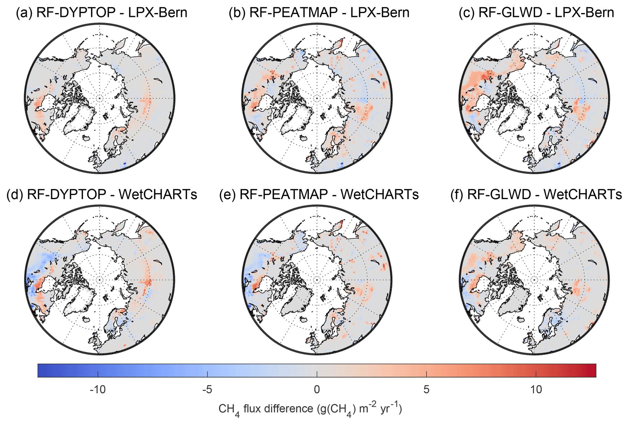
Figure 7Difference in mean annual CH4 wetland emissions during the years 2013–2014 estimated by upscaling EC data using the RF model with different wetland maps and process models. All the CH4 emission maps were aggregated to 1∘ resolution before comparison. The flux rates refer to total unit area in a grid cell.
Three statistical metrics (NSE, R2 and RE) were calculated between RF-DYPTOP and LPX-Bern for each grid cell (Fig. 8). The figure illustrates how well the temporal variability of CH4 emissions estimated by RF-DYPTOP and LPX-Bern agree in each grid cell. NSE values are low in areas where the systematic difference between RF-DYPTOP and LPX-Bern was high (compare Figs. 8a and 7a) since the bias strongly penalizes NSE. The R2 values are high throughout the study domain, likely due to the fact that the seasonal cycle of CH4 emissions dominated the temporal variability in most of the grid cells and the seasonal cycles were in phase between RF-DYPTOP and LPX-Bern. RE values calculated between RF-DYPTOP and LPX-Bern were high in areas where the emissions estimated by RF-DYPTOP were also high (compare Figs. 8c and 6a). This is likely due to the fact that, even though the seasonal cycles were in phase, their amplitudes were different which increased the variability between LPX-Bern and RF-DYPTOP (i.e. increase in RE).
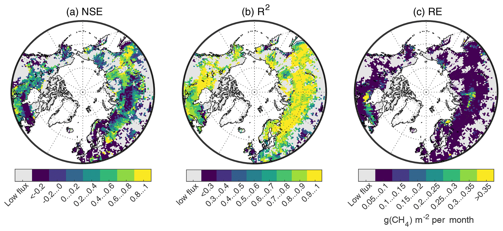
Figure 8NSE, R2 and RE calculated between RF-DYPTOP and LPX-Bern. Grid cells with low CH4 wetland emissions (below 0.1 g(CH4) m−2 yr−1) are shown in grey. RE values refer to total unit area in a grid cell.
The uncertainties of the upscaled fluxes were estimated from the spread of predictions made with the ensemble of 200 RF models (Fig. 9). The uncertainty mostly scales with the flux magnitude (compare Fig. 6a–c with Fig. 9a–c), meaning that grid cells with high fluxes tend to also have high uncertainties. However, the relative flux uncertainty does have some geographical variation (Fig. 9d–f). The highest relative uncertainties are typically at the highest and lowest latitudes of the study domain. In these locations the dependencies between the predictors and the CH4 flux are not as well defined as in the locations with lower uncertainties leading to larger spread in the ensemble of RF model prediction. For instance, at low latitudes LSTn may go beyond the range of LSTn values in the training data (see the range in Fig. 3), and hence the RF model predictions are not well constrained in these situations. On the other hand, lower relative uncertainties are typically obtained for locations close to the measurement sites incorporated in this study (compare Figs. 1 and 9), since the dependencies between the predictors and the CH4 flux are better defined.
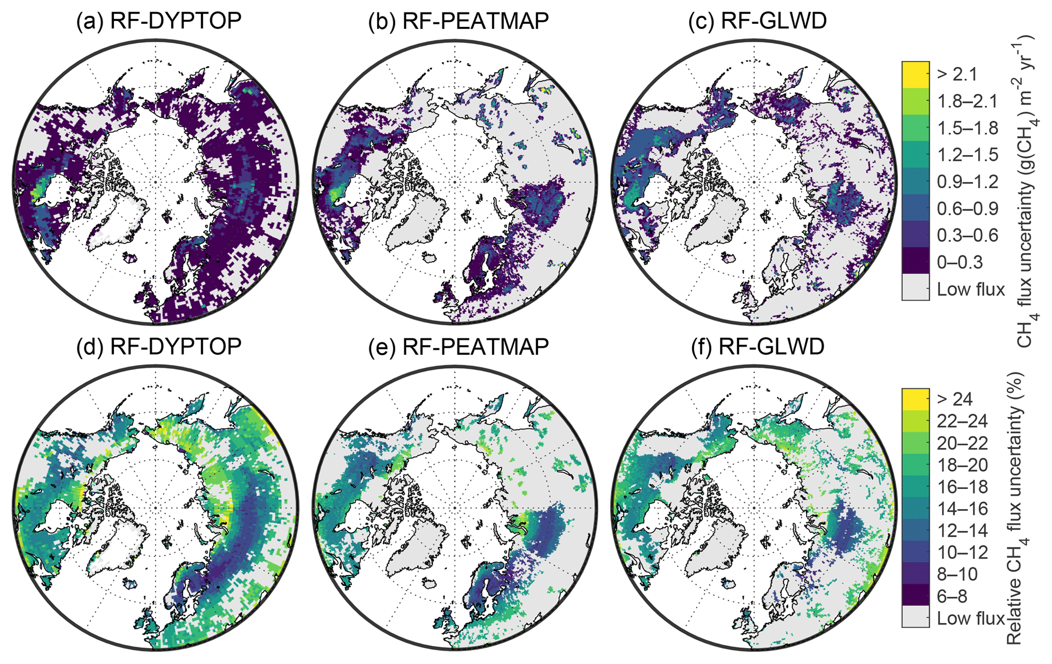
Figure 9Absolute (a–c) and relative (d–f) uncertainties of the upscaled CH4 fluxes using different wetland maps. Uncertainty is estimated as 1σ variability of the predictions by 200 RF models developed by bootstrapping the training data (Sect. 2.1.2). Grid cells with low CH4 wetland emissions (below 0.1 g(CH4) m−2 yr−1) are shown in grey. The absolute uncertainties refer to total unit area in a grid cell.
The seasonalities of the upscaled fluxes and CH4 fluxes from process models are similar with the highest CH4 emissions in July–August and the lowest in February. This seasonal pattern is consistent throughout the study domain (Fig. 10). Warwick et al. (2016) and Thonat et al. (2017) showed that the northern wetland CH4 emissions should peak in August–September in order to correctly explain the seasonality of atmospheric CH4 mixing ratios and isotopes measured across the Arctic. Hence, the wetland CH4 emissions presented here are peaking approximately 1 month too early to perfectly match with their findings. CH4 flux magnitude agrees well between WetCHARTs and the upscaled flux during spring and midsummer (April–July), whereas LPX-Bern estimates lower fluxes (0 % and 26 % difference, respectively). During late summer and autumn (August–October) both process models estimate slightly lower fluxes than the upscaled estimate (17 % and 19 % difference, respectively). The upscaled fluxes also show somewhat higher emissions during the non-growing season (November–March) than the two process models (27 % and 35 % difference; see Table 2), and the upscaled estimates of non-growing season emissions are relatively close to a recent model estimate (Treat et al., 2018). This result promotes the recent notion that process models might be underestimating non-growing season fluxes at high latitudes (e.g. Treat et al., 2018; Xu et al., 2016a; Zona et al., 2016).

Figure 10Monthly time series of zonal mean CH4 fluxes. The upscaled fluxes with different wetland maps are shown in (a, b, c) and wetland CH4 emissions estimated with the two process models are given in (d, e).
Table 2Annual CH4 wetland emissions in different subdomains (Hudson Bay lowlands and western Siberian lowlands; see Fig. 1) and time periods. The values are given in Tg(CH4) yr−1. Note that estimates from some reference studies are not for the same period as the one studied here (2013–2014). For WetCHARTs the mean of the model ensemble together with the range (in parentheses) is given, whereas for the upscaling results the 95 % confidence intervals for the estimated emissions are given.
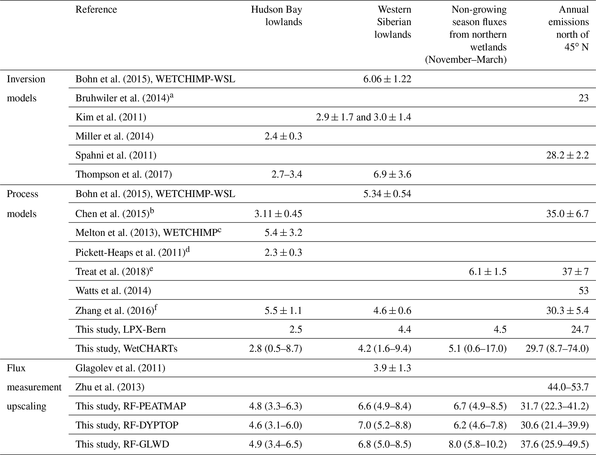
a Approximately north of 47∘ N. b Approximately north of 45∘ N. c Mean annual CH4 emissions from eight models ±1σ of interannual variation in the model estimates for the period 1993–2004. d Process model tuned to match atmospheric observations. e North of 40∘ N. f Mean ±1σ over the LPJ-wsl model results using different wetland extents for the period 1980–2000.
Treat et al. (2018) adjusted WetCHARTs model output so that it matches with their estimates of non-growing season CH4 emissions and then estimated annual wetland CH4 emissions north of 40∘ N to be 37±7 Tg(CH4) yr−1 using this adjusted model output. The estimates derived here for the annual emissions using the three wetland maps are similar (see Table 2), especially when considering our slightly smaller study domain (above 45∘ N). The two process models included in this study estimated slightly lower mean annual emissions than the upscaled fluxes (11 % and 26 % difference between the mean upscaled estimate and WetCHARTs and LPX-Bern, respectively; see also Table 2). However, given the uncertainties in upscaling as well as in process models, this can be regarded as relatively good agreement. Different process models may be driven with different climate forcing data and they may have discrepancies in the underlying wetland distributions, in addition to the different parameterizations and descriptions of the processes behind the CH4 emissions. These sources of uncertainty should be recognized when models are compared against each other or against upscaling products.
In order to further evaluate the agreement between the upscaled fluxes and process models we focused on two specific regions: Hudson Bay lowlands (HBL) and western Siberian lowlands (WSL) (see locations in Fig. 1). The upscaled fluxes indicate higher annual emissions for both subdomains compared to the two process models or previously published estimate (Table 2). For WSL the upscaled estimates are within the range of variability observed between process models and inversion modelling in WETCHIMP-WSL (Bohn et al., 2015) and close to Thompson et al. (2017). The upscaled estimates by Glagolev et al. (2011) might underestimate CH4 emissions from the WSL area (Bohn et al., 2015). Furthermore, the process models in Bohn et al. (2015) are likely underestimating the non-growing season CH4 emissions which might partly explain the discrepancy to the upscaled estimates in this study. Hence, the upscaled CH4 emission estimates for the WSL area, while large, are still in a reasonable range.
For HBL, the discrepancy between upscaled emission estimates and the estimates based on process models or previous studies is larger (Table 2). The upscaling results agree with Zhang et al. (2016) and Melton et al. (2013) but show emissions that are twice as large for the HBL than the other estimates (Table 2). This cannot be explained by wetland mapping since the difference also holds when the DYPTOP wetland map is used in upscaling. There are only few long-term EC flux studies conducted in the HBL area and the only one found (Hanis et al., 2013) showed on average 6.9 g(CH4) m−2 annual emissions at a subarctic fen located in the HBL. If the upscaled CH4 emissions are downscaled back to ecosystem level in the HBL area with wetland maps, we get on average 11.0 g(CH4) m−2 annual CH4 emission for the HBL area based on the RF model output, which is 1.6 times larger than the estimate by Hanis et al. (2013). While Hanis et al. (2013) studied only one wetland during different years than those used here (years 2008–2011 in Hanis et al., 2013, here 2013–2014), it is still noteworthy that the relative difference between Hanis et al. (2013) and this study is similar to the discrepancy between this study and the inversion estimates (Pickett-Heaps et al., 2011; Thompson et al., 2017) at the whole HBL scale. Pickett-Heaps et al. (2011) and Thompson et al. (2017) show near zero CH4 emissions during October–April and onset of CH4 emissions in mid-May or even June, largely dependent on when the ground was free of snow and unfrozen. This is somewhat surprising given the fact that only 32 % of wetlands in the area are underlain by permafrost (based on amalgam of PEATMAP and the permafrost map), and hence the soils are likely not completely frozen and some non-growing season CH4 emissions are likely to occur in such conditions (e.g. Treat et al., 2018). The upscaled non-growing season CH4 emissions show on average 1.1 Tg(CH4) yr−1 emissions for the HBL area. This partly, but not completely, explains the discrepancy between the CH4 emission estimates for the HBL area. All these results suggest that the upscaled product likely overestimates CH4 emissions from the HBL area.
4.1 Comparing the RF model predictive performance to previous studies
The RF model performance was worse when compared against independent validation data than what has been achieved in previous upscaling studies for GPP and energy fluxes (R2>0.7) and ecosystem respiration (Reco; R2>0.6) (e.g. Jung et al., 2010; Tramontana et al., 2016). However, the RF model performance for monthly CH4 emissions was comparable to net ecosystem exchange of CO2 (NEE) (R2<0.5) (e.g. Jung et al., 2010; Tramontana et al., 2016). Likely reasons for this finding include, for instance, that for other fluxes there is simply more data available from several sites spanning the globe. For example, the La Thuile synthesis dataset used by Jung et al. (2010) and Tramontana et al. (2016) consists of 965 site years of data from over 252 EC stations. Here we have data from 25 sites with CH4 fluxes. Furthermore, the drivers (or proxies for the drivers) of, for example, GPP and energy fluxes are more easily available from remote-sensing (e.g. MODIS) and weather forecasting re-analysis datasets (e.g. WFDEI). In contrast, CH4 emissions are more related to below-ground processes, thus drivers for these processes are more difficult to measure remotely. Also, there are temporal lags between changes in drivers (e.g. LSTn) and CH4 fluxes in response to these changes. Consequently, training a machine-learning model such as RF on such data is difficult since the RF model assumes a instantaneous relationship between the change and response. However, one should also note that GPP or Reco are never directly measured with the EC technique, they are always at least partly derived products (Lasslop et al., 2009; Reichstein et al., 2005). Hence, direct functional relationships between GPP and Reco and their environmental drivers are inherently included in these flux estimates, whereas NEE and CH4 emissions are directly measured without additional modelling. Also, both NEE and CH4 emissions are differences between component fluxes (NEE: GPP and Reco; CH4 flux: production and oxidation). Therefore, GPP and Reco upscaling algorithms show better correspondence with validation data than for NEE or CH4 emissions and the results for NEE would be the correct point of reference for the RF model performance presented here.
While the RF model performance in this study was inferior to previous upscaling studies for other fluxes when evaluated using different statistical metrics, it was still comparable to what has been shown before for several process models for CH4 emissions (McNorton et al., 2016; Wania et al., 2010; Zürcher et al., 2013; Zhu et al., 2014; Xu et al., 2016a). For instance, McNorton et al. (2016) validated the land surface model JULES against CH4 flux data from 13 sites and found R2=0.10 between the validation data and the model. Wania et al. (2010) found on average RMSE =29 nmol m−2 s−1 and RMSE =42 nmol m−2 s−1 with and without tuning their model LPJ-WHyME against CH4 flux data from seven sites, respectively. Zürcher et al. (2013) found the time-integrated CH4 flux to be well represented by LPX-Bern model across different sites. A tight correlation (R2=0.92) is found between simulated and measured cumulative site emissions after calibrating the model against the measurements. While Xu et al. (2016a) did not explicitly show any statistical metrics, their model (CLM4.5) comparison against site level CH4 flux data seemed to be somewhat better than in Wania et al. (2010) or McNorton et al. (2016). Xu et al. (2016a) emphasize the importance of non-growing season emissions and the fact that their model was clearly underestimating these emissions. Zhu et al. (2014) calibrated their model (TRIPLEX-GHG) for each measurement site by changing, e.g. the Q10 for CH4 production and CH4 to CO2 release ratio to be site-specific and found on average R2=0.64 when comparing the calibrated model against measurements at 17 CH4 flux measurement sites. However, their findings are not directly comparable to the RF model agreement with validation data shown here due to their model calibration against data before comparison. Nevertheless, their results show that, even after calibration, the process models are not fully able to capture the CH4 flux variability in measurements. Miller et al. (2014) argued that the structure of some of the process models is so complex that the required forcing variables may not be reliable at larger spatial scales. All of these five models (JULES, LPJ-WHyME, LPX-Bern, CLM4.5 and TRIPLEX-GHG) are contributing to the global CH4 budget estimation within the Global Methane Project (Saunois et al., 2016), highlighting that these results summarize the agreement between state-of-the-art process models and field measurements.
4.2 Methods to improve RF model predictive performance
4.2.1 Missing predictors
In this study a statistical model was developed using the RF algorithm, and the model was able to yield R2=0.47 against monthly CH4 flux validation data. Our upscaling using the RF model focused on 2013–2014, as these were the years with the largest overlap of collected data. However, all data from all the years (2005–2016) were used to develop and validate the model. The incomplete match between the RF model and validation data is likely caused by the fact that not all the possible drivers causing inter- and intra-site variability in CH4 emissions were included in the analysis, and hence all the variability could not be explained by the model.
Christensen et al. (2003) were able to explain practically all the variability (R2=0.92) in annual CH4 emissions in their multi-site chamber study with only two predictors: temperature and the availability of substrates for CH4 production. Also, Yvon-Durocher et al. (2014) speculate that the amount of substrates for microbial CH4 production explains across-site variability of CH4 fluxes in their data. However, gridded data on spatially explicit substrate information are currently nonexistent. Hence, proxies for the substrates available for methanogenesis are needed. The current paradigm on wetland CH4 emissions is that most of the emitted CH4 is produced from recently fixed carbon being used as precursors for the CH4-producing Archaea (e.g. Chanton et al., 1995; Whiting and Chanton, 1993). Most process models are based on the premise that a certain fraction of ecosystem net primary productivity (NPP) is available and used for CH4 production or alternatively a fraction of heterotrophic respiration is allocated to CH4 emissions (e.g. Xu et al., 2016b). Thus, NPP (or GPP) could potentially be included as a predictor for the RF model and used as a proxy for the amount of substrates available for CH4 production. However, the RF model performance in this study was not enhanced if variables closely related to NPP (EVI and the product of EVI and LSTd) were included as predictors. Also, Knox et al. (2019) did not find GPP as an important predictor of CH4 emission variability in their multi-site synthesis study.
Using NPP (or proxies for it) for the RF model development might be an oversimplification, since it has been shown that the deep-rooted sedges and their NPP are especially important for CH4 production (Joabsson and Christensen, 2002; Ström et al., 2003, 2012; Waddington et al., 1996). Hence, information about plant functional types (PFTs) would be needed to better explain the CH4 flux variability (Davidson et al., 2017; Gray et al., 2013). Furthermore, the fraction of the fixed carbon allocated to the roots and released as root exudates (hence, available for CH4 production) varies between species and root age (Proctor and He, 2017; Ström et al., 2003), further complicating the connection between NPP and CH4 emissions. The sedges also act as conduits for CH4, allowing the CH4 produced below water level to rapidly escape to the atmosphere and bypass the oxic zone in which the CH4 might have otherwise been oxidized (Waddington et al., 1996; Whiting and Chanton, 1992). Besides sedges, Spaghnum mosses are also important because methanotrophic bacteria that live in symbiosis with these mosses significantly decrease the CH4 emissions to the atmosphere when they are present (Larmola et al., 2010; Liebner et al., 2011; Parmentier et al., 2011b; Raghoebarsing et al., 2005; Sundh et al., 1995). In a modelling study, Li et al. (2016) showed that it was essential to consider the vegetation differences between sites when modelling CH4 emissions from two northern peatlands. Hence, ideally one should have gridded information on wetland species composition and associated NPP across the high latitudes to significantly improve the upscaling results. Unfortunately, such information is not yet available and therefore modelled estimates could be used (e.g. LPX-Bern, which includes several peatland-specific PFTs allowed to freely evolve during the model run) (Spahni et al., 2013). However, in such cases the upscaled CH4 emission estimates would no longer be independent of the model and therefore would be less suitable for model validation. We also note that many process models have only one PFT per wetland.
Different variables related to water input to the ecosystem (i.e. P, Pann) or surface moisture (SRWI) did not enhance the RF model predictive performance, not only reflecting that water table depth (WTD) is not solely controlled by input of water via precipitation but also that evapotranspiration and lateral flows affect wetland WTD, data that were missing from our study. These findings are consistent with previous studies (e.g. Christensen et al., 2003; Rinne et al., 2018; Pugh et al., 2018 and Knox et al., 2019), who showed only a modest CH4 flux dependence on WTD in wetlands and peatlands. In contrast, several chamber-based studies have shown a positive relationship between WTD and CH4 fluxes (Granberg et al., 1997; Olefeldt et al., 2012; Treat et al., 2018; Turetsky et al., 2014). In general, chamber-based studies often show spatial dependency of CH4 flux on WTD, whereas studies done at an ecosystem scale with EC generally do not show temporal WTD dependency, albeit there are exceptions (e.g. Zona et al., 2009). This might indicate that WTD controls metre-scale spatial heterogeneity of CH4 flux between microtopographical features (e.g. Granberg et al., 1997) but not temporal variability on the ecosystem scale, provided that WTD stays relative close to the surface. Also, the chamber studies tend to observe spatial variation, which can be indirectly influenced by WTD via its influence on plant communities, whereas EC studies observe typically temporal variation in sub-annual timescales. However, the effect of WTD might be masked by a confounding effect caused by plant phenology, since vegetation biomass often peaks at the same time as the WTD is at its lowest. While the variables related to WTD did not increase the RF model performance, WTD might still play a role in controlling ecosystem-scale CH4 variability when it is exceptionally high or low. For instance, the year 2006 was exceptionally dry at the Siikaneva fen, and hence CH4 emissions during that year were lower than on average (see Fig. 5a). However, in order to accurately capture such dependencies with machine-learning techniques (such as RF), they should be frequent enough so that the model can learn these dependencies.
RF model performance was better at permafrost-free than at sites with permafrost, which might indicate that the LSTn might not be an appropriate proxy for the temperature controlling the CH4 production and oxidation rates at sites with permafrost. Also, no information on the development of the seasonally unfrozen, hydrologically and biogeochemically active layer was included in the RF model. Furthermore, Zona et al. (2016) showed strong hysteresis between soil temperatures and CH4 emissions at their permafrost sites in Alaska, whereas Rinne et al. (2018) show a synchronous exponential dependence between soil temperature and CH4 emissions at a boreal fen without permafrost. The hysteresis observed in Zona et al. (2016) could be explained by the fact that part of the produced CH4 at these permafrost sites is stored below ground for several months before it is being emitted to the atmosphere, causing a temporal lag between soil temperature and observed surface flux. In any case, more knowledge of soil processes (soil thawing and freezing, CH4 production and storage) is needed before the CH4 emissions from these permafrost ecosystems can be extrapolated to other areas with greater confidence.
It should be emphasized that the drivers causing across-site variability in ecosystem-scale CH4 emissions are, in general, unknown since studies comparing EC CH4 fluxes from multiple wetland sites have only recently been published (Baldocchi, 2014; Knox et al., 2019; Petrescu et al., 2015). Most previous CH4 synthesis studies were based on plot-scale measurements (Bartlett and Harriss, 1993; Olefeldt et al., 2012; Treat et al., 2018; Turetsky et al., 2014). However, the CH4 flux responses to environmental drivers and their relative importance might be different at an ecosystem scale since CH4 fluxes typically show significant spatial variability at sub-metre scale (e.g. Sachs et al., 2010). Furthermore, the temporal coverage of plot-scale measurements with chambers is usually relatively poor, whereas EC measurements provide continuous data on ecosystem scale. This study and Knox et al. (2019) show that temperature is important when predicting CH4 flux variability in a multi-site CH4 flux dataset, but a significant fraction of CH4 flux variability is still left unexplained. It remains a challenge for future EC CH4 flux synthesis studies to discover the drivers explaining the rest of the variability.
4.2.2 Quality and representativeness of CH4 flux data
The RF model performance may improve if instrumentation, measurement setup and the data processing are harmonized across sites, since these discrepancies between flux sites might have caused spurious differences in CH4 fluxes. These differences would have created additional variability in the synthesis dataset, which would in turn (1) influence the training of RF model and (2) decrease, for example, NSE values obtained against validation data, since there would be artificial variability in the validation data, which is not related to the predictors. In this study, the site PIs processed the data themselves using different processing codes, albeit the gap filling was done centrally in a standardized way.
While these issues mentioned above could impact the upscaling results shown here, prior studies have shown that the usage of different instruments or processing codes does not significantly impact CH4 flux estimates. For instance, Mammarella et al. (2016) showed that the usage of different processing codes (EddyPro and EddyUH) resulted, in general, in a 1 % difference in long-term CH4 emissions. On the other hand, CH4 instrument cross comparisons have shown small differences (typically less than 7 %) between the long-term CH4 emission estimates derived using different instruments (Goodrich et al., 2016; Peltola et al., 2013, 2014). While these studies show consistent CH4 emissions, they also stress that the data should be carefully processed to achieve such good agreement across processing codes and instruments. In addition, many issues related to, for example, friction velocity filtering and gap filling of CH4 fluxes are still unresolved, and the role of short-term emission bursts, which are common in methane flux time series, needs to be further investigated (e.g. Schaller et al., 2017). However, recently Nemitz et al. (2018) advanced these issues by proposing a methodological protocol for EC measurements of CH4 fluxes used to standardize CH4 flux measurements within the ICOS measurement network (Franz et al., 2018).
A total of 25 flux measurement sites were included in this study and they were distributed across the Arctic boreal region (see Fig. 1). The measurements were largely concentrated in Fennoscandia and Alaska, whereas data from, for example, the HBL and WSL areas, were missing. Long-term EC CH4 flux measurements are largely missing from these vast wetland areas, casting uncertainty on wetland CH4 emissions from these areas. The location of a flux site is typically restricted by practical limitations related to, for example, ease of access and availability of grid power. Hence, open-path instruments with low power requirements potentially open up new areas for flux measurements (McDermitt et al., 2010), yet they need continuous maintenance, which is not necessarily easy in remote locations. However, one could argue that the geographical location of flux sites is not vital for upscaling, more important is that the available data represents well the full range of CH4 fluxes across the northern latitudes and more importantly the CH4 flux responses to the environmental drivers. Also, sites should ideally cover all different wetlands with varying plant species composition, whereas geographical representation is not necessarily as important. CH4 flux site representativeness could be potentially assessed in the same vein as in previous studies for other measurement networks (Hargrove et al., 2003; Hoffman et al., 2013; Papale et al., 2015; Sulkava et al., 2011). However, before such analysis can be done, the main drivers causing across-site variability in ecosystem-scale CH4 fluxes should be better identified.
Most of the CH4 flux data here and in the literature have been recorded during the growing season when the CH4 fluxes are at a maximum, whereas year-round continuous CH4 flux measurements are not as common. This is likely due to the harsh conditions in the Arctic during winter that make continuous high-quality flux measurements very demanding (e.g. Goodrich et al., 2016; Kittler et al., 2017a) but also in part since the large-scale importance of non-growing season emissions has just recently been recognized (Kittler et al., 2017b; Treat et al., 2018; Xu et al., 2016a; Zona et al., 2016). For upscaling year-round CH4 emissions, continuous measurements are vital to accurately constrain also the non-growing season emissions and their drivers.
The presented upscaled CH4 flux maps (RF-DYPTOP, RF-PEATMAP and RF-GLWD), their uncertainties and the underlying CH4 flux densities are accessible via an open-data repository Zenodo (Peltola et al., 2019). The datasets are saved in netCDF files and they are accompanied by a readme file. The dataset can be downloaded from https://doi.org/10.5281/zenodo.2560163.
Methane (CH4) emission data comprising over 40 site years from 25 eddy covariance flux measurement sites across the Arctic boreal region were assembled and upscaled to estimate CH4 emissions from northern (>45∘ N) wetlands. The upscaling was done using the random forest (RF) algorithm. The performance of the RF model was evaluated against independent validation data utilizing the leave-one-site-out scheme, which yielded value of 0.47 for both the Nash–Sutcliffe model efficiency and R2. These results are similar to previous upscaling studies for the net ecosystem exchange of carbon dioxide (NEE) but worse for the individual components of NEE or energy fluxes (e.g. Jung et al., 2010; Tramontana et al., 2016). The performance is also comparable to studies where process models are compared against site CH4 flux measurements (McNorton et al., 2016; Wania et al., 2010; Zürcher et al., 2013; Zhu et al., 2014; Xu et al., 2016a). Hence, despite the relatively high fraction of unexplained variability in the CH4 flux data, the upscaling results are useful for comparing against models and could be used to evaluate model results. The three gridded CH4 wetland flux estimates and their uncertainties are openly available for further usage (Peltola et al., 2019).
The upscaling to the regions >45∘ N resulted in mean annual CH4 emissions comparable to prior studies on wetland CH4 emissions from these areas (Bruhwiler et al., 2014; Chen et al., 2015; Spahni et al., 2011; Treat et al., 2018; Watts et al., 2014; Zhang et al., 2016; Zhu et al., 2013) and hence, in general, support the prior modelling results for the northern wetland CH4 emissions. When compared to two validation areas, the upscaling likely overestimated CH4 emissions from the Hudson Bay lowlands, whereas emission estimates for the western Siberian lowlands were in a reasonable range. Future CH4 flux upscaling studies would benefit from long-term continuous CH4 flux measurements, centralized data processing and better incorporation of CH4 flux drivers (e.g. wetland vegetation composition and carbon cycle) from remote-sensing data needed for scaling the fluxes from the site level to the whole Arctic boreal region.
Table A1Description of eddy covariance sites included in this study.
* Data from this site is divided into two since data from two wind directions differ from each other (with and without permafrost).
OP, TA and TV designed the study and YG contributed further ideas for the study. OP did the data processing and analysis. OR prepared the PEATMAP map for the study. PA, MA, BC, ARD, AJD, ESE, TF, MG, MH, EH, GJ, JK, NK, LK, AL, IM, DFN, MBN, WCO, MP, TP, WQ, JR, TS, MS, HPS, OS, CW and DZ provided CH4 fluxes and other in situ data for the study. FJ and SL did the LPX-Bern model runs. OP wrote the first version of the manuscript and all authors provided input.
The authors declare that they have no conflict of interest.
Lawrence B. Flanagan is acknowledged for providing data from CA-WP1 site. Lawrence B. Flanagan acknowledges support from the Natural Sciences and Engineering Council of Canada and Canadian Foundation for Climate and Atmospheric Sciences. Olli Peltola is supported by the postdoctoral researcher project (decision 315424) funded by the Academy of Finland. Olle Räty is supported by the Academy of Finland IIDA-MARI project (decision 313828). Financial support from the Academy of Finland Centre of Excellence (grant nos. 272041 and 307331), Academy Professor projects (grant nos. 312571 and 282842), ICOS-Finland (grant no. 281255) and CARB-ARC project (grant no. 285630) is acknowledged. Sara H. Knox and Robert B. Jackson acknowledge support from the Gordon and Betty Moore Foundation through grant GBMF5439 “Advancing Understanding of the Global Methane Cycle”. Ankur R. Desai acknowledges support of the DOE Ameriflux Network Management Project. Albertus J. Dolman acknowledges support from the Netherlands Earth System Science Centre, NESSC). Torsten Sachs was supported by the Helmholtz Association of German Research Centres (grant no. VH-NG-821). Ivan Mammarella and Timo Vesala thank the EU for supporting the RINGO project funded by the Horizon 2020 Research and Innovation Programme (grant no. 730944). The EU-H2020 CRESCENDO project (grant no. 641816) is also acknowledged. Fortunat Joos and Sebastian Lienert are thankful for support from the Swiss National Science Foundation (grant no. 200020_172476). Mats B. Nilsson and Matthias Peichl acknowledge support from the National Research Council (VR 2018-03966) SITES and ICOS-Sweden.
This research has been supported by the Academy of Finland (grant nos. 315424, 313828, 312571, 282842, 281255, 285630, 272041 and 307331), the Gordon and Betty Moore Foundation (grant no. GBMF5439), the Helmholtz Association (grant no. VH-NG-821), and Horizon 2020 (RINGO (grant no. 730944) and CRESCENDO (grant no. 641816)).
This paper was edited by David Carlson and reviewed by two anonymous referees.
Aalto, J., Karjalainen, O., Hjort, J., and Luoto, M.: Statistical Forecasting of Current and Future Circum-Arctic Ground Temperatures and Active Layer Thickness, Geophys. Res. Lett., 45, 4889–4898, https://doi.org/10.1029/2018GL078007, 2018.
Aurela, M., Lohila, A., Tuovinen, J.-P., Hatakka, J., Riutta, T., and Laurila, T.: Carbon dioxide exchange on a northern boreal fen, Boreal Environ. Res., 14, 699–710, 2009.
Baldocchi, D.: Measuring fluxes of trace gases and energy between ecosystems and the atmosphere – the state and future of the eddy covariance method, Glob. Change Biol., 20, 3600–3609, https://doi.org/10.1111/gcb.12649, 2014.
Bartlett, K. B. and Harriss, R. C.: Review and assessment of methane emissions from wetlands, Chemosphere, 26, 261–320, https://doi.org/10.1016/0045-6535(93)90427-7, 1993.
Beer, C., Reichstein, M., Tomelleri, E., Ciais, P., Jung, M., Carvalhais, N., Rödenbeck, C., Arain, M. A., Baldocchi, D., Bonan, G. B., Bondeau, A., Cescatti, A., Lasslop, G., Lindroth, A., Lomas, M., Luyssaert, S., Margolis, H., Oleson, K. W., Roupsard, O., Veenendaal, E., Viovy, N., Williams, C., Woodward, F. I., and Papale, D.: Terrestrial Gross Carbon Dioxide Uptake: Global Distribution and Covariation with Climate, Science, 329, 834–838, https://doi.org/10.1126/science.1184984, 2010.
Bergamaschi, P., Houweling, S., Segers, A., Krol, M., Frankenberg, C., Scheepmaker, R. A., Dlugokencky, E., Wofsy, S. C., Kort, E. A., Sweeney, C., Schuck, T., Brenninkmeijer, C., Chen, H., Beck, V., and Gerbig, C.: Atmospheric CH4 in the first decade of the 21st century: Inverse modeling analysis using SCIAMACHY satellite retrievals and NOAA surface measurements, J. Geophys. Res.-Atmos., 118, 7350–7369, https://doi.org/10.1002/jgrd.50480, 2013.
Bloom, A. A., Bowman, K. W., Lee, M., Turner, A. J., Schroeder, R., Worden, J. R., Weidner, R., McDonald, K. C., and Jacob, D. J.: A global wetland methane emissions and uncertainty dataset for atmospheric chemical transport models (WetCHARTs version 1.0), Geosci. Model Dev., 10, 2141–2156, https://doi.org/10.5194/gmd-10-2141-2017, 2017a.
Bloom, A. A., Bowman, K. W., Lee, M., Turner, A. J., Schroeder, R., Worden, J. R., Weidner, R. J., McDonald, K. C., and Jacob, D. J.: CMS: Global 0.5-deg Wetland Methane Emissions and Uncertainty (WetCHARTs v1.0), ORNL DAAC, Oak Ridge, Tennessee, USA, https://doi.org/10.3334/ornldaac/1502, 2017b.
Bodesheim, P., Jung, M., Gans, F., Mahecha, M. D., and Reichstein, M.: Upscaled diurnal cycles of land–atmosphere fluxes: a new global half-hourly data product, Earth Syst. Sci. Data, 10, 1327–1365, https://doi.org/10.5194/essd-10-1327-2018, 2018.
Bohn, T. J., Melton, J. R., Ito, A., Kleinen, T., Spahni, R., Stocker, B. D., Zhang, B., Zhu, X., Schroeder, R., Glagolev, M. V., Maksyutov, S., Brovkin, V., Chen, G., Denisov, S. N., Eliseev, A. V., Gallego-Sala, A., McDonald, K. C., Rawlins, M. A., Riley, W. J., Subin, Z. M., Tian, H., Zhuang, Q., and Kaplan, J. O.: WETCHIMP-WSL: intercomparison of wetland methane emissions models over West Siberia, Biogeosciences, 12, 3321–3349, https://doi.org/10.5194/bg-12-3321-2015, 2015.
Breiman, L.: Random Forests, Mach. Learn., 45, 5–32, https://doi.org/10.1023/A:1010933404324, 2001.
Brown, J., Ferrians, O., Heginbottom, J. A., and Melnikov, E.: Circum-Arctic Map of Permafrost and Ground-Ice Conditions, Version 2, NSIDC (National Snow and Ice Data Center), Boulder, Colorado USA, available at: http://nsidc.org/data/ggd318.html (last access: 29 December 2016), 2002.
Brown, M. G., Humphreys, E. R., Moore, T. R., Roulet, N. T., and Lafleur, P. M.: Evidence for a nonmonotonic relationship between ecosystem-scale peatland methane emissions and water table depth, J. Geophys. Res.-Biogeo., 119, 826–835, https://doi.org/10.1002/2013JG002576, 2014.
Bruhwiler, L., Dlugokencky, E., Masarie, K., Ishizawa, M., Andrews, A., Miller, J., Sweeney, C., Tans, P., and Worthy, D.: CarbonTracker-CH4: an assimilation system for estimating emissions of atmospheric methane, Atmos. Chem. Phys., 14, 8269–8293, https://doi.org/10.5194/acp-14-8269-2014, 2014.
Chanton, J. P., Bauer, J. E., Glaser, P. A., Siegel, D. I., Kelley, C. A., Tyler, S. C., Romanowicz, E. H., and Lazrus, A.: Radiocarbon evidence for the substrates supporting methane formation within northern Minnesota peatlands, Geochim. Cosmochim. Ac., 59, 3663–3668, https://doi.org/10.1016/0016-7037(95)00240-Z, 1995.
Chen, X., Bohn, T. J., and Lettenmaier, D. P.: Model estimates of climate controls on pan-Arctic wetland methane emissions, Biogeosciences, 12, 6259–6277, https://doi.org/10.5194/bg-12-6259-2015, 2015.
Christensen, T. R., Ekberg, A., Ström, L., Mastepanov, M., Panikov, N., Öquist, M., Svensson, B. H., Nykänen, H., Martikainen, P. J., and Oskarsson, H.: Factors controlling large scale variations in methane emissions from wetlands, Geophys. Res. Lett., 30, 1414, https://doi.org/10.1029/2002GL016848, 2003.
Ciais, P., Sabine, C., Bala, G., Bopp, L., Brovkin, V., Canadell, J., Chhabra, A., DeFries, R., Galloway, J., Heimann, M., Jones, C., Le Queìreì, C., Myneni, R. B., Piao, S., and Thornton, P.: Carbon and Other Biogeochemical Cycles, in: Climate Change 2013: The Physical Science Basis. Contribution of Working Group I to the Fifth Assessment Report of the Intergovernmental Panel on Climate Change, edited by: Stocker, T. F., Qin, D., Plattner, G.-K., Tignor, M., Allen, S. K., Boschung, J., Nauels, A., Xia, Y., Bex, V., and Midgley, P. M., Cambridge University Press, Cambridge, United Kingdom and New York, NY, USA, 465–570, 2013.
Davidson, J. S., Santos, J. M., Sloan, L. V., Reuss-Schmidt, K., Phoenix, K. G., Oechel, C. W., and Zona, D.: Upscaling CH4 Fluxes Using High-Resolution Imagery in Arctic Tundra Ecosystems, Remote Sens., 9, 1227, https://doi.org/10.3390/rs9121227, 2017.
Detto, M., Verfaillie, J., Anderson, F., Xu, L., and Baldocchi, D.: Comparing laser-based open- and closed-path gas analyzers to measure methane fluxes using the eddy covariance method, Agr. Forest Meteorol., 151, 1312–1324, https://doi.org/10.1016/j.agrformet.2011.05.014, 2011.
Didan, K.: MOD13A3 MODIS/Terra vegetation Indices Monthly L3 Global 1 km SIN Grid V006, NASA EOSDIS LP DAAC, https://doi.org/10.5067/MODIS/MOD13A3.006, 2015.
Etminan, M., Myhre, G., Highwood, E. J., and Shine, K. P.: Radiative forcing of carbon dioxide, methane, and nitrous oxide: A significant revision of the methane radiative forcing, Geophys. Res. Lett., 43, 12612–614623, https://doi.org/10.1002/2016GL071930, 2016.
Euskirchen, E. S., Edgar, C. W., Turetsky, M. R., Waldrop, M. P., and Harden, J. W.: Differential response of carbon fluxes to climate in three peatland ecosystems that vary in the presence and stability of permafrost, J. Geophys. Res.-Biogeo., 119, 1576–1595, https://doi.org/10.1002/2014JG002683, 2014.
Franz, D., Acosta, M., Altimir, N., Arriga, N., Arrouays, D., Aubinet, M., Aurela, M., Ayres, E., López-Ballesteros, A., Barbaste, M., Berveiller, D., Biraud, S., Boukir, H., Brown, T., Brümmer, C., Buchmann, N., Burba, G., Carrara, A., Cescatti, A., Ceschia, E., Clement, R., Cremonese, E., Crill, P., Darenova, E., Dengel, S., D'Odorico, P., Filippa, G., Fleck, S., Fratini, G., Fuß, R., Gielen, B., Gogo, S., Grace, J., Graf, A., Grelle, A., Gross, P., Grünwald, T., Haapanala, S., Hehn, M., Heinesch, B., Heiskanen, J., Herbst, M., Herschlein, C., Hörtnagl, L., Hufkens, K., Ibrom, A., Jolivet, C., Joly, L., Jones, M., Kiese, R., Klemedtsson, L., Kljun, N., Klumpp, K., Kolari, P., Kolle, O., Kowalski, A., Kutsch, W., Laurila, T., de Ligne, A., Linder, S., Lindroth, A., Lohila, A., Longdoz, B., Mammarella, I., Manise, T., Marañón Jimenez, S., Matteucci, G., Mauder, M., Meier, P., Merbold, L., Mereu, S., Metzger, S., Migliavacca, M., Mölder, M., Montagnani, L., Moureaux, C., Nelson, D., Nemitz, E., Nicolini, G., Nilsson, M. B., de Beeck, M., Osborne, B., Löfvenius, M. O., Pavelka, M., Peichl, M., Peltola, O., Pihlatie, M., Pitacco, A., Pokorný, R., Pumpanen, J., Ratié, C., Rebmann, C., Roland, M., Sabbatini, S., Saby, N. P. A., Saunders, M., Schmid, H. P., Schrumpf, M., Sedlák, P., Ortiz, P., Siebicke, L., Šigut, L., Silvennoinen, H., Simioni, G., Skiba, U., Sonnentag, O., Soudani, K., Soulé, P., Steinbrecher, R., Tallec, T., Thimonier, A., Tuittila, E., Tuovinen, J., Vestin, P., Vincent, G., Vincke, C., Vitale, D., Waldner, P., Weslien, P., Wingate, L., Wohlfahrt, G., Zahniser, M., and Vesala, T: Towards long-term standardised carbon and greenhouse gas observations for monitoring Europe's terrestrial ecosystems: a review, Int. Agrophys., 32, 439–455, https://doi.org/10.1515/intag-2017-0039, 2018.
Friborg, T., Christensen, T. R., and Søgaard, H.: Rapid response of greenhouse gas emission to early spring thaw in a subarctic mire as shown by micrometeorological techniques, Geophys. Res. Lett., 24, 3061–3064, https://doi.org/10.1029/97GL03024, 1997.
Glagolev, M., Kleptsova, I., Filippov, I., Maksyutov, S., and Machida, T.: Regional methane emission from West Siberia mire landscapes, Environ. Res. Lett., 6, 45214, https://doi.org/10.1088/1748-9326/6/4/045214, 2011.
Goodrich, J. P., Oechel, W. C., Gioli, B., Moreaux, V., Murphy, P. C., Burba, G., and Zona, D.: Impact of different eddy covariance sensors, site set-up, and maintenance on the annual balance of CO2 and CH4 in the harsh Arctic environment, Agr. Forest Meteorol., 228–229, 239–251, https://doi.org/10.1016/j.agrformet.2016.07.008, 2016.
Granberg, G., Mikkelä, C., Sundh, I., Svensson, B. H., and Nilsson, M.: Sources of spatial variation in methane emission from mires in northern Sweden: A mechanistic approach in statistical modeling, Global Biogeochem. Cy., 11, 135–150, https://doi.org/10.1029/96GB03352, 1997.
Gray, A., Levy, P. E., Cooper, M. D. A., Jones, T., Gaiawyn, J., Leeson, S. R., Ward, S. E., Dinsmore, K. J., Drewer, J., Sheppard, L. J., Ostle, N. J., Evans, C. D., Burden, A., and Zieliński, P.: Methane indicator values for peatlands: a comparison of species and functional groups, Glob. Change Biol., 19, 1141–1150, https://doi.org/10.1111/gcb.12120, 2013.
Hall, D. K. and Riggs, G. A.: MODIS/Terra Snow Cover Monthly L3 Global 0.05 Deg CMG, Version 6, NASA National Snow and Ice Data Center Distributed Active Archive Center Boulder, Colorado, USA, https://doi.org/10.5067/MODIS/MOD10CM.006, 2015.
Hall, D. K. and Riggs, G. A.: MODIS/Terra Snow Cover Daily L3 Global 500 m Grid, Version 6, NASA National Snow and Ice Data Center Distributed Active Archive Center, Boulder, Colorado, USA, https://doi.org/10.5067/MODIS/MOD10A1.006, 2016.
Hanis, K. L., Tenuta, M., Amiro, B. D., and Papakyriakou, T. N.: Seasonal dynamics of methane emissions from a subarctic fen in the Hudson Bay Lowlands, Biogeosciences, 10, 4465–4479, https://doi.org/10.5194/bg-10-4465-2013, 2013.
Hargrove, W. W., Hoffman, F. M., and Law, B. E.: New analysis reveals representativeness of the AmeriFlux network, Eos T. Am. Geophys. Un., 84, 529–535, https://doi.org/10.1029/2003EO480001, 2003.
Helbig, M., Chasmer, L. E., Kljun, N., Quinton, W. L., Treat, C. C., and Sonnentag, O.: The positive net radiative greenhouse gas forcing of increasing methane emissions from a thawing boreal forest-wetland landscape, Glob. Change Biol., 23, 2413–2427, https://doi.org/10.1111/gcb.13520, 2016.
Helbig, M., Quinton, W. L., and Sonnentag, O.: Warmer spring conditions increase annual methane emissions from a boreal peat landscape with sporadic permafrost, Environ. Res. Lett., 12, 115009, https://doi.org/10.1088/1748-9326/aa8c85, 2017.
Hoffman, F. M., Kumar, J., Mills, R. T., and Hargrove, W. W.: Representativeness-based sampling network design for the State of Alaska, Landscape Ecol., 28, 1567–1586, https://doi.org/10.1007/s10980-013-9902-0, 2013.
Hommeltenberg, J., Mauder, M., Drösler, M., Heidbach, K., Werle, P., and Schmid, H. P.: Ecosystem scale methane fluxes in a natural temperate bog-pine forest in southern Germany, Agr. Forest Meteorol., 198–199, 273–284, https://doi.org/10.1016/j.agrformet.2014.08.017, 2014.
Jackowicz-Korczyński, M., Christensen, T. R., Bäckstrand, K., Crill, P., Friborg, T., Mastepanov, M., and Ström, L.: Annual cycle of methane emission from a subarctic peatland, J. Geophys. Res., 115, G02009, https://doi.org/10.1029/2008JG000913, 2010.
Jammet, M., Dengel, S., Kettner, E., Parmentier, F.-J. W., Wik, M., Crill, P., and Friborg, T.: Year-round CH4 and CO2 flux dynamics in two contrasting freshwater ecosystems of the subarctic, Biogeosciences, 14, 5189–5216, https://doi.org/10.5194/bg-14-5189-2017, 2017.
Jet Propulsion Laboratory: ISLSCP II Land and Water Masks with Ancillary Data, Data set, Oak Ridge National Laboratory Distributed Active Archive Center, Oak Ridge, Tennessee, USA, https://doi.org/10.3334/ORNLDAAC/1200, 2013.
Joabsson, A. and Christensen, T. R.: Methane emissions from wetlands and their relationship with vascular plants: an Arctic example, Glob. Change Biol., 7, 919–932, https://doi.org/10.1046/j.1354-1013.2001.00044.x, 2002.
Jung, M., Reichstein, M., Ciais, P., Seneviratne, S. I., Sheffield, J., Goulden, M. L., Bonan, G., Cescatti, A., Chen, J., de Jeu, R., Dolman, A. J., Eugster, W., Gerten, D., Gianelle, D., Gobron, N., Heinke, J., Kimball, J., Law, B. E., Montagnani, L., Mu, Q., Mueller, B., Oleson, K., Papale, D., Richardson, A. D., Roupsard, O., Running, S., Tomelleri, E., Viovy, N., Weber, U., Williams, C., Wood, E., Zaehle, S., and Zhang, K.: Recent decline in the global land evapotranspiration trend due to limited moisture supply, Nature, 467, 951–954, 2010.
Jung, M., Reichstein, M., Margolis, H. A., Cescatti, A., Richardson, A. D., Arain, M. A., Arneth, A., Bernhofer, C., Bonal, D., Chen, J., Gianelle, D., Gobron, N., Kiely, G., Kutsch, W., Lasslop, G., Law, B. E., Lindroth, A., Merbold, L., Montagnani, L., Moors, E. J., Papale, D., Sottocornola, M., Vaccari, F., and Williams, C.: Global patterns of land-atmosphere fluxes of carbon dioxide, latent heat, and sensible heat derived from eddy covariance, satellite, and meteorological observations, J. Geophys. Res., 116, G00J07, https://doi.org/10.1029/2010JG001566, 2011.
Jung, M., Reichstein, M., Schwalm, C. R., Huntingford, C., Sitch, S., Ahlström, A., Arneth, A., Camps-Valls, G., Ciais, P., Friedlingstein, P., Gans, F., Ichii, K., Jain, A. K., Kato, E., Papale, D., Poulter, B., Raduly, B., Rödenbeck, C., Tramontana, G., Viovy, N., Wang, Y.-P., Weber, U., Zaehle, S., and Zeng, N.: Compensatory water effects link yearly global land CO2 sink changes to temperature, Nature, 541, 516–520, https://doi.org/10.1038/nature20780, 2017.
Kim, H.-S., Maksyutov, S., Glagolev, M. V, Machida, T., Patra, P. K., Sudo, K., and Inoue, G.: Evaluation of methane emissions from West Siberian wetlands based on inverse modeling, Environ. Res. Lett., 6, 35201, https://doi.org/10.1088/1748-9326/6/3/035201, 2011.
Kim, J., Verma, S. B., and Billesbach, D. P.: Seasonal variation in methane emission from a temperate Phragmites-dominated marsh: effect of growth stage and plant-mediated transport, Glob. Change Biol., 5, 433–440, https://doi.org/10.1046/j.1365-2486.1999.00237.x, 1999.
Kittler, F., Eugster, W., Foken, T., Heimann, M., Kolle, O., and Göckede, M.: High-quality eddy-covariance CO2 budgets under cold climate conditions, J. Geophys. Res.-Biogeo., 122, 2064–2084, https://doi.org/10.1002/2017JG003830, 2017a.
Kittler, F., Heimann, M., Kolle, O., Zimov, N., Zimov, S., and Göckede, M.: Long-Term Drainage Reduces CO2 Uptake and CH4 Emissions in a Siberian Permafrost Ecosystem, Global Biogeochem. Cy., 31, 1704–1717, https://doi.org/10.1002/2017GB005774, 2017b.
Knoblauch, C., Spott, O., Evgrafova, S., Kutzbach, L. and Pfeiffer, E.-M.: Regulation of methane production, oxidation, and emission by vascular plants and bryophytes in ponds of the northeast Siberian polygonal tundra, J. Geophys. Res.-Biogeo., 120, 2525–2541, https://doi.org/10.1002/2015JG003053, 2015.
Knox, S. H., Jackson, R. B., Poulter, B., McNicol, G., Fluet-Chouinard, E., Zhang, Z., Hugelius, G., Bousquet, P., Canadell, J. G., Saunois, M., Papale, D., Chu, H., Keenan, T. F., Baldocchi, D., Torn, M. S., Mammarella, I., Trotta, C., Aurela, M., Bohrer, G., Campbell, D. I., Cescatti, A., Chamberlain, S. Chen, J., Chen, W., Dengel, S., Desai, A. R., Euskirchen, E., Friborg, T., Gasbarra, D., Goded, I., Goeckede, M., Heimann, M., Helbig, M., Hirano, T., Hollinger, D. Y., Iwata, H., Kang, M., Klatt, J., Krauss, K. W., Kutzbach, L., Lohila, A., Mitra, B., Morin, T. H., Nilsson, M. B., Niu, S., Noormets, A., Oechel, W. C., Peichl, M., Peltola, O., Reba, M. L., Richardson, A. D., Runkle, B. R., Ryu, Y., Sachs, T., Schäfer, K. V., Schmid, H. P., Shurpali, N., Sonnentag, O., Tang, A. C., Ueyama, M., Vargas, R., Vesala, T., Ward, E. J., Windham-Myers, L., Wohlfahrt, G., and Zona, D.: FLUXNET-CH4 Synthesis Activity: Objectives, Observations, and Future Directions, B. Am. Meteorol. Soc., https://doi.org/10.1175/BAMS-D-18-0268.1, 2019.
Korrensalo, A., Männistö, E., Alekseychik, P., Mammarella, I., Rinne, J., Vesala, T., and Tuittila, E.-S.: Small spatial variability in methane emission measured from a wet patterned boreal bog, Biogeosciences, 15, 1749–1761, https://doi.org/10.5194/bg-15-1749-2018, 2018.
Kowalska, N., Chojnicki, B. H., Rinne, J., Haapanala, S., Siedlecki, P., Urbaniak, M., Juszczak, R., and Olejnik, J.: Measurements of methane emission from a temperate wetland by the eddy covariance method, Int. Agrophys., 27, 283–290, https://doi.org/10.2478/v10247-012-0096-5, 2013.
Kwon, M. J., Beulig, F., Ilie, I., Wildner, M., Küsel, K., Merbold, L., Mahecha, M. D., Zimov, N., Zimov, S. A., Heimann, M., Schuur, E. A. G., Kostka, J. E., Kolle, O., Hilke, I., and Göckede, M.: Plants, microorganisms, and soil temperatures contribute to a decrease in methane fluxes on a drained Arctic floodplain, Glob. Change Biol., 23, 2396–2412, https://doi.org/10.1111/gcb.13558, 2017.
Larmola, T., Tuittila, E.-S., Tiirola, M., Nykänen, H., Martikainen, P. J., Yrjälä, K., Tuomivirta, T., and Fritze, H.: The role of Sphagnum mosses in the methane cycling of a boreal mire, Ecology, 91, 2356–2365, https://doi.org/10.1890/09-1343.1, 2010.
Lasslop, G., Reichstein, M., Papale, D., Richardson, A. D., Arneth, A., Barr, A., Stoy, P., and Wohlfahrt, G.: Separation of net ecosystem exchange into assimilation and respiration using a light response curve approach: critical issues and global evaluation, Glob. Change Biol., 16, 187–208, https://doi.org/10.1111/j.1365-2486.2009.02041.x, 2009.
Lees, K. J., Quaife, T., Artz, R. R. E., Khomik, M., and Clark, J. M.: Potential for using remote sensing to estimate carbon fluxes across northern peatlands – A review, Sci. Total Environ., 615, 857–874, https://doi.org/10.1016/j.scitotenv.2017.09.103, 2018.
Lehner, B. and Döll, P.: Development and validation of a global database of lakes, reservoirs and wetlands, J. Hydrol., 296, 1–22, https://doi.org/10.1016/j.jhydrol.2004.03.028, 2004.
Le Mer, J. and Roger, P.: Production, oxidation, emission and consumption of methane by soils: A review, Eur. J. Soil Biol., 37, 25–50, https://doi.org/10.1016/S1164-5563(01)01067-6, 2001.
Li, T., Raivonen, M., Alekseychik, P., Aurela, M., Lohila, A., Zheng, X., Zhang, Q., Wang, G., Mammarella, I., Rinne, J., Yu, L., Xie, B., Vesala, T., and Zhang, W.: Importance of vegetation classes in modeling CH4 emissions from boreal and subarctic wetlands in Finland, Sci. Total Environ., 572, 1111–1122, https://doi.org/10.1016/j.scitotenv.2016.08.020, 2016.
Liebner, S., Zeyer, J., Wagner, D., Schubert, C., Pfeiffer, E.-M., and Knoblauch, C.: Methane oxidation associated with submerged brown mosses reduces methane emissions from Siberian polygonal tundra, J. Ecol., 99, 914–922, https://doi.org/10.1111/j.1365-2745.2011.01823.x, 2011.
Long, K. D., Flanagan, L. B., and Cai, T.: Diurnal and seasonal variation in methane emissions in a northern Canadian peatland measured by eddy covariance, Glob. Change Biol., 16, 2420–2435, https://doi.org/10.1111/j.1365-2486.2009.02083.x, 2010.
Mahecha, M. D., Reichstein, M., Carvalhais, N., Lasslop, G., Lange, H., Seneviratne, S. I., Vargas, R., Ammann, C., Arain, M. A., Cescatti, A., Janssens, I. A., Migliavacca, M., Montagnani, L., and Richardson, A. D.: Global Convergence in the Temperature Sensitivity of Respiration at Ecosystem Level, Science, 329, 838–840, https://doi.org/10.1126/science.1189587, 2010.
Mammarella, I., Peltola, O., Nordbo, A., Järvi, L., and Rannik, Ü.: Quantifying the uncertainty of eddy covariance fluxes due to the use of different software packages and combinations of processing steps in two contrasting ecosystems, Atmos. Meas. Tech., 9, 4915–4933, https://doi.org/10.5194/amt-9-4915-2016, 2016.
Marushchak, M. E., Friborg, T., Biasi, C., Herbst, M., Johansson, T., Kiepe, I., Liimatainen, M., Lind, S. E., Martikainen, P. J., Virtanen, T., Soegaard, H., and Shurpali, N. J.: Methane dynamics in the subarctic tundra: combining stable isotope analyses, plot- and ecosystem-scale flux measurements, Biogeosciences, 13, 597–608, https://doi.org/10.5194/bg-13-597-2016, 2016.
Mastepanov, M., Sigsgaard, C., Dlugokencky, E. J., Houweling, S., Ström, L., Tamstorf, M. P., and Christensen, T. R.: Large tundra methane burst during onset of freezing, Nature, 456, 628–630, https://doi.org/10.1038/nature07464, 2008.
Mastepanov, M., Sigsgaard, C., Tagesson, T., Ström, L., Tamstorf, M. P., Lund, M., and Christensen, T. R.: Revisiting factors controlling methane emissions from high-Arctic tundra, Biogeosciences, 10, 5139–5158, https://doi.org/10.5194/bg-10-5139-2013, 2013.
Mauder, M., Cuntz, M., Druee, C., Graf, A., Rebmann, C., Schmid, H. P., Schmidt, M., and Steinbrecher, R.: A strategy for quality and uncertainty assessment of long-term eddy-covariance measurements, Agr. Forest. Meteorol., 169, 122–135, https://doi.org/10.1016/j.agrformet.2012.09.006, 2013.
McDermitt, D., Burba, G., Xu, L., Anderson, T., Komissarov, A., Riensche, B., Schedlbauer, J., Starr, G., Zona, D., Oechel, W., Oberbauer, S., and Hastings, S.: A new low-power, open-path instrument for measuring methane flux by eddy covariance, Appl. Phys. B-Lasers O., 102, 391–405 https://doi.org/10.1007/s00340-010-4307-0, 2010.
McEwing, K., Fisher, J., and Zona, D.: Environmental and vegetation controls on the spatial variability of CH4 emission from wet-sedge and tussock tundra ecosystems in the Arctic, Plant Soil, 388, 37–52, https://doi.org/10.1007/s11104-014-2377-1, 2015.
McNorton, J., Gloor, E., Wilson, C., Hayman, G. D., Gedney, N., Comyn-Platt, E., Marthews, T., Parker, R. J., Boesch, H., and Chipperfield, M. P.: Role of regional wetland emissions in atmospheric methane variability, Geophys. Res. Lett., 43, 11411–433444, https://doi.org/10.1002/2016GL070649, 2016.
Meingast, K. M., Falkowski, M. J., Kane, E. S., Potvin, L. R., Benscoter, B. W., Smith, A. M. S., Bourgeau-Chavez, L. L., and Miller, M. E.: Spectral detection of near-surface moisture content and water-table position in northern peatland ecosystems, Remote Sens. Environ., 152, 536–546, https://doi.org/10.1016/j.rse.2014.07.014, 2014.
Melton, J. R., Wania, R., Hodson, E. L., Poulter, B., Ringeval, B., Spahni, R., Bohn, T., Avis, C. A., Beerling, D. J., Chen, G., Eliseev, A. V., Denisov, S. N., Hopcroft, P. O., Lettenmaier, D. P., Riley, W. J., Singarayer, J. S., Subin, Z. M., Tian, H., Zürcher, S., Brovkin, V., van Bodegom, P. M., Kleinen, T., Yu, Z. C., and Kaplan, J. O.: Present state of global wetland extent and wetland methane modelling: conclusions from a model inter-comparison project (WETCHIMP), Biogeosciences, 10, 753–788, https://doi.org/10.5194/bg-10-753-2013, 2013.
Miller, S. M., Worthy, D. E. J., Michalak, A. M., Wofsy, S. C., Kort, E. A., Havice, T. C., Andrews, A. E., Dlugokencky, E. J., Kaplan, J. O., Levi, P. J., Tian, H., and Zhang, B.: Observational constraints on the distribution, seasonality, and environmental predictors of North American boreal methane emissions, Global Biogeochem. Cy., 28, 146–160, https://doi.org/10.1002/2013GB004580, 2014.
Moffat, A. M., Beckstein, C., Churkina, G., Mund, M., and Heimann, M.: Characterization of ecosystem responses to climatic controls using artificial neural networks, Glob. Change Biol., 16, 2737–2749, https://doi.org/10.1111/j.1365-2486.2010.02171.x, 2010.
Nadeau, D. F., Rousseau, A. N., Coursolle, C., Margolis, H. A., and Parlange, M. B.: Summer methane fluxes from a boreal bog in northern Quebec, Canada, using eddy covariance measurements, Atmos. Environ., 81, 464–474, https://doi.org/10.1016/j.atmosenv.2013.09.044, 2013.
Nash, J. E. and Sutcliffe, J. V: River flow forecasting through conceptual models part I – A discussion of principles, J. Hydrol., 10, 282–290, https://doi.org/10.1016/0022-1694(70)90255-6, 1970.
Nemitz, E., Mammarella, I., Ibrom, A., Aurela, M., Burba, G. G., Dengel, S., Gielen, B., Grelle, A., Heinesch, B., Herbst, M., Hörtnagl, L., Klemedtsson, L., Lindroth, A., Lohila, A., McDermitt, D. K., Meier, P., Merbold, L., Nelson, D., Nicolini, G., Nilsson, M. B., Peltola, O., Rinne, J., and Zahniser, M.: Standardisation of eddy-covariance flux measurements of methane and nitrous oxide, Int. Agrophysics, 32, 517–549, https://doi.org/10.1515/intag-2017-0042, 2018.
Nilsson, M. B., Sagerfors, J., Buffam, I., Laudon, H., Eriksson, T., Grelle, A., Klemedtsson, L., Weslien, P., and Lindroth, A.: Contemporary carbon accumulation in a boreal oligotrophic minerogenic mire – a significant sink after accounting for all C-fluxes, Glob. Change Biol., 14, 2317–2332, https://doi.org/10.1111/j.1365-2486.2008.01654.x, 2008.
Olefeldt, D., Turetsky, M. R., Crill, P. M., and McGuire, A. D.: Environmental and physical controls on northern terrestrial methane emissions across permafrost zones, Glob. Change Biol., 19, 589–603, https://doi.org/10.1111/gcb.12071, 2012.
Olson, D. M., Dinerstein, E., Wikramanayake, E. D., Burgess, N. D., Powell, G. V. N., Underwood, E. C., D'amico, J. A., Itoua, I., Strand, H. E., Morrison, J. C., Loucks, C. J., Allnutt, T. F., Ricketts, T. H., Kura, Y., Lamoreux, J. F., Wettengel, W. W., Hedao, P., and Kassem, K. R.: Terrestrial Ecoregions of the World: A New Map of Life on EarthA new global map of terrestrial ecoregions provides an innovative tool for conserving biodiversity, BioScience, 51, 933–938, 2001.
Papale, D., Black, T. A., Carvalhais, N., Cescatti, A., Chen, J., Jung, M., Kiely, G., Lasslop, G., Mahecha, M. D., Margolis, H., Merbold, L., Montagnani, L., Moors, E., Olesen, J. E., Reichstein, M., Tramontana, G., Gorsel, E., Wohlfahrt, G., and Ráduly, B.: Effect of spatial sampling from European flux towers for estimating carbon and water fluxes with artificial neural networks, J. Geophys. Res.-Biogeo., 120, 1941–1957, https://doi.org/10.1002/2015JG002997, 2015.
Parmentier, F. J. W., van Huissteden, J., van der Molen, M. K., Schaepman-Strub, G., Karsanaev, S. A., Maximov, T. C., and Dolman, A. J.: Spatial and temporal dynamics in eddy covariance observations of methane fluxes at a tundra site in northeastern Siberia, J. Geophys. Res., 116, G03016, https://doi.org/10.1029/2010JG001637, 2011a.
Parmentier, F. J. W., van Huissteden, J., Kip, N., Op den Camp, H. J. M., Jetten, M. S. M., Maximov, T. C., and Dolman, A. J.: The role of endophytic methane-oxidizing bacteria in submerged Sphagnum in determining methane emissions of Northeastern Siberian tundra, Biogeosciences, 8, 1267–1278, https://doi.org/10.5194/bg-8-1267-2011, 2011b.
Peltola, O., Mammarella, I., Haapanala, S., Burba, G., and Vesala, T.: Field intercomparison of four methane gas analyzers suitable for eddy covariance flux measurements, Biogeosciences, 10, 3749–3765, https://doi.org/10.5194/bg-10-3749-2013, 2013.
Peltola, O., Hensen, A., Helfter, C., Belelli Marchesini, L., Bosveld, F. C., van den Bulk, W. C. M., Elbers, J. A., Haapanala, S., Holst, J., Laurila, T., Lindroth, A., Nemitz, E., Röckmann, T., Vermeulen, A. T., and Mammarella, I.: Evaluating the performance of commonly used gas analysers for methane eddy covariance flux measurements: the InGOS inter-comparison field experiment, Biogeosciences, 11, 3163–3186, https://doi.org/10.5194/bg-11-3163-2014, 2014.
Peltola, O., Vesala, T., Gao, Y., Räty, O., Alekseychik, P., Aurela, M., Chojnicki, B., Desai, A., Dolman, H., Euskirchen, E., Friborg, T., Göckede, M., Helbig, M., Humphreys, E., Jackson, R., Jocher, G., Joos, F., Klatt, J., Knox, S., Kowalska, N., Kutzbach, L., Lienert, S., Lohila, A., Mammarella, I., Nadeau, D., Nilsson, M., Oechel, W., Peichl, M., Pypker, T., Quinton, W., Rinne, J., Sachs, T., Samson, M., Schmid, H. P., Sonnentag, O., Wille, C., Zona, D., and Aalto, T.: Dataset for “Monthly Gridded Data Product of Northern Wetland Methane Emissions Based on Upscaling Eddy Covariance Observations”, Zenodo, https://doi.org/10.5281/zenodo.2560163, 2019.
Petrescu, A. M. R., van Beek, L. P. H., van Huissteden, J., Prigent, C., Sachs, T., Corradi, C. A. R., Parmentier, F. J. W., and Dolman, A. J.: Modeling regional to global CH4 emissions of boreal and arctic wetlands, Global Biogeochem. Cy., 24, GB4009, https://doi.org/10.1029/2009GB003610, 2010.
Petrescu, A. M. R., Lohila, A., Tuovinen, J.-P., Baldocchi, D. D., Desai, A. R., Roulet, N. T., Vesala, T., Dolman, A. J., Oechel, W. C., Marcolla, B., Friborg, T., Rinne, J., Matthes, J. H., Merbold, L., Meijide, A., Kiely, G., Sottocornola, M., Sachs, T., Zona, D., Varlagin, A., Lai, D. Y. F., Veenendaal, E., Parmentier, F.-J. W., Skiba, U., Lund, M., Hensen, A., van Huissteden, J., Flanagan, L. B., Shurpali, N. J., Grünwald, T., Humphreys, E. R., Jackowicz-Korczyński, M., Aurela, M. A., Laurila, T., Grüning, C., Corradi, C. A. R., Schrier-Uijl, A. P., Christensen, T. R., Tamstorf, M. P., Mastepanov, M., Martikainen, P. J., Verma, S. B., Bernhofer, C., and Cescatti, A.: The uncertain climate footprint of wetlands under human pressure, P. Natl. Acad. Sci. USA, 112, 4594–4599, https://doi.org/10.1073/pnas.1416267112, 2015.
Pickett-Heaps, C. A., Jacob, D. J., Wecht, K. J., Kort, E. A., Wofsy, S. C., Diskin, G. S., Worthy, D. E. J., Kaplan, J. O., Bey, I., and Drevet, J.: Magnitude and seasonality of wetland methane emissions from the Hudson Bay Lowlands (Canada), Atmos. Chem. Phys., 11, 3773–3779, https://doi.org/10.5194/acp-11-3773-2011, 2011.
Proctor, C. and He, Y.: Quantifying root extracts and exudates of sedge and shrub in relation to root morphology, Soil Biol. Biochem., 114, 168–180, https://doi.org/10.1016/j.soilbio.2017.07.006, 2017.
Pugh, C. A., Reed, D. E., Desai, A. R., and Sulman, B. N.: Wetland flux controls: how does interacting water table levels and temperature influence carbon dioxide and methane fluxes in northern Wisconsin?, Biogeochemistry, 137, 15–25, https://doi.org/10.1007/s10533-017-0414-x, 2018.
Pypker, T. G., Moore, P. A., Waddington, J. M., Hribljan, J. A., and Chimner, R. C.: Shifting environmental controls on CH4 fluxes in a sub-boreal peatland, Biogeosciences, 10, 7971–7981, https://doi.org/10.5194/bg-10-7971-2013, 2013.
Raghoebarsing, A. A., Smolders, A. J. P., Schmid, M. C., Rijpstra, W. I. C., Wolters-Arts, M., Derksen, J., Jetten, M. S. M., Schouten, S., Sinninghe Damsté, J. S., Lamers, L. P. M., Roelofs, J. G. M., Op den Camp, H. J. M., and Strous, M.: Methanotrophic symbionts provide carbon for photosynthesis in peat bogs, Nature, 436, 1153–1156, https://doi.org/10.1038/nature03802, 2005.
Räisänen, J. and Räty, O.: Projections of daily mean temperature variability in the future: cross-validation tests with ENSEMBLES regional climate simulations, Clim. Dynam., 41, 1553–1568, https://doi.org/10.1007/s00382-012-1515-9, 2013.
Räty, O., Räisänen, J., and Ylhäisi, J. S.: Evaluation of delta change and bias correction methods for future daily precipitation: intermodel cross-validation using ENSEMBLES simulations, Clim. Dynam., 42, 2287–2303, https://doi.org/10.1007/s00382-014-2130-8, 2014.
Reichstein, M., Falge, E., Baldocchi, D., Papale, D., Aubinet, M., Berbigier, P., Bernhofer, C., Buchmann, N., Gilmanov, T., Granier, A., Grünwald, T., Havránková, K., Ilvesniemi, H., Janous, D., Knohl, A., Laurila, T., Lohila, A., Loustau, D., Matteucci, G., Meyers, T., Miglietta, F., Ourcival, J.-M., Pumpanen, J., Rambal, S., Rotenberg, E., Sanz, M., Tenhunen, J., Seufert, G., Vaccari, F., Vesala, T., Yakir, D., and Valentini, R.: On the separation of net ecosystem exchange into assimilation and ecosystem respiration: review and improved algorithm, Glob. Change Biol., 11, 1424–1439, https://doi.org/10.1111/j.1365-2486.2005.001002.x, 2005.
Rinne, J., Tuittila, E.-S., Peltola, O., Li, X., Raivonen, M., Alekseychik, P., Haapanala, S., Pihlatie, M., Aurela, M., Mammarella, I., and Vesala, T.: Temporal Variation of Ecosystem Scale Methane Emission From a Boreal Fen in Relation to Temperature, Water Table Position, and Carbon Dioxide Fluxes, Global Biogeochem. Cy., 32, 1087–1106, https://doi.org/10.1029/2017GB005747, 2018.
Roberts, D. R., Bahn, V., Ciuti, S., Boyce, M. S., Elith, J., Guillera-Arroita, G., Hauenstein, S., Lahoz-Monfort, J. J., Schröder, B., Thuiller, W., Warton, D. I., Wintle, B. A., Hartig, F., and Dormann, C. F.: Cross-validation strategies for data with temporal, spatial, hierarchical, or phylogenetic structure, Ecography, 40, 913–929, https://doi.org/10.1111/ecog.02881, 2016.
Sachs, T., Wille, C., Boike, J., and Kutzbach, L.: Environmental controls on ecosystem-scale CH4 emission from polygonal tundra in the Lena River Delta, Siberia, J. Geophys. Res., 113, G00A03, https://doi.org/10.1029/2007JG000505, 2008.
Sachs, T., Giebels, M., Boike, J., and Kutzbach, L.: Environmental controls on CH4 emission from polygonal tundra on the microsite scale in the Lena river delta, Siberia, Glob. Change Biol., 16, 3096–3110, https://doi.org/10.1111/j.1365-2486.2010.02232.x, 2010.
Saunois, M., Bousquet, P., Poulter, B., Peregon, A., Ciais, P., Canadell, J. G., Dlugokencky, E. J., Etiope, G., Bastviken, D., Houweling, S., Janssens-Maenhout, G., Tubiello, F. N., Castaldi, S., Jackson, R. B., Alexe, M., Arora, V. K., Beerling, D. J., Bergamaschi, P., Blake, D. R., Brailsford, G., Brovkin, V., Bruhwiler, L., Crevoisier, C., Crill, P., Covey, K., Curry, C., Frankenberg, C., Gedney, N., Höglund-Isaksson, L., Ishizawa, M., Ito, A., Joos, F., Kim, H.-S., Kleinen, T., Krummel, P., Lamarque, J.-F., Langenfelds, R., Locatelli, R., Machida, T., Maksyutov, S., McDonald, K. C., Marshall, J., Melton, J. R., Morino, I., Naik, V., O'Doherty, S., Parmentier, F.-J. W., Patra, P. K., Peng, C., Peng, S., Peters, G. P., Pison, I., Prigent, C., Prinn, R., Ramonet, M., Riley, W. J., Saito, M., Santini, M., Schroeder, R., Simpson, I. J., Spahni, R., Steele, P., Takizawa, A., Thornton, B. F., Tian, H., Tohjima, Y., Viovy, N., Voulgarakis, A., van Weele, M., van der Werf, G. R., Weiss, R., Wiedinmyer, C., Wilton, D. J., Wiltshire, A., Worthy, D., Wunch, D., Xu, X., Yoshida, Y., Zhang, B., Zhang, Z., and Zhu, Q.: The global methane budget 2000-–2012, Earth Syst. Sci. Data, 8, 697–751, https://doi.org/10.5194/essd-8-697-2016, 2016.
Saunois, M., Bousquet, P., Poulter, B., Peregon, A., Ciais, P., Canadell, J. G., Dlugokencky, E. J., Etiope, G., Bastviken, D., Houweling, S., Janssens-Maenhout, G., Tubiello, F. N., Castaldi, S., Jackson, R. B., Alexe, M., Arora, V. K., Beerling, D. J., Bergamaschi, P., Blake, D. R., Brailsford, G., Bruhwiler, L., Crevoisier, C., Crill, P., Covey, K., Frankenberg, C., Gedney, N., Höglund-Isaksson, L., Ishizawa, M., Ito, A., Joos, F., Kim, H.-S., Kleinen, T., Krummel, P., Lamarque, J.-F., Langenfelds, R., Locatelli, R., Machida, T., Maksyutov, S., Melton, J. R., Morino, I., Naik, V., O'Doherty, S., Parmentier, F.-J. W., Patra, P. K., Peng, C., Peng, S., Peters, G. P., Pison, I., Prinn, R., Ramonet, M., Riley, W. J., Saito, M., Santini, M., Schroeder, R., Simpson, I. J., Spahni, R., Takizawa, A., Thornton, B. F., Tian, H., Tohjima, Y., Viovy, N., Voulgarakis, A., Weiss, R., Wilton, D. J., Wiltshire, A., Worthy, D., Wunch, D., Xu, X., Yoshida, Y., Zhang, B., Zhang, Z., and Zhu, Q.: Variability and quasi-decadal changes in the methane budget over the period 2000–2012, Atmos. Chem. Phys., 17, 11135–11161, https://doi.org/10.5194/acp-17-11135-2017, 2017.
Schaller, C., Göckede, M., and Foken, T.: Flux calculation of short turbulent events – comparison of three methods, Atmos. Meas. Tech., 10, 869–880, https://doi.org/10.5194/amt-10-869-2017, 2017.
Schubert, P., Eklundh, L., Lund, M., and Nilsson, M.: Estimating northern peatland CO2 exchange from MODIS time series data, Remote Sens. Environ., 114, 1178–1189, https://doi.org/10.1016/j.rse.2010.01.005, 2010.
Schuur, E. A. G., McGuire, A. D., Schädel, C., Grosse, G., Harden, J. W., Hayes, D. J., Hugelius, G., Koven, C. D., Kuhry, P., Lawrence, D. M., Natali, S. M., Olefeldt, D., Romanovsky, V. E., Schaefer, K., Turetsky, M. R., Treat, C. C., and Vonk, J. E.: Climate change and the permafrost carbon feedback, Nature, 520, 171–179, https://doi.org/10.1038/nature14338, 2015.
Sims, D. A., Rahman, A. F., Cordova, V. D., El-Masri, B. Z., Baldocchi, D. D., Bolstad, P. V, Flanagan, L. B., Goldstein, A. H., Hollinger, D. Y., Misson, L., Monson, R. K., Oechel, W. C., Schmid, H. P., Wofsy, S. C., and Xu, L.: A new model of gross primary productivity for North American ecosystems based solely on the enhanced vegetation index and land surface temperature from MODIS, Remote Sens. Environ., 112, 1633–1646, https://doi.org/10.1016/j.rse.2007.08.004, 2008.
Spahni, R., Wania, R., Neef, L., van Weele, M., Pison, I., Bousquet, P., Frankenberg, C., Foster, P. N., Joos, F., Prentice, I. C., and van Velthoven, P.: Constraining global methane emissions and uptake by ecosystems, Biogeosciences, 8, 1643–1665, https://doi.org/10.5194/bg-8-1643-2011, 2011.
Spahni, R., Joos, F., Stocker, B. D., Steinacher, M., and Yu, Z. C.: Transient simulations of the carbon and nitrogen dynamics in northern peatlands: from the Last Glacial Maximum to the 21st century, Clim. Past, 9, 1287–1308, https://doi.org/10.5194/cp-9-1287-2013, 2013.
Stocker, B. D., Roth, R., Joos, F., Spahni, R., Steinacher, M., Zaehle, S., Bouwman, L., Xu-Ri, and Prentice, I. C.: Multiple greenhouse-gas feedbacks from the land biosphere under future climate change scenarios, Nat. Clim. Chang., 3, 666672, https://doi.org/10.1038/nclimate1864, 2013.
Stocker, B. D., Spahni, R., and Joos, F.: DYPTOP: a cost-efficient TOPMODEL implementation to simulate sub-grid spatio-temporal dynamics of global wetlands and peatlands, Geosci. Model Dev., 7, 3089–3110, https://doi.org/10.5194/gmd-7-3089-2014, 2014.
Ström, L., Ekberg, A., Mastepanov, M., and Røjle Christensen, T.: The effect of vascular plants on carbon turnover and methane emissions from a tundra wetland, Glob. Change. Biol., 9, 1185–1192, https://doi.org/10.1046/j.1365-2486.2003.00655.x, 2003.
Ström, L., Tagesson, T., Mastepanov, M., and Christensen, T. R.: Presence of Eriophorum scheuchzeri enhances substrate availability and methane emission in an Arctic wetland, Soil Biol. Biochem., 45, 61–70, https://doi.org/10.1016/j.soilbio.2011.09.005, 2012.
Sulkava, M., Luyssaert, S., Zaehle, S., and Papale, D.: Assessing and improving the representativeness of monitoring networks: The European flux tower network example, J. Geophys. Res., 116, G00J04, https://doi.org/10.1029/2010JG001562, 2011.
Sun, Y., Frankenberg, C., Wood, J. D., Schimel, D. S., Jung, M., Guanter, L., Drewry, D. T., Verma, M., Porcar-Castell, A., Griffis, T. J., Gu, L., Magney, T. S., Köhler, P., Evans, B., and Yuen, K.: OCO-2 advances photosynthesis observation from space via solar-induced chlorophyll fluorescence, Science, 358, eaam5747, https://doi.org/10.1126/science.aam5747, 2017.
Sundh, I., Mikkelä, C., Nilsson, M., and Svensson, B. H.: Potential aerobic methane oxidation in a Sphagnum-dominated peatland—Controlling factors and relation to methane emission, Soil Biol. Biochem., 27, 829–837, https://doi.org/10.1016/0038-0717(94)00222-M, 1995.
Tarnocai, C.: The Impact of Climate Change on Canadian Peatlands, Can. Water Resour. J., 34, 453–466, https://doi.org/10.4296/cwrj3404453, 2009.
Thompson, R. L., Sasakawa, M., Machida, T., Aalto, T., Worthy, D., Lavric, J. V., Lund Myhre, C., and Stohl, A.: Methane fluxes in the high northern latitudes for 2005–2013 estimated using a Bayesian atmospheric inversion, Atmos. Chem. Phys., 17, 3553–3572, https://doi.org/10.5194/acp-17-3553-2017, 2017.
Thonat, T., Saunois, M., Bousquet, P., Pison, I., Tan, Z., Zhuang, Q., Crill, P. M., Thornton, B. F., Bastviken, D., Dlugokencky, E. J., Zimov, N., Laurila, T., Hatakka, J., Hermansen, O., and Worthy, D. E. J.: Detectability of Arctic methane sources at six sites performing continuous atmospheric measurements, Atmos. Chem. Phys., 17, 8371–8394, https://doi.org/10.5194/acp-17-8371-2017, 2017.
Tramontana, G., Jung, M., Schwalm, C. R., Ichii, K., Camps-Valls, G., Ráduly, B., Reichstein, M., Arain, M. A., Cescatti, A., Kiely, G., Merbold, L., Serrano-Ortiz, P., Sickert, S., Wolf, S., and Papale, D.: Predicting carbon dioxide and energy fluxes across global FLUXNET sites with regression algorithms, Biogeosciences, 13, 4291–4313, https://doi.org/10.5194/bg-13-4291-2016, 2016.
Treat, C. C., Bloom, A. A., and Marushchak, M. E.: Nongrowing season methane emissions – a significant component of annual emissions across northern ecosystems, Glob. Change Biol., 24, 3331–3343, https://doi.org/10.1111/gcb.14137, 2018.
Turetsky, M. R., Kotowska, A., Bubier, J., Dise, N. B., Crill, P., Hornibrook, E. R. C., Minkkinen, K., Moore, T. R., Myers-Smith, I. H., Nykänen, H., Olefeldt, D., Rinne, J., Saarnio, S., Shurpali, N., Tuittila, E.-S., Waddington, J. M., White, J. R., Wickland, K. P., and Wilmking, M.: A synthesis of methane emissions from 71 northern, temperate, and subtropical wetlands, Glob. Change Biol., 20, 2183–2197, https://doi.org/10.1111/gcb.12580, 2014.
Vermote, E.: MOD09A1 MODIS/Terra Surface Reflectance 8-Day L3 Global 500 m SIN Grid V006, NASA EOSDIS LP DAAC, https://doi.org/10.5067/MODIS/MOD09A1.006, 2015.
Waddington, J. M., Roulet, N. T., and Swanson, R. V: Water table control of CH4 emission enhancement by vascular plants in boreal peatlands, J. Geophys. Res., 101, 22775–22785, https://doi.org/10.1029/96JD02014, 1996.
Wan, Z., Hook, S., and Hulley, G.: MOD11A2 MODIS/Terra Land Surface Temperature/Emissivity 8-Day L3 Global 1 km SIN Grid V006, NASA EOSDIS LP DAAC, https://doi.org/10.5067/MODIS/MOD11A2.006, 2015a.
Wan, Z., Hook, S., and Hulley, G.: MOD11C3 MODIS/Terra Land Surface Temperature/Emissivity Monthly L3 Global 0.05 Deg CMG V006, NASA EOSDIS LP DAAC, https://doi.org/10.5067/MODIS/MOD11C3.006, 2015b.
Wania, R., Ross, I., and Prentice, I. C.: Implementation and evaluation of a new methane model within a dynamic global vegetation model: LPJ-WHyMe v1.3.1, Geosci. Model Dev., 3, 565–584, https://doi.org/10.5194/gmd-3-565-2010, 2010.
Warwick, N. J., Cain, M. L., Fisher, R., France, J. L., Lowry, D., Michel, S. E., Nisbet, E. G., Vaughn, B. H., White, J. W. C., and Pyle, J. A.: Using δ13C−CH4 and δD-CH4 to constrain Arctic methane emissions, Atmos. Chem. Phys., 16, 14891–14908, https://doi.org/10.5194/acp-16-14891-2016, 2016.
Watts, J. D., Kimball, J. S., Bartsch, A., and McDonald, K. C.: Surface water inundation in the boreal-Arctic: potential impacts on regional methane emissions, Environ. Res. Lett., 9, 075001, https://doi.org/10.1088/1748-9326/9/7/075001, 2014.
Weedon, G. P., Balsamo, G., Bellouin, N., Gomes, S., Best, M. J., and Viterbo, P.: The WFDEI meteorological forcing data set: WATCH Forcing Data methodology applied to ERA-Interim reanalysis data, Water Resour. Res., 50, 7505–7514, https://doi.org/10.1002/2014WR015638, 2014.
Whalen, S. C.: Biogeochemistry of methane exchange between natural wetlands and the atmosphere, Environ. Eng. Sci., 22, 73–94, https://doi.org/10.1089/ees.2005.22.73, 2005.
Whiting, G. J. and Chanton, J. P.: Plant-dependent CH4 emission in a subarctic Canadian fen, Global Biogeochem. Cy., 6, 225–231, https://doi.org/10.1029/92GB00710, 1992.
Whiting, G. J. and Chanton, J. P.: Primary production control of methane emission from wetlands, Nature, 364, 794–795, https://doi.org/10.1038/364794a0, 1993.
Wu, Z., Ahlstrom, A., Smith, B., Ardo, J., Eklundh, L., Fensholt, R., and Lehsten, V.: Climate data induced uncertainty in model-based estimations of terrestrial primary productivity, Environ. Res. Lett., 12, 064013, https://doi.org/10.1088/1748-9326/aa6fd8, 2017.
Xu, J., Morris, P. J., Liu, J., and Holden, J.: PEATMAP: Refining estimates of global peatland distribution based on a meta-analysis, CATENA, 160, 134–140, https://doi.org/10.1016/j.catena.2017.09.010, 2018.
Xu, X., Riley, W. J., Koven, C. D., Billesbach, D. P., Chang, R. Y.-W., Commane, R., Euskirchen, E. S., Hartery, S., Harazono, Y., Iwata, H., McDonald, K. C., Miller, C. E., Oechel, W. C., Poulter, B., Raz-Yaseef, N., Sweeney, C., Torn, M., Wofsy, S. C., Zhang, Z., and Zona, D.: A multi-scale comparison of modeled and observed seasonal methane emissions in northern wetlands, Biogeosciences, 13, 5043–5056, https://doi.org/10.5194/bg-13-5043-2016, 2016a.
Xu, X., Yuan, F., Hanson, P. J., Wullschleger, S. D., Thornton, P. E., Riley, W. J., Song, X., Graham, D. E., Song, C., and Tian, H.: Reviews and syntheses: Four decades of modeling methane cycling in terrestrial ecosystems, Biogeosciences, 13, 3735–3755, https://doi.org/10.5194/bg-13-3735-2016, 2016b.
Yvon-Durocher, G., Allen, A. P., Bastviken, D., Conrad, R., Gudasz, C., St-Pierre, A., Thanh-Duc, N., and del Giorgio, P. A.: Methane fluxes show consistent temperature dependence across microbial to ecosystem scales, Nature, 507, 488–491, https://doi.org/10.1038/nature13164, 2014.
Zarco-Tejada, P. J. and Ustin, S. L.: Modeling canopy water content for carbon estimates from MODIS data at land EOS validation sites, in: IGARSS 2001. Scanning the Present and Resolving the Future, Proceedings, IEEE 2001 International Geoscience and Remote Sensing Symposium (Cat. No.01CH37217), Sydney, NSW, Australia, Australia, 9–13 July 2001, 1, 342–344, https://doi.org/10.1109/IGARSS.2001.976152, 2001.
Zhang, Y., Xiao, X., Wu, X., Zhou, S., Zhang, G., Qin, Y., and Dong, J.: A global moderate resolution dataset of gross primary production of vegetation for 2000–2016, Sci. Data, 4, 170165, https://doi.org/10.1038/sdata.2017.165, 2017.
Zhang, Z., Zimmermann, N. E., Kaplan, J. O., and Poulter, B.: Modeling spatiotemporal dynamics of global wetlands: comprehensive evaluation of a new sub-grid TOPMODEL parameterization and uncertainties, Biogeosciences, 13, 1387–1408, https://doi.org/10.5194/bg-13-1387-2016, 2016.
Zhang, Z., Zimmermann, N. E., Stenke, A., Li, X., Hodson, E. L., Zhu, G., Huang, C. and Poulter, B.: Emerging role of wetland methane emissions in driving 21st century climate change, P. Natl. Acad. Sci. USA, 14, 9647–9652, https://doi.org/10.1073/pnas.1618765114, 2017.
Zhao, J., Peichl, M., and Nilsson, M. B.: Enhanced winter soil frost reduces methane emission during the subsequent growing season in a boreal peatland, Glob. Change Biol., 22, 750–762, https://doi.org/10.1111/gcb.13119, 2016.
Zhao, M., Heinsch, F. A., Nemani, R. R., and Running, S. W.: Improvements of the MODIS terrestrial gross and net primary production global data set, Remote Sens. Environ., 95, 164–176, https://doi.org/10.1016/j.rse.2004.12.011, 2005.
Zhu, Q., Liu, J., Peng, C., Chen, H., Fang, X., Jiang, H., Yang, G., Zhu, D., Wang, W., and Zhou, X.: Modelling methane emissions from natural wetlands by development and application of the TRIPLEX-GHG model, Geosci. Model Dev., 7, 981–999, https://doi.org/10.5194/gmd-7-981-2014, 2014.
Zhu, X., Zhuang, Q., Qin, Z., Glagolev, M., and Song, L.: Estimating wetland methane emissions from the northern high latitudes from 1990 to 2009 using artificial neural networks, Global Biogeochem. Cy., 27, 592–604, https://doi.org/10.1002/gbc.20052, 2013.
Zona, D., Oechel, W. C., Kochendorfer, J., Paw U, K. T., Salyuk, A. N., Olivas, P. C., Oberbauer, S. F., and Lipson, D. A.: Methane fluxes during the initiation of a large-scale water table manipulation experiment in the Alaskan Arctic tundra, Global Biogeochem. Cy., 23, GB2013, https://doi.org/10.1029/2009GB003487, 2009.
Zona, D., Gioli, B., Commane, R., Lindaas, J., Wofsy, S. C., Miller, C. E., Dinardo, S. J., Dengel, S., Sweeney, C., Karion, A., Chang, R. Y.-W., Henderson, J. M., Murphy, P. C., Goodrich, J. P., Moreaux, V., Liljedahl, A., Watts, J. D., Kimball, J. S., Lipson, D. A., and Oechel, W. C.: Cold season emissions dominate the Arctic tundra methane budget, P. Natl. Acad. Sci. USA, 113, 40–45, https://doi.org/10.1073/pnas.1516017113, 2016.
Zürcher, S., Spahni, R., Joos, F., Steinacher, M., and Fischer, H.: Impact of an abrupt cooling event on interglacial methane emissions in northern peatlands, Biogeosciences, 10, 1963–1981, https://doi.org/10.5194/bg-10-1963-2013, 2013.