the Creative Commons Attribution 4.0 License.
the Creative Commons Attribution 4.0 License.
 | 22 Aug 2019
The Utah urban carbon dioxide (UUCON) and Uintah Basin greenhouse gas networks: instrumentation, data, and measurement uncertainty
Ryan Bares
Logan Mitchell
Ben Fasoli
David R. Bowling
Douglas Catharine
Maria Garcia
Byron Eng
Jim Ehleringer
John C. Lin
The Utah Urban CO2 Network (UUCON) is a network of near-surface atmospheric carbon dioxide (CO2) measurement sites aimed at quantifying long-term changes in urban and rural locations throughout northern Utah since 2001. We document improvements to UUCON made in 2015 that increase measurement precision, standardize sampling protocols, and expand the number of measurement locations to represent a larger region in northern Utah. In a parallel effort, near-surface CO2 and methane (CH4) measurement sites were assembled as part of the Uintah Basin greenhouse gas (GHG) network in a region of oil and natural gas extraction located in northeastern Utah. Additional efforts have resulted in automated quality control, calibration, and visualization of data through utilities hosted online (https://air.utah.edu, last access: 22 August 2019). These improvements facilitate atmospheric modeling efforts and quantify atmospheric composition in urban and rural locations throughout northern Utah. Here we present an overview of the instrumentation design and methods within UUCON and the Uintah Basin GHG networks as well as describe and report measurement uncertainties using a broadly applicable and novel method. Historic and modern data described in this paper are archived with the National Oceanic and Atmospheric Administration's (NOAA) National Centers for Environmental Information (NCEI) and can be found at https://doi.org/10.7289/V50R9MN2 (Mitchell et al., 2018c) and https://doi.org/10.25921/8vaj-bk51 (Bares et al., 2018a) respectively.


Increasing atmospheric carbon dioxide (CO2) caused by anthropogenic fossil fuel combustion is the primary driver of rising global temperatures (IEA, 2015), which has led to international commitment to reduce total carbon emissions. This includes the recent Paris Climate Agreement (Rhodes, 2016), which provided a framework for countries and subnational entities to make carbon reduction commitments. Cities are playing an increasingly prominent role in these efforts, including Salt Lake City, which has committed to a 50 % reduction in carbon emissions by 2030 and an 80 % reduction by 2040, relative to the baseline year of 2009 (Salt Lake City Corporation, 2016). Progress on emissions reduction efforts can be evaluated with accurate greenhouse gas measurements to provide trend detection and decision support for urban stakeholders and policymakers who are assessing progress on their mitigation efforts.
Data used to study modern near-surface atmospheric CO2 mole fraction come from a variety of sources. Flask-based sampling networks such as the one led by the NOAA Earth System Research Laboratory (ESRL; Tans and Conway, 2005; Turnbull et al., 2012) offer long-term, globally representative records of several atmospheric tracers; however, their measurement frequency is generally limited, and they often do not capture intracity signals. To supplement flask collection efforts, multiple tall tower greenhouse gas networks exist in North America (Zhao et al., 1997; Bakwin et al., 1998; Worthy et al., 2003; Andrews et al., 2014). These networks make continuous, calibrated CO2 measurements and help to fill in the temporal gaps inherent to flask-based collection. However, by design tall towers are often located away from highly populated regions. Distance from urban emissions make tall tower measurements an invaluable tool for regional-scale analysis and background estimates, but similar to flask collection networks they are unable to capture intracity emissions signals.

Figure 1Map showing the location of UUCON and Uintah Basin GHG measurement sites. Panel (a) shows full distribution of sites in Utah with the blue square indicating extent for the right panel. Panel (b) shows the Wasatch Front and the Salt Lake Valley in detail with population density in thousands per square kilometer. Sites equipped with a Li-6262 are identified with blue triangles and sites with an LGR Ultraportable Greenhouse Gas Analyzer (UP-GGA) identified with red triangles.
While the majority of anthropogenic CO2 emissions occur as a result of human activities in urban areas (Hutyra, 2014; EIA, 2015), most CO2 monitoring sites are located away from urban sources to measure well-mixed mole fraction. Thus, long-term CO2 mole fractions measured within urban areas are rare. Established in the year 2001 (Pataki et al., 2003), the Utah Urban CO2 Network (UUCON) is the longest-running multisite urban-centric CO2 network in the world (Mitchell et al., 2018b) (Figs. 1 and 2).
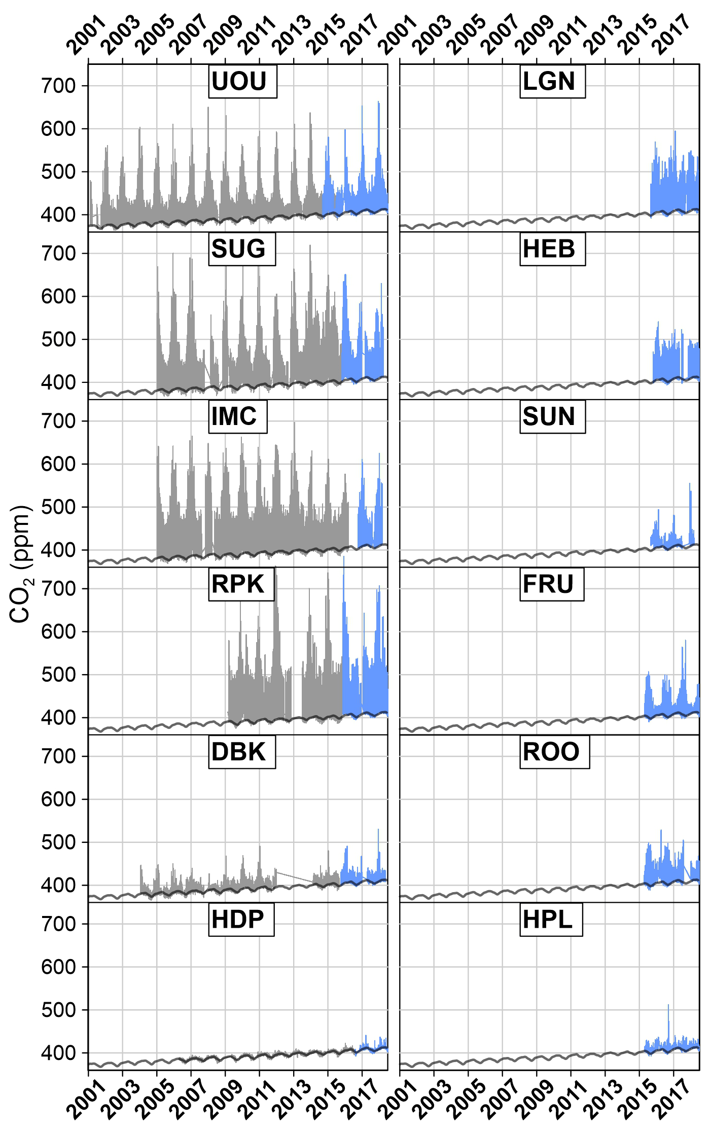
Figure 2Full record time series of CO2 measurements from the UUCON and Uintah Basin GHG. Measurement techniques and uncertainty covered in this paper indicated in blue with historic data represented in gray. The black line represents regional background as described in Mitchell et al. (2018a).
UUCON collects near-surface data used to (a) understand spatial and temporal variability of emissions (Pataki et al., 2003, 2005; Mitchell et al., 2018b; Bares et al., 2018b), (b) evaluate the accumulation of pollutants during complex meteorological conditions (Pataki et al, 2005; Gorski et al., 2015; Baasanbdorj et al., 2017; Bares et al., 2018b; Fiorella et al., 2018), (c) develop and improve atmospheric transport models (Strong et al., 2011; Nehrkorn et al., 2013; Mallia et al., 2015), (d) validate emissions inventory estimates (McKain et al., 2012; Bares et al., 2018b), (e) investigate relationships between urban emissions and air pollution (Baasandorj et al., 2017; Mouteva et al., 2017; Bares et al., 2018b), and (f) inform stakeholders and policymakers (Lin et al., 2018).
Table 1Site characteristics. Historic sites that have been relocated are not listed. Dates are shown in YYYY/MM/DD format.
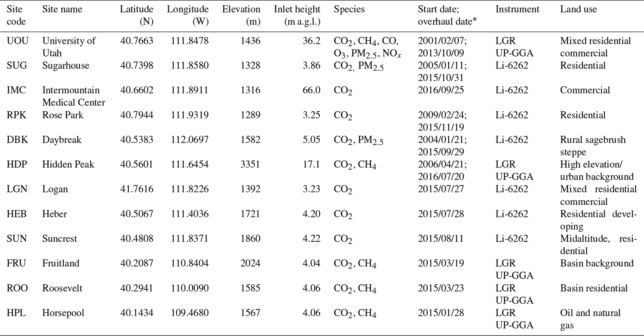
∗ If there is only one date listed then the site is a new installation.
To leverage available infrastructure in urban environments and to increase the signals of intraurban emissions, measurement sites within UUCON are located closer to ground level (Table 1) than tall tower measurement sites. Building-to-neighborhood-scale anthropogenic and biological fluxes contribute more strongly to the UUCON measurements relative to remote-location flask and tall tower observations. Studies comparing tower to near-surface measurements in urban environments have identified an urban canopy effect that leads to elevated nocturnal mole fraction relative to higher above ground level (a.g.l.) measurements (Moriwaki et al., 2006). Thus, the near-surface UUCON data are applicable to research efforts, such as near-field emission studies and smaller-spatial-scale analysis (∼1 km2 footprint, Kort et al., 2013) as well as mapping of spatial and temporal heterogeneities in urban emissions and intracity modeling efforts (Fasoli et al., 2018).
In recent years, cities around the world have launched efforts to establish urban near-surface CO2 monitoring observatories for top-down emission estimates and for modeling validation efforts similar to the UUCON network (Mitchell et al., 2018b). These cities include Los Angeles (Duren and Miller, 2012; Newman et al., 2013; Verhulst et al., 2017), Indianapolis (Turnbull et al., 2015), Paris (Bréon et al., 2015; Staufer et al., 2016), Rome (Gratani and Varone, 2005), Davos, Switzerland (Lauvaux et al., 2013), Portland (Rice and Bostrom, 2011), and Boston (Sargent et al., 2018), among others (Duren and Miller, 2012). In these studies the number of measurement locations utilized is fewer than five, with many using a single measurement location to quantify city-wide CO2 variability, with the notable exceptions of Indianapolis (Turnbull et al., 2015) and Los Angeles (Verhulst et al., 2017). While each of these studies employs somewhat similar measurement techniques, UUCON is unique in its length of record (Mitchell et al., 2018b).
Starting in 2015, the University of Utah deployed a network of high-frequency, high-precision instruments aimed at continuously measuring CO2 and CH4 from areas in eastern Utah where oil and natural gas extraction activities are prevalent (Figs. 2 and 3). This network is known as the Uintah Basin GHG network. These efforts were built on work previously conducted estimating fugitive CH4 emissions (Karion et al., 2013) and the resulting local air quality problems (Edwards et al., 2013, 2014; Koss et al., 2015). The methods developed for the measurements in the Uintah Basin GHG network have also been adopted at two UUCON sites to add CH4 observations to the urban CO2 record.
The aim of this paper is to describe the UUCON and Uintah Basin GHG measurement procedures, site locations, and data structure with sufficient detail to provide documentation for analyses using these datasets, thereby serving as an in-depth method reference. Furthermore, we developed a novel method for exploring and quantifying the measurement uncertainty which was used to analyze the performance of the network over multiple years, to provide insight into appropriate applications of the data, and to explore differences in data collection methods and instrumentation types. This unique method does not require the presence of a target tank within the dataset, allowing for it to be broadly applicable to many trace gas and air quality datasets that are limited to calibration information alone.
Currently, UUCON is comprised of nine sites that are dispersed across northern Utah (Fig. 1, Table 1). Six of the sites are in the Salt Lake Valley (SLV), the most heavily populated area of Utah with over 1 million residents as of this writing and where Salt Lake City, the state capital, is located. The SLV is surrounded by mountains on all sides except for the northwestern part, where it borders the Great Salt Lake (Fig. 1). Sites in the SLV span multiple characteristics and land uses including residential, midaltitude, mixed-use industrial, and rural. Two additional sites are located in the rapidly developing surrounding Heber and Cache valleys, where the towns of Heber City and Logan are located. Both sites in the developing surrounding valleys are located in predominately residential or mixed commercial zones. In addition to the valley-based sites, a nearby high-altitude CO2 monitoring station (HDP), originally started and maintained by the National Center for Atmospheric Research as part of the Regional Atmospheric Continuous CO2 Network in the Rocky Mountains (RACCOON; Stephens et al., 2011), has monitored CO2 levels that serve as a regional background. The HDP site transitioned into the UUCON network in Fall 2016, at which time CH4 observations were added, and continues to be maintained by the University of Utah.
Additionally, the University of Utah maintains a network of three greenhouse gas (GHG) monitoring sites in the Uintah Basin of eastern Utah, where energy extraction is taking place, measuring both CO2 and CH4 (Figs. 1, 2, and 3; Table 1). The measurement techniques used in the Uintah Basin GHG network differ from UUCON in several ways including the use of a different analyzer and will be discussed in detail in Sects. 2.2 and 4. These methods have been adapted at two sites within the UUCON network (HDP and UOU) in an effort to add more GHG measurements (CH4) to the data record.
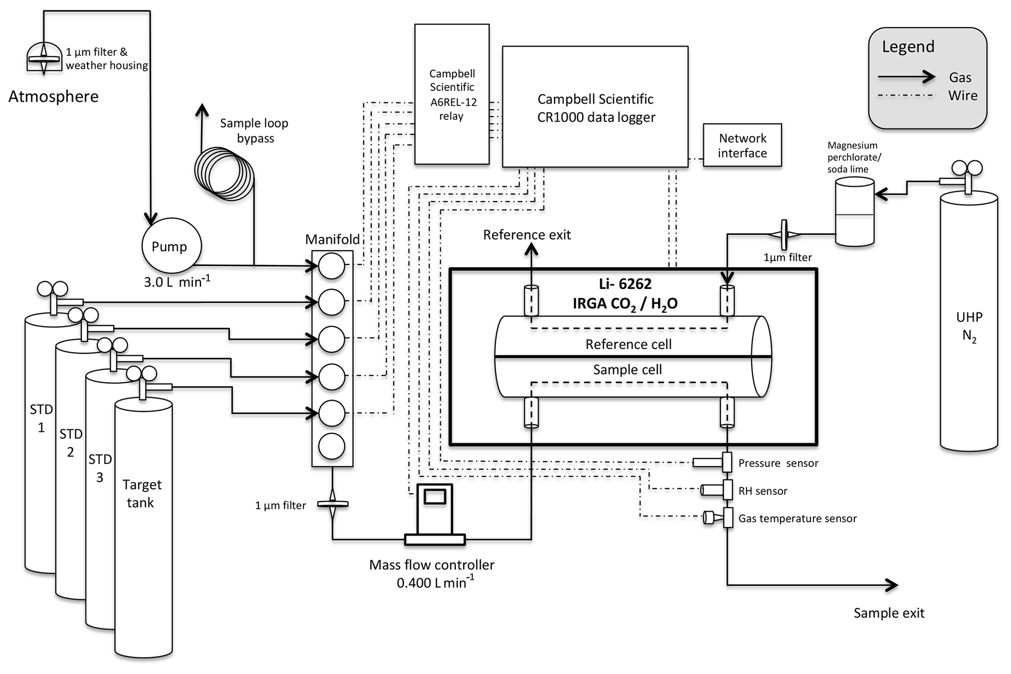
Figure 4Diagram of UUCON measurement design (not to scale). Sites with this design are identified in Fig. 1 with blue triangles. STD: standard tank.
2.1 UUCON instrumentation
Starting in 2001, researchers at the University of Utah deployed Li-6262 (LI-COR Inc., Lincoln, NE) infrared gas analyzers (IRGAs) to measure CO2 mole fractions in the SLV. Previous papers have described various different phases of the initial measurement sites (Pataki et al., 2003, 2005, 2006, 2007) (Fig. 2). This paper will focus on the methods and instrumentation developed in 2014 and implemented across the network by summer of 2016, as well as the methods developed for the Uintah Basin GHG network (Fig. 3). Much of the equipment and materials used during the original phase of the network informed the selection of materials for the 2015 overhaul; however, all components with the exception of the IRGA's were replaced or rebuilt completely, and the methods driving these components are significantly different or improved compared to the original design. Additional components were added to increase the functionality, stability, and the maintenance of measurement sites (Fig. 4).
At each site, sample gas is continuously passed through the sample cell of a Li-6262 to measure CO2 and H2O mole fractions (Fig. 4, Sect. 2.1.1). A small positive pressure is maintained throughout the analyzer and measurement system to make the identification of leaks easier and to reduce the impact on the accuracy of data in the event of a leak. Data are recorded as 10 s integrations of 1 s scans.
The historic method was a noncontinuous method, which collected data on a 5 min interval. Every 5 min a pump would turn on and flow gas for 90 s and then turn off, and the system would then wait 30 s for the IRGA to reach a stable pressure. After the stabilization period, data were recorded by a data logger as a 1 min average of 10 s scans. The system would then sit idle, without flowing gases or recording data until the next sample period.
The decision to change from the historical method to one that continuously flows gas and collects data was in an effort to better capture higher-frequency variations in observed values that could indicate near-field emissions. High-frequency data allow for easier identification of highly localized emissions (e.g., furnace, car) that can affect the signal at a site. Finally, while current atmospheric models are limited in their ability to address near-field emissions effectively, advances in modeling efforts and computational resources make this type of analysis feasible in the near future (Fasoli et al., 2018). Thus the high-frequency collection of UUCON data is in anticipation of future model and analysis needs.
Multiple additional measurements are made to ensure the site's reliable performance, increase measurement accuracy, and to assist in identifying instrumentation problems when they arise (Sect. 2.1.7). All data are downloaded and displayed in real time on a public website (http://air.utah.edu, last access: 22 August 2019) to reduce the time required to identify equipment failure and to provide public outreach. Pressure and water-vapor-broadening corrections, as well as data calibration, are performed post data collection and will be described in depth later (Sect. 3). Two sites in the UUCON network, UOU and HDP (Table 1), host an Ultraportable Greenhouse Gas Analyzer (915-0011, Los Gatos Research, San Jose, CA) on-site. These sites use similar methods to those instrumented with the Li-6262 and will be discussed in depth in Sect. 2.2.
Lastly, the historic measurement design of UUCON included a 5 L mixing buffer, which provided a physical mechanism for smoothing atmospheric observations and reducing instances of large deviations in observations. After moving to a continuous flow design, the buffer has been removed to enable us to measure high-frequency variations. Smoothing can still be achieved at the postprocessing and data analysis stages.
2.1.1 Infrared gas analyzer (IRGA)
A Li-6262 infrared gas analyzer (IRGA) continuously measures CO2 and H2O mole fraction. The IRGA contains two optical measurement cells and quantifies CO2 mole fraction as the difference in absorption between the two cells with a 150 µm bandpass optical filter centered around 4.62 µm. To achieve a mole fraction measurement relative to zero, a CO2-free gas (ultra-high-purity nitrogen) is flowed through the reference cell while the gas of interest in passed through the sample cell (Fig. 4).
2.1.2 Data logger
A Campbell Scientific data logger (CR1000, Campbell Scientific, Logan, UT) acts as both a measurement interface and control apparatus at each site. The data logger records serial data streams from the gas analyzer, as well as analog voltage measurements from the gas analyzer and all additional periphery measurements. Periphery measurements include flow rates, room temperature, sample gas pressure, sample gas temperature, and sample gas relative humidity. Several sites have additional air quality measurements that are recorded by the CR1000 (Table 1) which are not discussed here. The CR1000 is also responsible for driving the calibration periphery that introduces standard gases to the IRGA every 2 h (Sect. 2.1.7).
2.1.3 Pump and sample loop bypass
Atmospheric sample air is pulled from the inlet to the analyzer using a 12 V chemically resistant micro diaphragm gas pump (UNMP850KNDC-B, KNF Neuberger Inc., Trenton, NJ) that provides a reliable flow of 4.2 L min−1. This flow rate is substantially higher than the 0.400 L min−1 sample flow rate selected for use at the analyzer. Thus, the pump is located upstream of the manifold where a sample loop bypass provides an alternative exit for unused sample gas. This loop is comprised of at least 9 m of outer diameter (OD) ( inner diameter) Bev-A-Line tubing to provide sufficient resistance to the gas so, when the manifold is open, gas passes through the mass-flow controller and into the analyzer at the desired rate without losing all of the gas to the sample loop bypass (Fig. 4).
Since the pump is located upstream of the analyzer there is potential for CO2 to absorb onto the material within the pump head and interference with the atmospheric sample. The pumps used in the UUCON network were selected to minimize any potential interference with the sample. The diaphragms are made of a PTFE-coated EPDM rubber which has been shown to have minimal gas-phase absorption. Multiple laboratory and field tests were performed to verify that the location of the pump upstream of the analyzer would not impact the observations. No measurable impacts were identified that provide us with a reasonable level of confidence that any absorption or interference from the pump is negligible.
2.1.4 Relays, manifold, and valves
Switching from sample gas to calibration gases is achieved using a six-position 12 V relay (A6REL-12, Campbell Scientific, Logan, UT), triggered by the data logger at a known interval, connected to a six-port gas manifold (Ev/Et 6-valve, Clippard Instrument Laboratory, Inc., Cincinnati, OH) housing 12 V Clippard relay valves (ET-2-12, Clippard Instrument Laboratory, Inc., Cincinnati, OH). Thus, when the program on the data logger specifies, the CR1000 triggers a relay closing the sample valve and introducing a gas of known CO2 mole fraction. Since the maximum number of gases used at each sampling location is five, the unoccupied position on the relay is often used to power the atmospheric sample pump.
2.1.5 Mass-flow controller
A Smart-Trak 50 mass-flow controller (Sierra Instruments, Monterey, CA) is located between the manifold and analyzer to hold the sample flow consistent at 0.400 SL min−1 (SL stands for standard liters) (Fig. 4). Flow rates are recorded by analog measurement to the CR1000 to ensure a positive pressure remains consistent and to help identify measurement issues remotely.
2.1.6 Calibration materials
Each site houses three whole-air, high-pressure cylinders with known CO2 mole fraction which are directly linked to World Meteorological Organization X2007 CO2 mole fraction scale (Zhao and Tans, 2006), which generally last around 1 year in the field. Every 2 h, the three calibration tanks are introduced to the analyzer in sequence. Each transition of gas begins with a 90 s flush period followed by a 50 s measurement period, or 2 h (minus calibration time) in the case of atmospheric sampling.
The molar fractions of calibration gases are chosen in an effort to span expected atmospheric observations. Values of the three reference materials are chosen to align with the 5th, 50th, and 95th percentile of the previous year's seasonal network-wide observations (Fig. 5). Utilization of previous observations as a reference allows for a guided estimate of expected observations, thereby allowing for a minimization of interpolation without increasing extrapolation significantly, thus limiting extrapolation bias during calibrations.
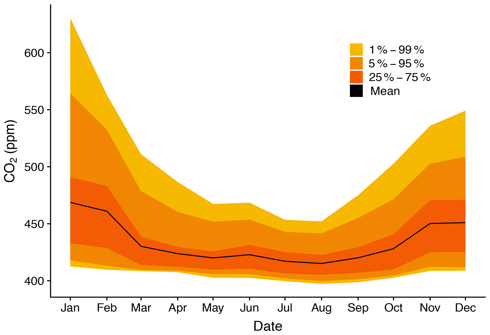
Figure 5Monthly percentiles of atmospheric observations from SUG over one year, 2017. Note that observations in the 95th percentile are greater than 550 ppm CO2, which is well beyond the current WMO calibration scale.
In addition to the standard calibration gases, a long-term target tank is introduced to the analyzer every 25 h. This tank is used to quantify performance of the site as well as determine the accuracy of postprocessed calibrated data. The interval of 25 h was selected to ensure that the calibration occurs at a different time each day in order to remove any consistent diel basis and to prevent the loss of atmospheric observations at a reoccurring time. The target tanks were targeted to be slightly elevated above ambient mole fraction, with the average of 432.02 ppm CO2.
Calibration gases are produced in-house using a custom compressor design. The 29.5 L volume N150 CGA-590 aluminum tanks are filled with city air using a high-pressure oil-free industrial compressor (SA-3 and SA-6, RIX Industries, Benicia, CA). This system is similar to the NOAA ESRL Global Monitoring Division's (GMD) system (http://www.esrl.noaa.gov/gmd/ccl/airstandard.html, last access: 12 May 2019). Water is removed prior to the tanks using a magnesium perchlorate trap to guarantee a dry gas. Tanks are spiked using a ∼5000 ppm dry CO2 tank allowing for a wide range of targeted mole fractions depending on the season and expected range of observed atmospheric observations. This spike tank was filled in the calibration lab by taking an aliquot from a 100 % CO2 gas cylinder and filling it with dried atmospheric air. To produce subambient calibration tanks, tanks are mixed with a diluent made from atmospheric air scrubbed with a soda lime and magnesium perchlorate trap.
Our facility maintains a set of nine standard tanks originally calibrated by the NOAA ESRL's GMD that range from 328 to 800 ppm (during 2000–2004, directly linked to WMO Primary cylinders). Five of the original laboratory primary tanks were remeasured by GMD in 2011–2012 and were found to be lower than the originally measured CO2 mole fraction by 0.10 to 0.51 ppm.
Laboratory primary tanks (which span 350–600 ppm) are propagated from the above tanks into laboratory secondary tanks using a dedicated Li-7000 (LI-COR Biosciences, Lincoln, NE), and these are used in groups of five to calibrate working tertiary tanks used in the field. Secondary tanks are replaced as needed; since measurements began, nine secondary tanks have been used. Secondary calibration tanks are periodically remeasured relative to the WMO-calibrated tanks and are generally within 0.5 ppm of the original measurement. To assign a known mole fraction number to tertiary working calibration tanks, each tank is measured over a minimum of 2 d, with a minimum of three independent measurements per day. In a recent laboratory intercomparison experiment (WMO Round Robin 6), our facilities' results were within 0.1 ppm of established WMO values (https://www.esrl.noaa.gov/gmd/ccgg/wmorr/wmorr_results.php).
The same methods used for developing laboratory primary, secondary, and tertiary CO2 tanks were used for CH4 calibration materials with five original tanks spanning from 1.489 to 9.685 ppm CH4. Two of these tanks are directly tied to the WMO X2004A scale (Dlugokencky et al., 2005). These tanks are propagated into laboratory standards using a dedicated LGR greenhouse gas analyzer (Los Gatos Research, 907-0011, San Jose, CA). The spike tank used to produce elevated CH4 calibration tanks was generated using the same method as the CO2 spike tank but using an aliquot from a 998 ppm CH4 cylinder purchased from Airgas, Inc. (Pennsylvania) and filling it with dried atmospheric air.
As shown in Figs. 2 and 5, wintertime CO2 mole fraction in the SLV can reach over 650 ppm, with the 95th percentile over 550 ppm. As global CO2 mole fractions increase in parallel with increasing populations in the SLV and urban areas of the Wasatch Front (Harbeke et al., 2014), the frequency and amplitude of these highly elevated observations will increase. Currently the WMO X2007 CO2 scale has a maximum mole fraction of 521.419 ppm. Thus, the current WMO scale may be inadequate for urban observations in the SLV, and the announced expansion of the WMO scale to 600 ppm will greatly benefit the urban trace gas community, which needs additional high-quality gas standards with mole fractions more appropriate to urban observations.
2.1.7 Additional measurements
Three additional measurement sensors were added to the downstream side of the IRGA on the sample line to provide additional data for identifying equipment failure and to increase the accuracy of dry mole measurements. A pressure transducer (US331-000005-015PA, Measurement Specialties Inc., Hampton, VA) is located closest to the analyzer to represent pressures in the sample cell of the IRGA. This data stream is used for postprocessing pressure-broadening and water dilution corrections. Uncertainties in the precision and long-term stability of H2O mole fraction measurements performed by the IRGA, due to a lack of frequent calibrations of water vapor, led to the addition of a relative humidity sensor (HM1500LF, Measurement Specialties Inc., Hampton, VA) and a direct immersion thermocouple (211M-T-U-A-2-B-1.5-N, Measurement Specialties Inc., Hampton, VA) for gas relative humidity and temperature measurements preformed immediately after the pressure transducer respectively (Fig. 4). These measurements are utilized to calculate atmospheric H2O ppm, which is used to calculate CO2 dry mole fraction and correct for water vapor broadening (Sect. 3.3).
2.1.8 Network Time Protocol
Intersite comparison and modeling applications require a high degree of confidence in the time stamp represented in data files. To verify the time stamps are consistent between sites and accurate, a network time check is executed every 24 h at 00:00 UTC. If the difference between the network clock and the clock on the data logger is greater than 1000 µs, the data logger clock is reset to match the network clock. All times are recorded in UTC to avoid potential confusion associated with daylight savings. Network time checks and data transfers are established via internet connections at each site either through existing ethernet connections or cellular modems (RV50, Sierra Wireless, Carlsbad, CA).
2.2 Uintah Basin GHG network instrumentation
The Uintah Basin GHG network utilizes the Los Gatos Research Ultraportable Greenhouse Gas Analyzer (907-0011, Los Gatos Research Inc., San Jose, CA), hereafter referred to as “LGR”, at all three sites within the network (Fig. 6). Unlike the UUCON network, in which the measurement system and its peripheries are essentially a custom-engineered solution of an array of different components from multiple manufactures brought together by the researchers running the network, the LGR sites employ systems fully designed by a single manufacturer. The use of an off-the-shelf unit like that deployed in the Uintah Basing GHG network has both advantages and disadvantages. The barrier of entry is much lower and does not require advanced programming abilities. However, the increase in ease of use results in a decrease in the flexibility of operation, and in some cases the measurement precision decreases (Sect. 4).
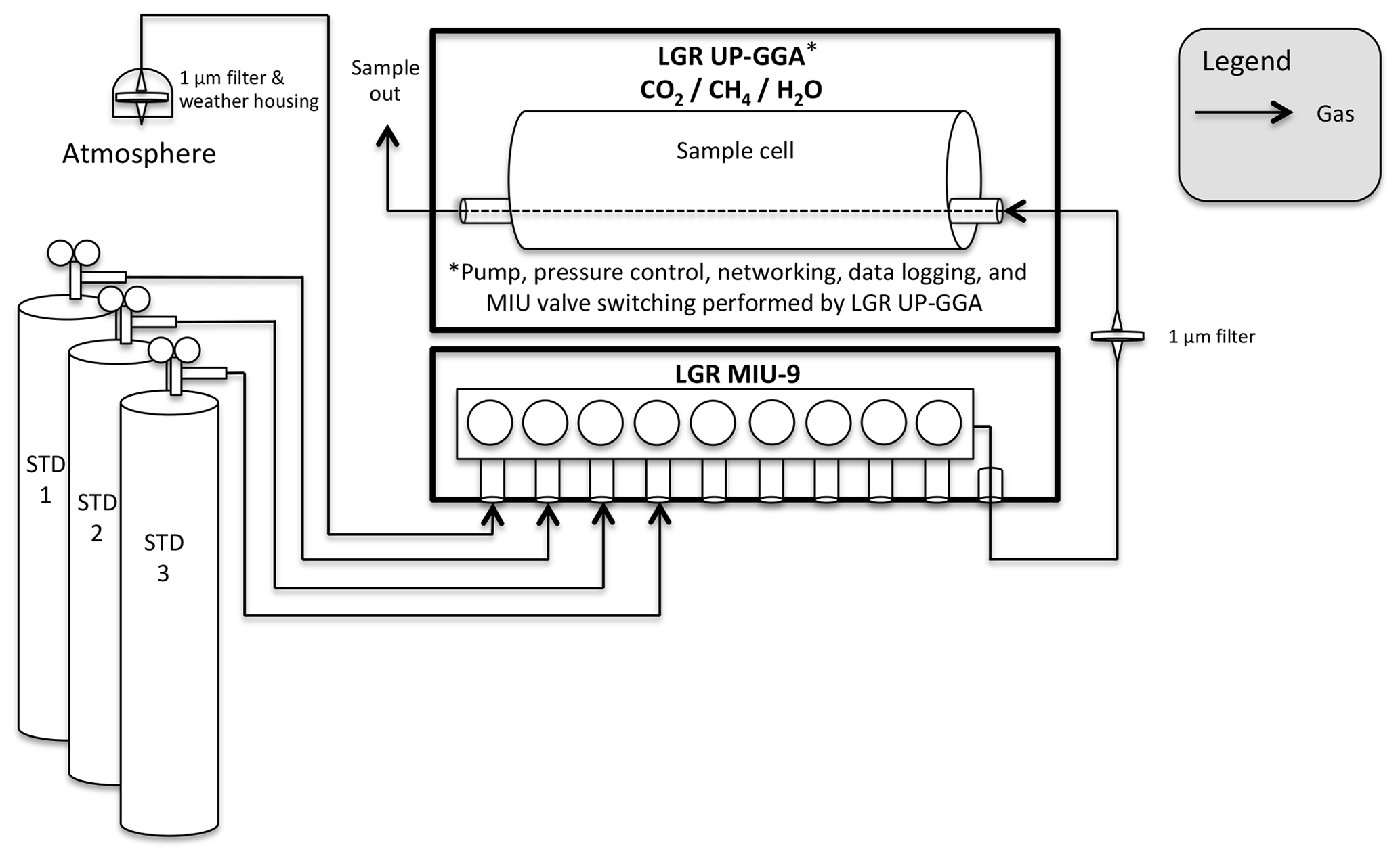
Figure 6Diagram of Uintah Basin greenhouse gas network measurement design. Sites with this design are identified in Fig. 1 with red triangles.
The Uintah Basin GHG network has supported several recent projects including Foster et al. (2017, 2019), in which the data collected from this network were used to estimate and confirm basin-wide CH4 emissions and examine CH4 emissions during wintertime stagnation episodes respectively. In an effort to minimize differences between the two networks, measurement frequency, networking, calibration materials (Sect. 2.1.6), and postprocessing calibration methods (Sect. 3.1) all follow the same protocols described for the UUCON network with the notable exception of the calibration frequency, which is every 3 h as opposed to every 2 h with the Li-6262s.
2.2.1 LGR calibrations
Calibration gases are introduced to the analyzer every 3 h using three whole-air, high-pressure reference gas cylinders with known CO2 and CH4 mole fraction that are directly linked to the WMO X2007 CO2 mole fraction scale (Zhao and Tans, 2006) and the WMO X2004A CH4 mole fraction scale (Dlugokencky et al., 2005) as described in Sect. 2.1.6. Molar fractions of CH4 calibration gases are chosen to align with the 5th, 50th, and 95th percentile of the previous year's observations, while CO2 gases match those described in Sect. 2.1.6. Calibration gases are introduced using an LGR Multiport Input Unit (MIU-9, Los Gatos Research Inc., San Jose, CA). H2O mole fractions are calibrated using a LI-COR Li-610 dew point generator (LI-COR Inc., Lincoln, NE) approximately every 3 months.
2.2.2 LGR H2O and pressure corrections
The LGR analyzer measures mole fraction of H2O, CO2, and CH4, the later two of which are impacted by the presence of water vapor in the sample and the pressure within the cavity of the instrument. Corrections for pressure, water vapor dilution, and spectrum broadening for CH4 and CO2 are made on-site by LGR's software and validated empirically by laboratory testing using calibration gases of know concentrations and the same Li-610 dew point generator described above, which generates a stable dew point at a set temperature (±0.2 ∘C). Independent error estimates of the LGR's H2O correction were produced (Sect. 4, Table 3), resulting in an average uncertainty of 0.017 ppm CO2.
2.2.3 LGR additional considerations
The addition of a target tank, as described in Sect. 2.1.6, would be greatly beneficial for analyzing the long-term performance of each measurement site. However, the current version of the LGR proprietary software that drives the MIU calibration unit lacks flexibility to accommodate a calibration sequence independent of a standard sequence, and thus a target tank was not implemented in the Uintah Basin GHG network design.
For both the UUCON and the Uintah Basin GGA network, raw data are pulled from each site on a 5 min interval to the Center for High Performance Computing at the University of Utah. Data are then run through an automated calibration and quality assurance program described below and made publicly available at https://air.utah.edu.
3.1 Calibrations
Data from UUCON measurement sites with a Li-6262 on-site (Table 1) are calibrated every 2 h using the three reference gases outlined in Sect. 2.1.6, while sites with a LGR are calibrated every 3 h. Since the Li-6262s are near linear through the range of atmospheric observations and calibration gases, each standard of known mole fraction is linearly interpolated between two consecutive calibration periods to represent the drift in the measured standards over time (Fig. 7). Ordinary least squares regression is then applied to the interpolated reference values, and the linear coefficients are used to correct the observations (Fig. 7). The linear slope, intercept, and fit statistics are returned for each observation for diagnostic purposes.
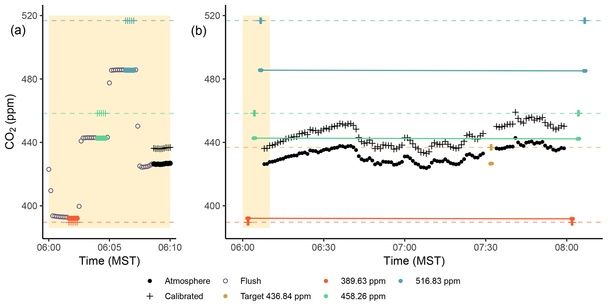
Figure 7Panel (a) shows the sequence and timing of a standard calibration period in both the UUCON and Uintah Basin network. Gray open circles indicate the 90 s flushing period observed between each change in gas. Panel (b) shows a full 2 h sample period with calibrations for the UUCON network with linear interpolations; flush periods have been removed. Orange, green, and blue closed circles indicate calibration standard gases and their known CO2 concentration. The yellow closed circle represents the target tank and its known concentration. Black closed circles indicate precalibration atmospheric observations which have been downsampled to 1 min averages to reduce overplotting. Plus (+) signs in all colors indicate the calibrated measurements for the corresponding measurement.
3.2 Pressure corrections
Changes in ambient atmospheric pressure can impact the measurement of CO2 mole fraction. Pressure effects can be mathematically accounted for or minimized or eliminated by maintaining a constant flow in the optical cavity during calibration and atmospheric sampling periods, as well as calibrating at a high enough frequency that differences in atmospheric pressure between calibration periods are minimal. To account for pressure, the LGRs control the pressure within the cavity and maintain a near-constant 140 Torr. The Li-6262s in the UUCON network do not have mechanisms for controlling the pressure within the cavity and thus implement the latter strategy described above, calibrating frequently and standardizing the flow of gases through the optical cavity.
3.3 Water vapor calculations and corrections
To report dry mole fractions, the presence of water vapor (H2O) must be accounted for. The presence of water vapor impacts measured CO2 mole fraction through both pressure dilution and spectral band broadening. Both of these effects are corrected for during the postprocessing of UUCON data while the LGR sites rely on LGR's internal software. H2O mole fractions are calculated using the relative humidity, pressure, and temperature measurements (Sect. 2.1.7) to first determine saturation vapor pressure utilizing the Clausius–Clapeyron relation with Wexler's equation (Wexler, 1976) below:
where es is the saturation vapor pressure in Pa; T is the temperature in Kelvin; and coefficients g0–g7 are as follows respectively: , , 0.1887643854×10², , , , , and 0.2858487×101.
Vapor pressure (e) is calculated using es from Eq. (1):
The H2O mole fraction is then calculated by taking the ratio of vapor pressure (e) over total atmospheric pressure (P) and converting to parts per million (ppm).
Due to the law of partial pressures, the presence of H2O decreases measured CO2 mole fraction. As the amount of H2O increases, the CO2 mole fraction must decrease for atmospheric pressure to remain unchanged. Using calculated H2O from Eqs. (1), (2), and (3) we correct for the dilution effect of H2O on the measured atmospheric CO2 using the following equation:
where CO2w is the wet sample of atmospheric CO2 and CO2d is the dry air equivalent. Given realistic atmospheric values for the summer in the SLV, 10 000 ppm H2O and 400 ppm CO2, the dilution correction described in Eq. (4) will result in a positive 4.04 ppm CO2 offset (CO2d=404.04 ppm).
The infrared absorption band utilized by the Li-6262s deployed in the UUCON network is broadened by the presence of H2O resulting in a decrease in the measured CO2 mole fraction. To correct for this effect on the measured CO2w described in Eq. (4), we calculated the CO2d in Eq. (5):
where a=6606.6, b=1.4306, and and details regarding function YC can be found in LI-COR technical documentation (App Note #123, 1991).
Using the same values of 10 000 ppm H2O and 400 ppm CO2, the above equation will result in a −0.66 ppm change. Thus the net correction for both pressure broadening (Eq. 4) and dilution effect (Eq. 5) using the same theoretical H2O and CO2 mole fraction results in a 403.3 ppm CO2 dry mole fraction within the UUCON network.
3.4 Data files
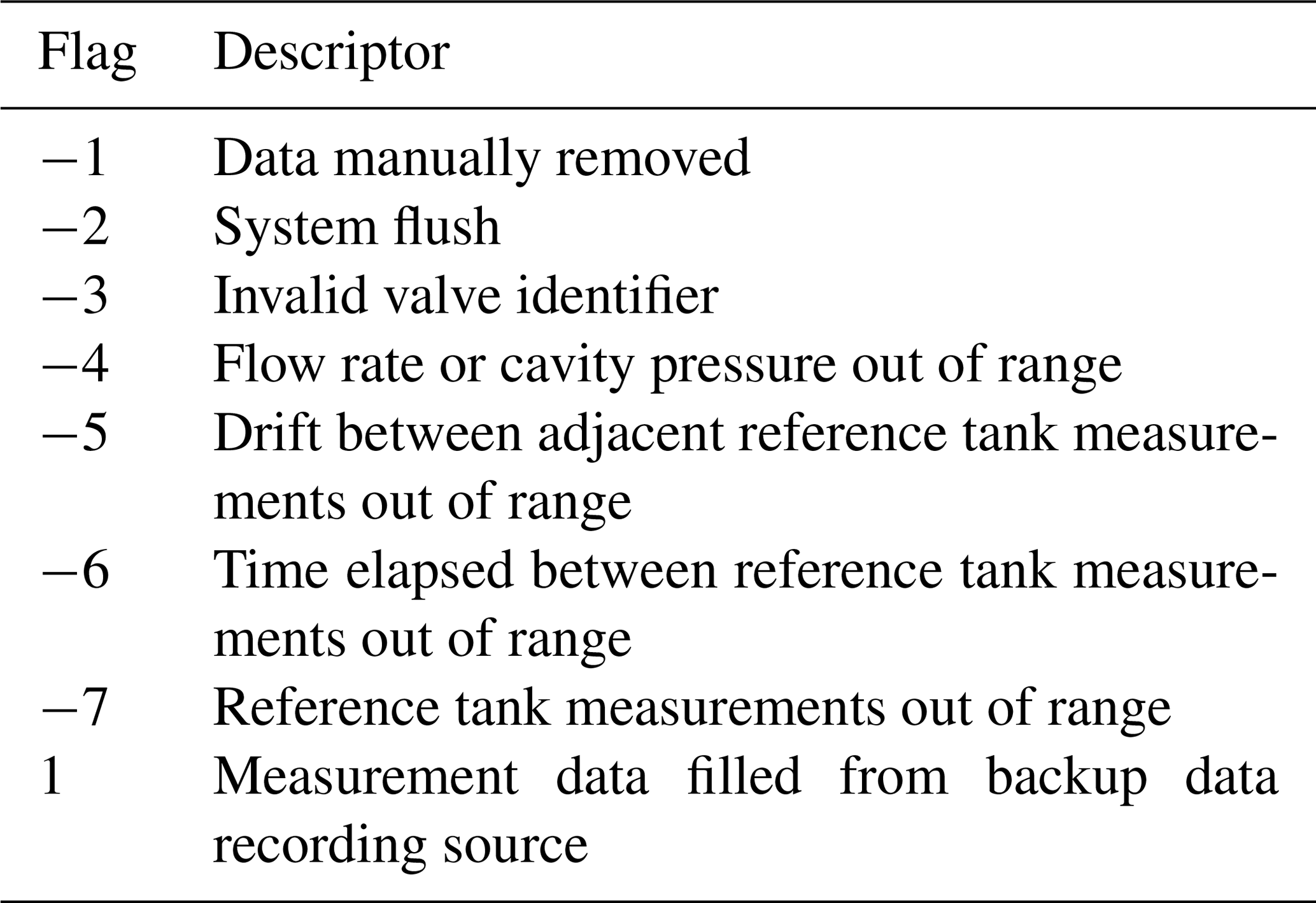
Data are stored at three different levels: raw, QA/QC, and calibrated. Data are stored in monthly files at the native 10 s frequency for all three levels. Raw and QA/QC data files contain an identifier of which gas is currently being measured with atmospheric air identified as −10, flush periods as −99, and standard mole fraction identified as their known mole fraction (i.e., 405.06 ppm).
The lowest level raw data are stored in the same format when pulled from the data logger at the measurement sites. No periods of data are removed from this level and no corrections or calibrations are applied, thus remaining totally unaltered.
The second level of data, QAQC, remains in a similar structure as raw data with a few key exceptions. First, user-specified bad data are removed. A text file containing the periods of bad data is maintained for each site, which is read by automated scripts to remove selected periods. This is a fairly flexible format for removing periods of suspect data that can be easily updated allowing for quick reprocessing of data. Second, automated quality control scripts are run and a column of quality assurance flags is added (Table 2). Lastly, calculation of H2O mole fraction is performed, and CO2 dry mole fraction is calculated as described in Sect. 3.3.
The third and highest level of data, calibrated data, are generated using the QAQC data files. Periods of invalidated records that fail the automated quality control scripts are removed, and calibrations are applied to all remaining data.
3.5 Sample sequence
Since all UUCON measurement sites have only one inlet height, atmospheric sampling is continuous between calibration periods, with no data loss associated with transition periods between sample inlets. During atmospheric sampling, air is drawn from the inlet and passed through the analyzer continuously where it is identified (ID) as the numerical value −10 in the raw and QA/QC data files. Every 2 h, all three of the calibration materials on-site are introduced to the analyzer in sequence, with a 90 s flush period (ID = −99) to allow for equilibration and full changeover of the sample cell, followed by 50 s of measurement time, resulting in a total of 140 s per calibration gas. Figure 7 shows the transition from atmospheric air to a standard gas and the time required to reach equilibration. Every 25 h, a target tank is introduced half way through the hour (i.e., 07:30 MST) using the same sequence described above but treated as an unknown and not utilized in the calibration routine described in Sect. 3.1.
A critical feature of any atmospheric measurement system is an assessment of the system's associated measurement uncertainty. A comprehensive analysis of greenhouse gas measurement uncertainties has been described for the NOAA tall tower network (Andrews et al., 2014) and for the LA Megacities project (Verhulst et al., 2017). Here we have not estimated exhaustively every possible error source. Instead, we have focused on creating a running uncertainty estimate through time that is similar to the approach taken in the INFLUX project (Richardson et al., 2012). Due to the importance of water vapor on the accurate measurement of CO2, especially in a measurement system that does not dry the atmospheric sample like the two described in this paper, we have produced and reported uncertainty estimates for H2O vapor measurements (1) as it impacts CO2 as well as observed analyzer precision (1σUp) in the field (Table 3). We do not report a total, accumulative uncertainty estimate from all possible sources of error combined. Uncertainties beyond those reported here are small compared to the running uncertainty estimate and could be estimated in future work.
Table 3CO2 and CH4 measurement uncertainties with the Gaussian window target tank method (UpTGT), target tank (UTGT), analyzer precision at 1σ (Up), H2O measurement precision 1σ () as expressed in ppm CO2 uncertainty, and data recovery rates from UUCON and Uintah Basin GHG measurement averaged over the entire record since the sites were overhauled. n/a means not applicable.

One method for estimating measurement uncertainties is to use a validation reference gas tank, or “target tank” (UTGT). The target tank is similar to the other calibration gas tanks, but it is not used to calibrate the data and is also sampled at a lower temporal frequency (once every 25 h; Sect. 2.1.7). Since the UUCON network design encompasses a target tank we are able to leverage this method to estimate uncertainty within the network. An example of the target tank measurement is shown in the right panel of Fig. 7, where the target tank was measured at 07:30 MST. The target tank measurements are treated as an unknown and calibrated (Sect. 3.1). The absolute value of the difference between the postcalibrated and known values of the target tank is then calculated. We smoothed the absolute difference time series by convolving it with an 11-point Gaussian window derived according to
where α is 2.5, N is the number of points (11), and n is the sequence between . Prior studies have also used smoothed target tank values to represent measurement uncertainty through time; however, each research group has used a different method. For instance, in the NOAA tall tower network, the 1σ absolute value of the difference between the measured and known target tank mole fractions was calculated across a 3 d processing window (Andrews et al., 2014). In the LA Megacities project, the root mean square error (RMSE) across 11 target tank measurements (measured every 22 h) was used (Verhulst et al., 2017). Finally, in the INFLUX project a running standard deviation of the absolute value of the difference between the measured and known target tank mole fractions over 30 d was used (Richardson et al., 2012). While these approaches differ in their details, each represents an assessment of UTGT through time. Future work could examine how the different target-tank-based uncertainty estimates compare to each other and how they affect atmospheric inversion estimates.
Within the UUCON network, target tanks were incorporated into the experimental design in July 2017 at all of the sites with a Li-6262 analyzer, while sites equipped with a LGR analyzer did not host a target tank, as of this writing. Thus, to estimate the measurement uncertainty at the LGR sites as well as at Li-6262 sites prior to the deployment of the target tanks, an alternative measurement uncertainty method was needed. We produced a method that takes the calibration gas measurements at time t, treats them as pseudo-target tanks, and interpolates the calibration gas measurements between the prior (t−1) and next (t+1) calibration periods to derive a slope and intercept at time t that is then used to calculate the calibrated mole fraction mixing ratios of the pseudo-target tanks and derive an uncertainty estimate. An example of this process is shown in Fig. 8 for the calibration on 27 November 2017 at 18:00 UTC at the IMC site. The calibration gas measurements were interpolated between 16:00 (t−1) and 20:00 (t+1) and used to obtain an interpolated slope and intercept at 18:00 (t) (blue dashed line and triangles in Fig. 8a). The interpolated slope and intercept can be compared to the actual values obtained from the usual calibration procedure (orange circles). The blue dashed line illustrating the interpolation procedure is only shown between 16:00 and 20:00 for clarity, but this process was repeated for each calibration time period. The interpolated slope and intercept were then used to calibrate the pseudo-target-tank measurements at t (blue triangles in Fig. 8b). The RMSE between the calibrated and known values of the three pseudo-target tanks was then calculated (gray circles in Fig. 8d). Since the RMSE can vary substantially between calibration points, we smoothed it by convolving it with an 11-point Gaussian window to yield the pseudo-target-tank uncertainty, or UpTGT (blue squares in Fig. 8d). For this example at 18:00, the interpolated calibration intercept resulted in a relatively large deviation of the calibrated pseudo-target-tank mole fractions from their known values that then resulted in an elevated RMSE. The elevated RMSE from this calibration point then persists for several calibration periods (h) in the smoothed UpTGT.
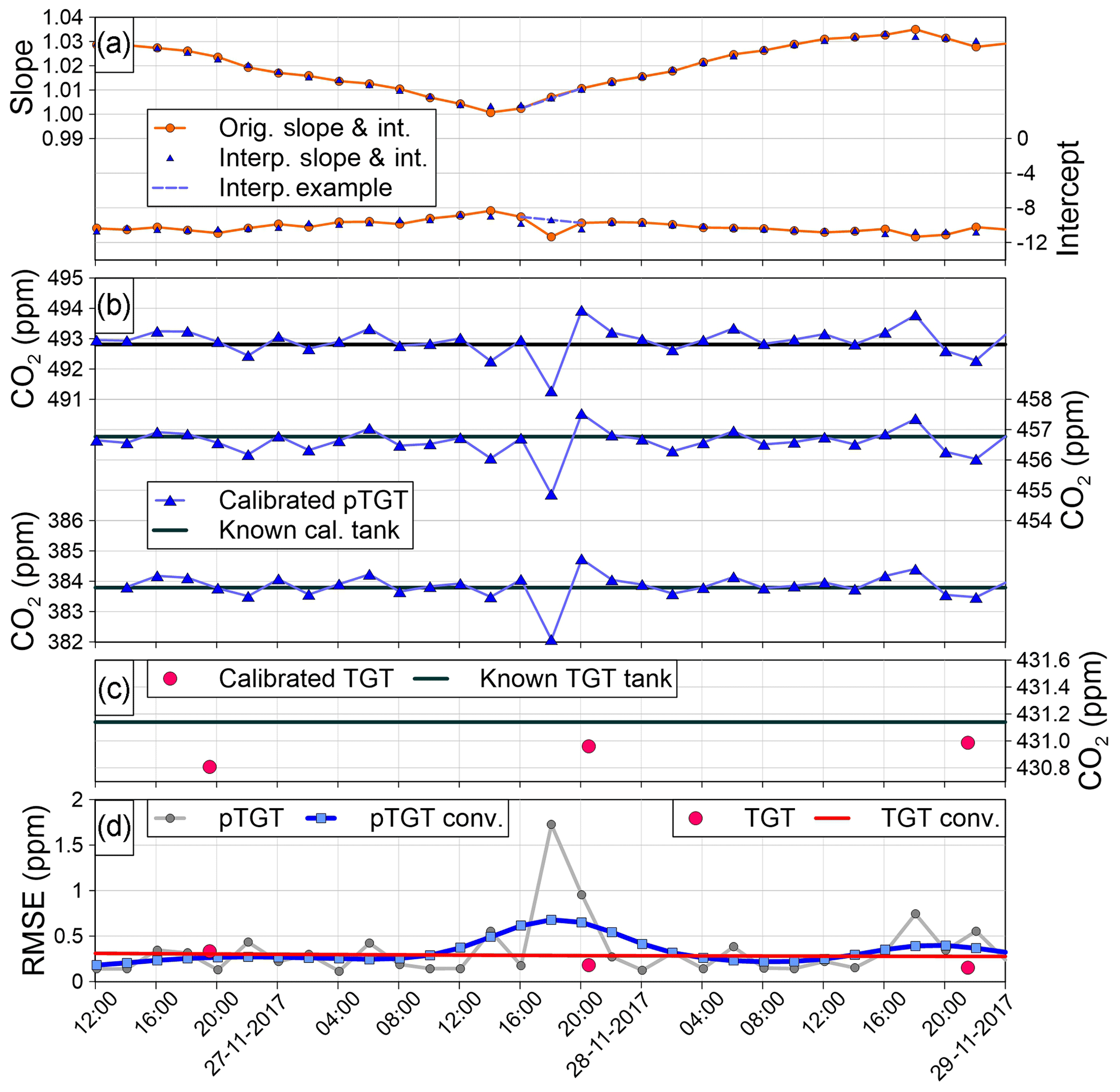
Figure 8Detailed view of the uncertainty analysis at the IMC site. An example of the interpolation procedure is illustrated for the calibration at 18:00 UTC on 27 November 2017 (see the description in the text). The “pTGT conv.” and “TGT conv.” curves in panel (d) are the UpTGT and UTGT uncertainty metrics, respectively.
Once UpTGT was calculated, we compared it to the traditional UTGT over time at the IMC site (Fig. 9). For reference, the yellow shaded region in Fig. 9 is the time period shown in Fig. 8. In July–August 2017 at IMC there was a bias in the postcalibration target tank mole fractions that similarly affected the pseudo-target-tank RMSE values (Fig. 9d). In September 2017 the low-concentration calibration tank was removed from the site for a month and the RMSE values of both metrics improved. Finally, in October 2017 a third calibration tank was reinstalled and there was again a bias in the target tank and pseudo-target tanks. The close fidelity through time between the UpTGT and UTGT metrics provides confidence that UpTGT serves as a robust estimate of measurement uncertainty that is similar to what can be obtained with a traditional target tank. Finally, Fig. 10 shows the entire CO2 UpTGT and UTGT record at all of the sites, while Fig. 11 shows the entire CH4 UpTGT record, with average values reported in Table 3. The UpTGT is reported in the hourly averaged data files as our estimate of measurement uncertainty. It should be noted that since UpTGT is time dependent, gaps in data will result in large uncertainty estimates. As a result we have added a mask, in which any period of data with 8 h or more of missing data is removed from the UpTGT calculation. Additionally, bias in the assigned values of calibration tanks, as well as changes in the distribution of the mole fraction of calibration tanks on-site, can result in stepwise changes in UpTGT as can be seen if Figs. 10 and 11.
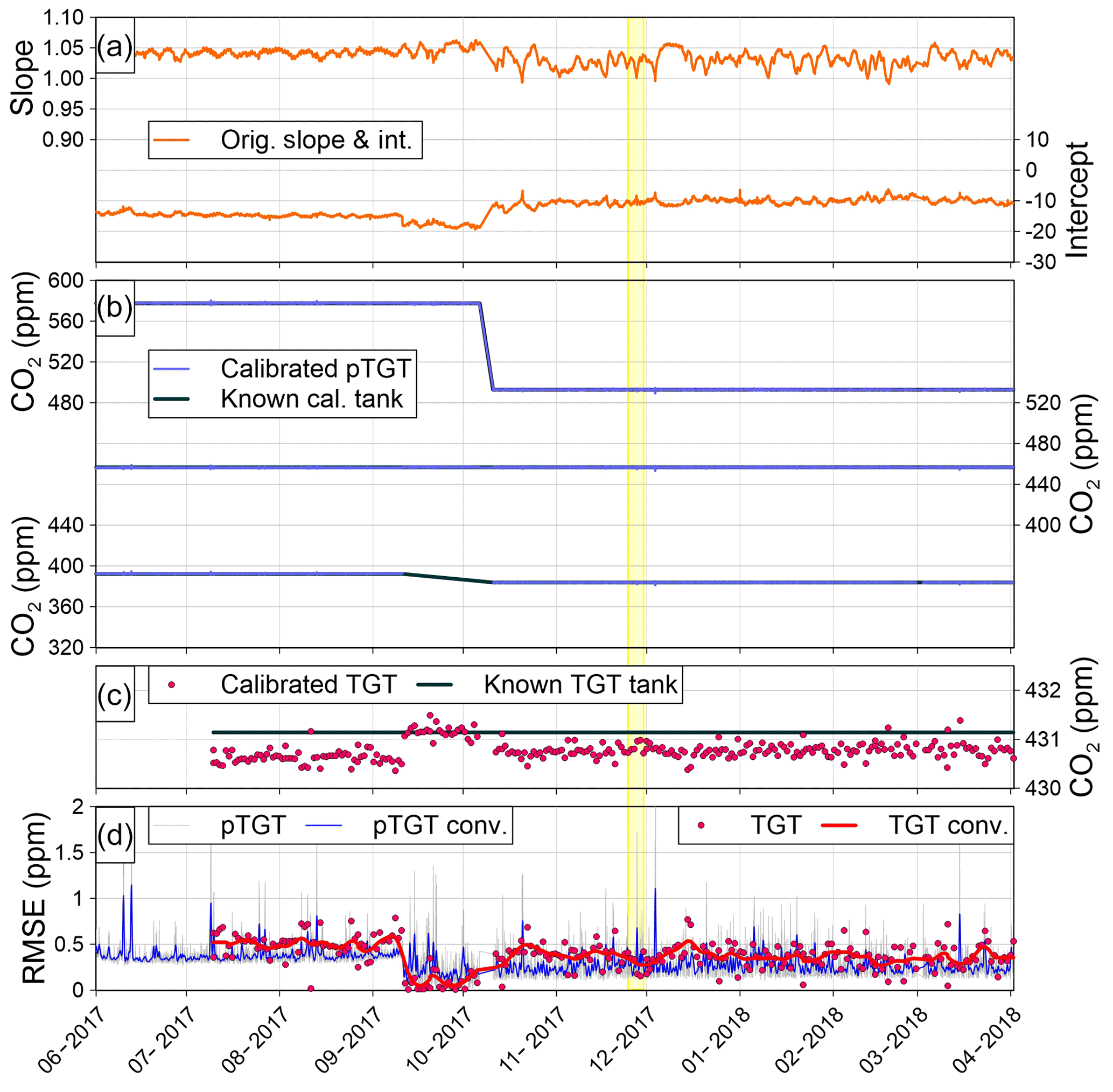
Figure 9Uncertainty analysis at the IMC site for the time period when a target tank was deployed at the site. The “pTGT conv.” and “TGT conv.” curves in panel (d) are the UpTGT and UTGT uncertainty metrics, respectively. The yellow shaded region in Fig. 9 is the time period shown in Fig. 8. See description in text (Sect. 4) for greater detail.
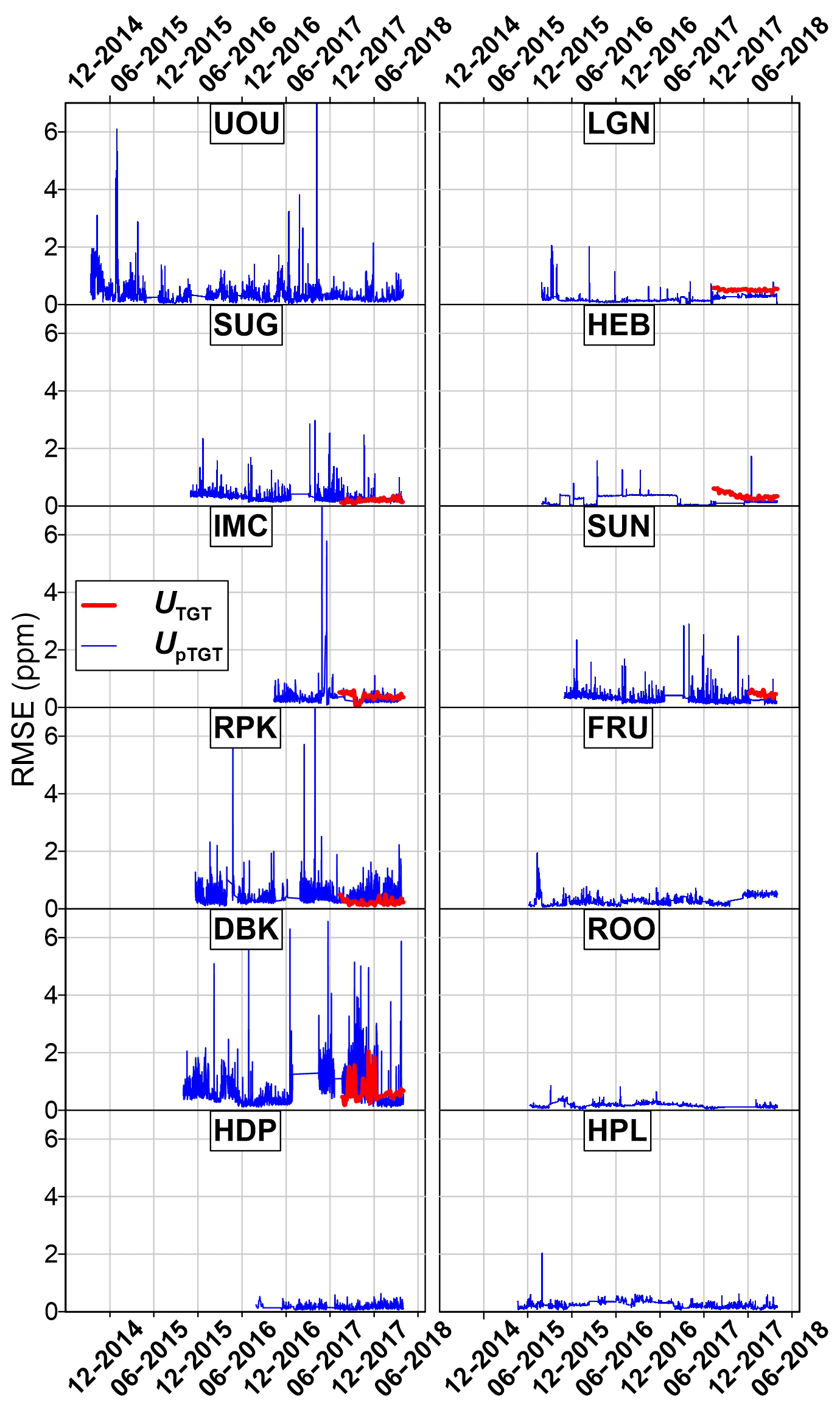
Figure 10Uncertainty analysis for all of the UUCON sites. The UpTGT and UTGT uncertainty metrics are the same as the “pTGT conv.” and “TGT conv” curves in Figs. 8d and 9d, respectively.
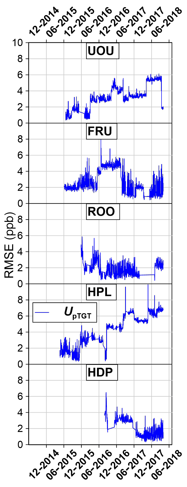
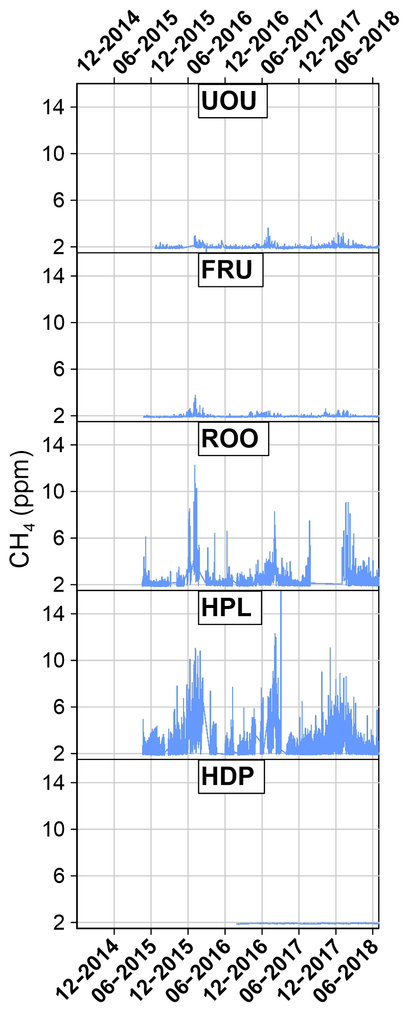
Figure 11CH4 uncertainty analysis. All values reported are the UpTGT uncertainty metrics as shown in Fig. 9d.
The average absolute difference between UpTGT and UTGT at all measurement locations within the UUCON network was 0.03 ppm CO2, suggesting this metric is representative of a more directly measured uncertainty metric like UTGT (Table 3).
Water vapor precision was examined using laboratory tests for the UUCON and the Uintah Basin GHG network designs, which are reported in Table 3 (). Gas from a dry calibration tank of know CO2 mole fraction was passed through a Li-610 dew point generator at a set dew point temperature. H2O measurements were collected by both systems in parallel over a period of 1.5 h. We calculated the Allan variance to represent the precision of the H2O measurements regardless of drift over time or other systematic errors. This precision statistic was used to construct a normal distribution of H2O centered on the mean measured H2O mole fraction at each site, which is used to estimate the uncertainties in dry-air-equivalent estimates for CO2 due to H2O repeatability error using methods discussed in Sect. 3.3. The 1σ uncertainty of the H2O precision results in a mean 0.019 ppm CO2 error () for the UUCON network and 0.017 ppm CO2 for the Uintah Basin GHG network design. These uncertainties represent a lower bound for error in CO2, resulting in H2O measurements as they do not account for errors in H2O measurement accuracy, which can be addressed during the QAQC of data.
A unique aspect of the UUCON and Uintah Basin networks is the use of two different instruments to measure CO2. This allows for the ability to directly compare instrument performance during extended field operations. Table 3 shows the uncertainty metrics described in Sect. 4 and in Figs. 8, 9, 10, and 11. Additionally, the precision of the instruments (Up) at each site is reported as an average value of the standard deviation (1σ) of the calibrated values for each individual calibration gas introduced to the analyzer since the overhaul of the site, the standard deviation (1σ) of H2O measurements expressed in terms of uncertainty added to CO2 ppm as determined by lab tests, and the data recovery rates for each site. Site to site variability in UpTGT ranges from 0.18 to 0.69 ppm CO2 within the UUCON network, with the highest observed uncertainty at sites with more limited environmental controls and a mean value of 0.38 ppm across the entire network. Sites equipped with a LGR ranged from 0.17 to 0.36 CO2 ppm (1.8 to 4.2 ppb CH4), with a mean across all sites of 0.25 ppm CO2 (2.8 ppb CH4). Uncertainty in CO2 ppm resulting from the measurement of H2O () is minimal between sites (0.017 to 0.020 ppm CO2) and has a minimal impact on CO2 uncertainties (Table 3).
Our reported average CH4 UpTGT uncertainty value of 2.8 ppb is notably higher than those reported by other groups quantifying measurement uncertainty, including Verhulst et al. (2017), which reported a value of 0.2126 ppb uncertainty as estimated using the postcalibrated target tank residuals integrated over 10 d of observations, as well as a total CH4 uncertainty (Uair) of 0.7224 ppb from measurements using a Picarro G2301 (Picarro Inc., Santa Clara, CA). Our higher reported values are likely the result of both the use of a different analyzer than a Picarro and the fact that our uncertainty estimates are based on an interpolation between nonsequential calibration periods and not a directly measured target tank.
It is notable that in all but one instance the precision (Up) of the Li-6262's CO2 is twice as precise compared to the LGR's (Table 3), and the one instance is at DBK, which experiences larger temperature ranges, despite the Li-6262s being ∼20 years older than the LGRs. Additionally, the uncertainty and data recovery rates between the two instrument types are highly comparable.
The highly similar CO2 metrics observed between the two instrumentation types suggest that the most significant advantage of the more modern direct absorption LGRs is the addition of a second gas species measured, methane (CH4) in this instance, especially at sites with well-regulated climate controls.
All data described in this paper are archived with the National Oceanic and Atmospheric Administration's (NOAA) National Centers for Environmental Information (NCEI) and can be found at https://doi.org/10.7289/V50R9MN2 (Mitchell et al., 2018c) and https://doi.org/10.25921/8vaj-bk51 (Bares et al., 2018a). All data used in this analysis are available upon request from the corresponding author or can be downloaded at the U-ATAQ's data repository at https://air.utah.edu/data/ (last access: 22 August 2019).
As the global effort to reduce greenhouse gas emissions transitions from commitment to policy measures, greenhouse gas measurement networks provide a means for evaluating progress. The UUCON network is an example of an urban CO2 network well suited for this application due to its long-term duration, precision, and spatial distribution (Mitchell et al., 2018b). With high data recovery rates and low average measurement uncertainty (UpTGT) of 0.38 ppm CO2, the network produces data suitable for a range of scientific and, potentially, policy applications. Additionally, there is increasing interest in performing cross-urban comparisons between different urban environments. Given the reported measurement uncertainties, the frequency of calibrations, and the tractability to international working scales, these data are well situated for this application.
The overhaul of instrumentation and design documented in this paper has resulted in a robust network of reliable data, with additional measurements to remotely identify when problems arise as well as increase the precision of the data. The standardization of materials and measurement protocols at all locations has significantly lowered the barrier of entry for maintenance of the sites.
The addition of target tanks at multiple sites in 2017 allows for the calculation of continuous uncertainty metrics. From those metrics, an interpolation method was developed allowing for uncertainty estimates of sites and networks where a target tank is not available. This novel method for estimating uncertainty provides useful insight into the quality of data produced at individual sites and is broadly applicable to any atmospheric trace gas or air quality dataset that contains calibration information.
The use of the interpolated uncertainty metric, as well as the calculation of the standard deviation of calibration measurements in the field, identified limited differences between the two measurement techniques used in the UUCON and Uintah Basin GHG networks.
Targeted reductions in the emissions of other greenhouse gases, primarily CH4, will require similarly distributed measurement networks for validating reduction progress and tracking emissions, both in urban areas and regions of oil and natural gas extraction. With 3 years of continuous operation to date and relatively low measurement uncertainty (2.8 ppb CH4), the Uintah Basin GHG network serves as a good example of a greenhouse gas network with simultaneous measurements of CH4 and CO2. With comparable precision and reliability to those reported in UUCON, but with the added benefit of two measurement species, the measurement techniques deployed in the Uintah Basin GHG network have been expanded into a few urban locations within the UUCON network.
RB and BF were responsible for the design and implementation of measurement sites. BF developed the real-time visualizations and postprocessing protocols. LM developed the uncertainty metrics and wrote the corresponding sections of the paper. DRB provided critical feedback during the design phase of the network and provided significant portions of the manuscript describing the creation of calibration materials. DRB and MG produced the calibration materials used in the network. DC provided regular maintenance of the network and produced the long-term standard protocols for the UUCON network. BE provided help on the water vapor calculations and corrections. JE and JCL each served as PIs during the development, maintenance, and operation of the network, providing insight and oversight throughout the process. RB prepared the manuscript with contributions from all coauthors.
The authors declare that they have no conflict of interest.
This research was supported by the National Oceanic and Atmospheric Administration (NOAA) grant NA140AR4310178 and NA140AR4310138. The authors would like to thank Britton Stephens and the National Center for Atmospheric Research for establishing the HDP site, Seth Lyman and Utah State University Vernal for their continued support of the Uintah Basin GHG network, and the Stable Isotope Ratio Facility for Environmental Research (SIRFER) at the University of Utah for their commitment to UUCON. We would also like to thank the following hosting institutions: Draper City and the Salt Lake County Unified Fire Authority, Rio Tinto Kennecott, Snowbird Ski Resort, the Salt Lake Center of Science Education, Intermountain Health Center, Utah State University Logan, Utah State University Vernal, Wasatch County Health Department, and the Utah Division of Air Quality.
This research has been supported by the National Oceanic and Atmospheric Administration (grant nos. NA140AR4310178 and NA140AR4310138).
This paper was edited by David Carlson and reviewed by two anonymous referees.
Andrews, A. E., Kofler, J. D., Trudeau, M. E., Williams, J. C., Neff, D. H., Masarie, K. A., Chao, D. Y., Kitzis, D. R., Novelli, P. C., Zhao, C. L., Dlugokencky, E. J., Lang, P. M., Crotwell, M. J., Fischer, M. L., Parker, M. J., Lee, J. T., Baumann, D. D., Desai, A. R., Stanier, C. O., De Wekker, S. F. J., Wolfe, D. E., Munger, J. W., and Tans, P. P.: CO2, CO, and CH4 measurements from tall towers in the NOAA Earth System Research Laboratory's Global Greenhouse Gas Reference Network: instrumentation, uncertainty analysis, and recommendations for future high-accuracy greenhouse gas monitoring efforts, Atmos. Meas. Tech., 7, 647–687, https://doi.org/10.5194/amt-7-647-2014, 2014.
App Note #123: Implementing Zero and Span Adjustments, and the Band Broadening Correction On Measured Data, 3576, 1–6, available at: https://www.licor.com/documents/6yqgna9zt7y6avvg2azs (last access: 15 August 2018), 1991.
Baasandorj, M., Hoch, S. W., Bares, R., Lin, J. C., Brown, S. S., Millet, D. B., Martin, R., Kelly, K., Zarzana, K. J., Whiteman, C. D., Dube, W. P., Tonnesen, G., Jaramillo, I. C., and Sohl, J.: Coupling between Chemical and Meteorological Processes under Persistent Cold-Air Pool Conditions: Evolution of Wintertime PM2.5 Pollution Events and N2O5 Observations in Utah's Salt Lake Valley, Environ. Sci. Technol., 51, 5941–5950, https://doi.org/10.1021/acs.est.6b06603, 2017.
Bakwin, P. S., Tans, P. P., Hurst, D. F., and Zhao, C.: Measurements of carbon dioxide on very tall towers?: results of the NOAA/CMDL program, Tellus, 50, 401–415, https://doi.org/10.1034/j.1600-0889.1998.t01-4-00001.x, 1998.
Bares, R., Lin, J. C., Fasoli, B., Mitchell, L. E., Bowling, D. R., Garcia, M., Catharine, D., and Ehleringer, J. R.: Atmospheric measurements of carbon dioxide (CO2) and methane (CH4) from the state of Utah from 2014-09-10 to 2018-04-01 (NCEI Accession 0183632). Version 1.1. NOAA National Centers for Environmental Information, Dataset, https://doi.org/10.25921/8vaj-bk51, 2018a.
Bares, R., Lin, J. C., Hoch, S. W., Baasandorj, M., Mendoza, D. L., Fasoli, B., Mitchell, L., Catharine, D., and Stephens, B. B.: The Wintertime Covariation of CO2 and Criteria Pollutants in an Urban Valley of the Western United States, J. Geophys. Res.-Atmos., 123, 2684–2703, https://doi.org/10.1002/2017JD027917, 2018b.
Bréon, F. M., Broquet, G., Puygrenier, V., Chevallier, F., Xueref-Remy, I., Ramonet, M., Dieudonné, E., Lopez, M., Schmidt, M., Perrussel, O., and Ciais, P.: An attempt at estimating Paris area CO2 emissions from atmospheric concentration measurements, Atmos. Chem. Phys., 15, 1707–1724, https://doi.org/10.5194/acp-15-1707-2015, 2015.
Dlugokencky, E. J., Myers, R. C., Lang, P. M., Masarie, K. A., Crotwell, A. M., Thoning, K. W., Hall, B. D., Elkins, J. W., and Steele, L. P.: Conversion of NOAA atmospheric dry air CH4 mole fractions to a gravimetrically prepared standard scale, J. Geophys. Res.-Atmos., 110, 1–8, https://doi.org/10.1029/2005JD006035, 2005.
Duren, R. M. and Miller, C. E.: Measuring the carbon emissions of megacities, Nat. Clim. Change, 2, 560–562, https://doi.org/10.1038/nclimate1629, 2012.
Edwards, P. M., Young, C. J., Aikin, K., deGouw, J., Dubé, W. P., Geiger, F., Gilman, J., Helmig, D., Holloway, J. S., Kercher, J., Lerner, B., Martin, R., McLaren, R., Parrish, D. D., Peischl, J., Roberts, J. M., Ryerson, T. B., Thornton, J., Warneke, C., Williams, E. J., and Brown, S. S.: Ozone photochemistry in an oil and natural gas extraction region during winter: simulations of a snow-free season in the Uintah Basin, Utah, Atmos. Chem. Phys., 13, 8955–8971, https://doi.org/10.5194/acp-13-8955-2013, 2013.
Edwards, P. M., Brown, S. S., Roberts, J. M., Ahmadov, R., Banta, R. M., DeGouw, J. A., Dubé, W. P., Field, R. A., Flynn, J. H., Gilman, J. B., Graus, M., Helmig, D., Koss, A., Langford, A. O., Lefer, B. L., Lerner, B. M., Li, R., Li, S. M., McKeen, S. A., Murphy, S. M., Parrish, D. D., Senff, C. J., Soltis, J., Stutz, J., Sweeney, C., Thompson, C. R., Trainer, M. K., Tsai, C., Veres, P. R., Washenfelder, R. A., Warneke, C., Wild, R. J., Young, C. J., Yuan, B., and Zamora, R.: High winter ozone pollution from carbonyl photolysis in an oil and gas basin, Nature, 514, 351–354, https://doi.org/10.1038/nature13767, 2014.
EIA: State Carbon Dioxide Emissions Data, Tech. rep., United States Energy Information Administration, available at: https://www.eia.gov/state/seds/?sid=UT (last access: June 2018), 2015.
Fasoli, B., Lin, J. C., Bowling, D. R., Mitchell, L., and Mendoza, D.: Simulating atmospheric tracer concentrations for spatially distributed receptors: updates to the Stochastic Time-Inverted Lagrangian Transport model's R interface (STILT-R version 2), Geosci. Model Dev., 11, 2813–2824, https://doi.org/10.5194/gmd-11-2813-2018, 2018.
Fiorella, R. P., Bares, R., Lin, J. C., Ehleringer, J. R., and Bowen, G. J.: Detection and variability of combustion-derived vapor in an urban basin, Atmos. Chem. Phys., 18, 8529–8547, https://doi.org/10.5194/acp-18-8529-2018, 2018.
Foster, C. S., Crosman, E. T., Holland, L., Mallia, D. V., Fasoli, B., Bares, R., Horel, J., and Lin, J. C.: Confirmation of elevated methane emissions in Utah's Uintah Basin with ground-based observations and a high-resolution transport model, J. Geophys. Res.-Atmos., 122, 1–19, https://doi.org/10.1002/2017JD027480, 2017.
Foster, C. S., Crosman, E. T., Horel, J. D., Lyman, S., Fasoli, B., Bares, R., and Lin, J. C.: Quantifying methane emissions in the Uintah Basin during wintertime stagnation episodes, Elementa Science of the Anthropocene, 7, 1–24, https://doi.org/10.1525/elementa.362, 2019.
Gorski, G., Strong, C., Good, S. P., Bares, R., Ehleringer, J. R., and Bowen, G. J.: Vapor hydrogen and oxygen isotopes reflect water of combustion in the urban atmosphere, P. Natl. Acad. Sci. USA, 112, 3247–3252, https://doi.org/10.1073/pnas.1424728112, 2015.
Gratani, L. and Varone, L.: Daily and seasonal variation of CO in the city of Rome in relationship with the traffic volume, Atmos. Environ., 39, 2619–2624, https://doi.org/10.1016/j.atmosenv.2005.01.013, 2005.
Harbeke, D. T., Garbett, B., Chairman, V., Matsumori, D., Kroes, S. J. H., and City, S. L.: A Snapshot of 2050, Research Report number 702, Utah Foundation Magazine, 1–16, 2014.
Hutyra, L. R., Duren, R., Gurney, K. R., Grimm, N., Kort, E. A., Larson, E., and Shrestha, G.: Urbanization and the carbon cycle: Current capabilities and research outlook from the natural sciences perspective, Earth's Future, 2, 473–495, https://doi.org/10.1002/2014EF000255, 2014.
IEA: Energy and Climate Change, World Energy Outlook Special Report, 1–200, https://doi.org/10.1038/479267b, 2015.
Karion, A., Sweeney, C., Pétron, G., Frost, G., Michael Hardesty, R., Kofler, J., Miller, B. R., Newberger, T., Wolter, S., Banta, R., Brewer, A., Dlugokencky, E., Lang, P., Montzka, S. A., Schnell, R., Tans, P., Trainer, M., Zamora, R., and Conley, S.: Methane emissions estimate from airborne measurements over a western United States natural gas field, Geophys. Res. Lett., 40, 4393–4397, https://doi.org/10.1002/grl.50811, 2013.
Kort, E. A., Angevine, W. M., Duren, R., and Miller, C. E.: Surface observations for monitoring urban fossil fuel CO2 emissions: Minimum site location requirements for the Los Angeles megacity, J. Geophys. Res.-Atmos., 118, 1–8, https://doi.org/10.1002/jgrd.50135, 2013.
Koss, A. R., de Gouw, J., Warneke, C., Gilman, J. B., Lerner, B. M., Graus, M., Yuan, B., Edwards, P., Brown, S. S., Wild, R., Roberts, J. M., Bates, T. S., and Quinn, P. K.: Photochemical aging of volatile organic compounds associated with oil and natural gas extraction in the Uintah Basin, UT, during a wintertime ozone formation event, Atmos. Chem. Phys., 15, 5727–5741, https://doi.org/10.5194/acp-15-5727-2015, 2015.
Lauvaux, T., Miles, N. L., Richardson, S. J., Deng, A., Stauffer, D. R., Davis, K. J., Jacobson, G., Rella, C., Calonder, G. P., and Decola, P. L.: Urban emissions of CO2 from Davos, Switzerland: The first real-time monitoring system using an atmospheric inversion technique, J. Appl. Meteorol. Clim., 52, 2654–2668, https://doi.org/10.1175/JAMC-D-13-038.1, 2013.
Lin, J. C., Mitchell, L., Crosman, E., Mendoza, D., Buchert, M., Bares, R., Fasoli, B., Bowling, D. R., Pataki, D., Catharine, D., Strong, C., Gurney, K., Patarasuk, R., Baasandorj, M., Jacques, A., Hoch, S., Horel, J., and Ehleringer, J.: CO2 and carbon emissions from cities: linkages to air quality, socioeconomic activity and stakeholders in the Salt Lake City urban area, B. Am. Meteorol. Soc., 99, 2325–2339, https://doi.org/10.1175/BAMS-D-17-0037.1, 2018.
Mallia, D. V., Lin, J. C., Urbanski, S., Ehleringer, J., and Nehrkorn, T.: Impacts of
upwind wildfire emissions on CO, CO2, and PM2.5 concentrations in Salt
Lake City, Utah, J. Geophys. Res.-Atmos., 120, 147–166,
doi10.1002/2017JC013052, 2015.
McKain, K., Wofsy, S. C., Nehrkorn, T., Eluszkiewicz, J., Ehleringer, J. R., and Stephens, B. B.: Assessment of ground-based atmospheric observations for verification of greenhouse gas emissions from an urban region, P. Natl. Acad. Sci. USA, 109, 8423–8428, https://doi.org/10.1073/pnas.1116645109, 2012.
Mitchell, L. E., Crosman, E. T., Jacques, A. A., Fasoli, B., Leclair-Marzolf, L., Horel, J., Bowling, D. R., Ehleringer, J. R., and Lin, J. C.: Monitoring of greenhouse gases and pollutants across an urban area using a light-rail public transit platform, Atmos. Environ., 187, 9–23, https://doi.org/10.1016/j.atmosenv.2018.05.044, 2018a.
Mitchell, L. E., Lin, J. C., Bowling, D. R., Pataki, D. E., Strong, C., Schauer, A. J., Bares, R., Bush, S. E., Stephens, B. B., Mendoza, D., Mallia, D., Holland, L., Gurney, K. R., and Ehleringer, J. R.: Long-term urban carbon dioxide observations reveal spatial and temporal dynamics related to urban characteristics and growth, P. Natl. Acad. Sci. USA, 115, 2912–2917, https://doi.org/10.1073/pnas.1702393115, 2018b.
Mitchell, L. E., Lin, J. C., Bowling, D. R., Pataki, D. E., Strong, C., Schauer, A. J., Bares, R., Bush, S. E., Stephens, B. B., Mendoza, D., Mallia, D., Holland, L., Gurney, K. R., and Ehleringer, J. R.: Carbon Dioxide (CO2) mole fraction, CO2 flux, and others collected from Salt Lake City CO2 measurement network in Western U.S. from 2001-02-07 to 2015-10-23 (NCEI Accession 0170450). Version 1.1. NOAA National Centers for Environmental Information. Dataset. https://doi.org/10.7289/V50R9MN2, 2018c.
Moriwaki, R., Kanda, M., and Nitta, H.: Carbon dioxide build-up within a suburban canopy layer in winter night, Atmos. Environ., 40, 1394–1407, https://doi.org/10.1016/j.atmosenv.2005.10.059, 2006.
Mouteva, G. O., Randerson, J. T., Fahrni, S. M., Bush, S. E., Ehleringer, J. R., Xu, X., Santos, G. M., Kuprov, R., Schichtel, B. A., and Czimczik, C. I.: Using radiocarbon to constrain black and organic carbon aerosol sources in Salt Lake City, J. Geophys. Res.-Atmos., 122, 9843–9857, https://doi.org/10.1002/2017JD026519, 2017.
Nehrkorn, T., Henderson, J., Leidner, M., Mountain, M., Eluszkiewicz, J., McKain, K., and Wofsy, S.: WRF simulations of the urban circulation in the salt lake city area for CO2 modeling, J. Appl. Meteorol. Clim., 52, 323–340, https://doi.org/10.1175/JAMC-D-12-061.1, 2013.
Newman, S., Jeong, S., Fischer, M. L., Xu, X., Haman, C. L., Lefer, B., Alvarez, S., Rappenglueck, B., Kort, E. A., Andrews, A. E., Peischl, J., Gurney, K. R., Miller, C. E., and Yung, Y. L.: Diurnal tracking of anthropogenic CO2 emissions in the Los Angeles basin megacity during spring 2010, Atmos. Chem. Phys., 13, 4359–4372, https://doi.org/10.5194/acp-13-4359-2013, 2013.
Pataki, D. E., Bowling, D. R., and Ehleringer, J. R.: Seasonal cycle of carbon dioxide and its isotopic composition in an urban atmosphere: Anthropogenic and biogenic effects, J. Geophys. Res., 108, 4735, https://doi.org/10.1029/2003JD003865, 2003.
Pataki, D. E., Tyler, B. J., Peterson, R. E., Nair, A. P., Steenburgh, W. J., and Pardyjak, E. R.: Can carbon dioxide be used as a tracer of urban atmospheric transport?, J. Geophys. Res.-Atmos., 110, 1–8, https://doi.org/10.1029/2004JD005723, 2005.
Pataki, D. E., Bowling, D. R., Ehleringer, J. R., and Zobitz, J. M.: High resolution atmospheric monitoring of urban carbon dioxide sources, Geophys. Res. Lett., 33, 1–5, https://doi.org/10.1029/2005GL024822, 2006.
Pataki, D. E., Xu, T., Luo, Y. Q., and Ehleringer, J. R.: Inferring biogenic and anthropogenic carbon dioxide sources across an urban to rural gradient, Oecologia, 152, 307–322, https://doi.org/10.1007/s00442-006-0656-0, 2007.
Rhodes, C. J.: The 2015 Paris climate change conference: COP21, Science Progress, 99, 97–104, https://doi.org/10.3184/003685016X14528569315192, 2016.
Rice, A. and Bostrom, G.: Measurements of carbon dioxide in an Oregon metropolitan region, Atmos. Environ., 45, 1138–1144, https://doi.org/10.1016/j.atmosenv.2010.11.026, 2011.
Richardson, S. J., Miles, N. L., Davis, K. J., Crosson, E. R., Rella, C. W., and Andrews, A. E.: Field testing of cavity ring-down spectroscopy analyzers measuring carbon dioxide and water vapor, J. Atmos. Ocean. Tech., 29, 397–406, https://doi.org/10.1175/JTECH-D-11-00063.1, 2012.
Salt Lake City Corporation: A joint resolution of the Salt Lake City Council and Mayor Establishing Renewable Energy and Carbon Emissions Reduction Goals for Salt Lake City. 206, available at: http://www.slcdocs.com/slcgreen/JointResolution.pdf (last access: 15 August 2019), 2016.
Sargent, M., Barrera, Y., Nehrkorn, T., Hutyra, L. R., Gately, C. K., Jones, T., McKain, K., Sweeney, C., Hegarty, J., Hardiman, B., and Wofsy, S. C.: Anthropogenic and biogenic CO2 fluxes in the Boston urban region, P. Natl. Acad. Sci. USA, 115, 7491–7496, https://doi.org/10.1073/pnas.1803715115, 2018.
Staufer, J., Broquet, G., Bréon, F.-M., Puygrenier, V., Chevallier, F., Xueref-Rémy, I., Dieudonné, E., Lopez, M., Schmidt, M., Ramonet, M., Perrussel, O., Lac, C., Wu, L., and Ciais, P.: The first 1-year-long estimate of the Paris region fossil fuel CO2 emissions based on atmospheric inversion, Atmos. Chem. Phys., 16, 14703–14726, https://doi.org/10.5194/acp-16-14703-2016, 2016.
Stephens, B. B., Miles, N. L., Richardson, S. J., Watt, A. S., and Davis, K. J.: Atmospheric CO2 monitoring with single-cell NDIR-based analyzers, Atmos. Meas. Tech., 4, 2737–2748, https://doi.org/10.5194/amt-4-2737-2011, 2011.
Strong, C., Stwertka, C., Bowling, D. R., Stephens, B. B., and Ehleringer, J. R.: Urban carbon dioxide cycles within the Salt Lake Valley: A multiple-box model validated by observations, J. Geophys. Res.-Atmos., 116, 1–12, https://doi.org/10.1029/2011JD015693, 2011.
Tans, P. P. and Conway, T. J.: Monthly Atmospheric CO2 Mixing Ratios from the NOAA CMDL Carbon Cycle Cooperative Global Air Sampling Network, 1968-2002, in: Trends: A Compendium of Data on Global Change. Carbon Dioxide Information Analysis Center, Oak Ridge National Laboratory, U.S. Department of Energy, Oak Ridge, Tenn., USA, 2005.
Turnbull, J., Guenther, D., Karion, A., Sweeney, C., Anderson, E., Andrews, A., Kofler, J., Miles, N., Newberger, T., Richardson, S., and Tans, P.: An integrated flask sample collection system for greenhouse gas measurements, Atmos. Meas. Tech., 5, 2321–2327, https://doi.org/10.5194/amt-5-2321-2012, 2012.
Turnbull, J. C., Sweeney, C., Karion, A., Newberger, T., Lehman, S. J., Cambaliza, M. O., Shepson, P. B., Gurney, K., Patarasuk, R., and Razlivanov, I.: Toward quantification and source sector identification of fossil fuel CO2 emissions from an urban area: Results from the INFLUX experiment, J. Geophys. Res.-Atmos., 120, 292–312, https://doi.org/10.1002/2014JD022555, 2015.
Verhulst, K. R., Karion, A., Kim, J., Salameh, P. K., Keeling, R. F., Newman, S., Miller, J., Sloop, C., Pongetti, T., Rao, P., Wong, C., Hopkins, F. M., Yadav, V., Weiss, R. F., Duren, R. M., and Miller, C. E.: Carbon dioxide and methane measurements from the Los Angeles Megacity Carbon Project – Part 1: calibration, urban enhancements, and uncertainty estimates, Atmos. Chem. Phys., 17, 8313–8341, https://doi.org/10.5194/acp-17-8313-2017, 2017.
Wexler, A.: Vapor Pressure Equation for Water in Range 3 To 100 Degrees C, J. R. NBS A Phys. Ch., 80A, 775–785, https://doi.org/10.6028/jres.075A.022, 1976.
Worthy, D. E. J., Platt, A., Kessler, R., Ernst, M., Braga, R., and Racki, S.: The Canadian atmospheric carbon dioxide measurement program: Measurement procedures, data quality and accuracy, in: Report of the 11th WMO/IAEA Meeting of Experts on Carbon Dioxide Concentration and Related Tracer Measurement Techniques, Tokyo, Japan, September 2001, edited by: Toru, S. and Kazuto, S., World Meteorological Organization Global Atmosphere Watch, 112–128, 2003.
Zhao, C. L. and Tans, P. P.: Estimating uncertainty of the WMO mole fraction scale for carbon dioxide in air, J. Geophys. Res.-Atmos., 111, 1–10, https://doi.org/10.1029/2005JD006003, 2006.
Zhao, C. L., Bakwin, P. S., and Tans, P. P.: A design for unattended monitoring of carbon dioxide on a very tall tower, J. Atmos. Ocean. Tech., 14, 1139–1145, https://doi.org/10.1175/1520-0426(1997)014<1139:ADFUMO>2.0.CO;2, 1997.