the Creative Commons Attribution 4.0 License.
the Creative Commons Attribution 4.0 License.
 | 26 Aug 2019
The Hestia fossil fuel CO2 emissions data product for the Los Angeles megacity (Hestia-LA)
Kevin R. Gurney
Risa Patarasuk
Jianming Liang
Yang Song
Darragh O'Keeffe
Preeti Rao
James R. Whetstone
Riley M. Duren
Annmarie Eldering
Charles Miller
High-resolution bottom-up estimation provides a detailed guide for city greenhouse gas mitigation options, offering details that can increase the economic efficiency of emissions reduction options and synergize with other urban policy priorities at the human scale. As a critical constraint to urban atmospheric CO2 inversion studies, bottom-up spatiotemporally explicit emissions data products are also necessary to construct comprehensive urban CO2 emission information systems useful for trend detection and emissions verification. The “Hestia Project” is an effort to provide bottom-up granular fossil fuel (FFCO2) emissions for the urban domain with building/street and hourly space–time resolution. Here, we report on the latest urban area for which a Hestia estimate has been completed – the Los Angeles megacity, encompassing five counties: Los Angeles County, Orange County, Riverside County, San Bernardino County and Ventura County. We provide a complete description of the methods used to build the Hestia FFCO2 emissions data product for the years 2010–2015. We find that the LA Basin emits 48.06 (±5.3) MtC yr−1, dominated by the on-road sector. Because of the uneven spatial distribution of emissions, 10 % of the largest-emitting grid cells account for 93.6 %, 73.4 %, 66.2 %, and 45.3 % of the industrial, commercial, on-road, and residential sector emissions, respectively. Hestia FFCO2 emissions are 10.7 % larger than the inventory estimate generated by the local metropolitan planning agency, a difference that is driven by the industrial and electricity production sectors. The detail of the Hestia-LA FFCO2 emissions data product offers the potential for highly targeted, efficient urban greenhouse gas emissions mitigation policy. The Hestia-LA v2.5 emissions data product can be downloaded from the National Institute of Standards and Technology repository (https://doi.org/10.18434/T4/1502503, Gurney et al., 2019).


Driven by the growth of fossil fuel energy demand, the amount of carbon dioxide (CO2), the most important anthropogenic greenhouse gas (GHG) in the Earth's atmosphere, recently reached an annual average global mean concentration of 402.8±0.1 parts per million (ppm), which is on its way to doubling preindustrial levels (IPCC, 2013; Le Quéré et al., 2018). We have also witnessed the first time that the majority of the world's inhabitants reside in urban areas. This trend, like atmospheric CO2 levels, is intensifying. Projections show city populations worldwide could increase by 2 to 3 billion this century and triple in area by 2030 (UN DESA 1015; Seto et al., 2012).
These two thresholds are linked – almost three-quarters of energy-related, atmospheric CO2 emissions are driven by urban activity (Seto et al., 2014). If the world's top 50 emitting cities were counted as one country that nation would rank third in emissions behind China and the United States (World Bank, 2010). Indeed, urbanization is a factor shaping national contributions to internationally agreed emission reductions, as subnational governments are playing an increasing role in climate mitigation and adaptation policy implementation (Bulkeley, 2010; Hsu et al., 2017). Furthermore, the pace of urbanization continues to increase and opportunities to avoid carbon “lock-in” – where relationships between technology, infrastructure, and urban form dictate decades of high CO2 development – are diminishing (Güneralp et al., 2017; Seto et al., 2016; Erickson and Lazarus, 2015).
Motivated by these numerical realities and the recognition that low-emission development is consistent with a variety of other co-benefits (e.g., air quality improvement), cities are taking steps to mitigate their CO2 emissions (Rosenzweig et al., 2010; Hsu et al., 2015; Watts, 2017). For example, 9120 cities representing over 770 million people (10.5 % of global population) have committed to the Global Covenant of Mayors (GCoM) to promote and support action to combat climate change https://www.globalcovenantofmayors.org/about/, last access: 12 August 2019). Over 90 large cities, as part of the C40 network, have similarly committed to mitigation actions with demonstrable progress. However, the scale of actual reductions remains modest, despite the many pledges and initial progress. For example, a recent study reviewed 228 cities that pledged to reduce 454 megatons of CO2 per year by 2020 (Erickson and Lazarus, 2012). Were they to meet these commitments, the reduction would account for about 3 % of current global urban emissions and less than 1 % of total global emissions projected for 2020. More importantly, there is a need for timely information to manage and assess the performance of implemented mitigation efforts and policies (Bellassen et al., 2015).
One of the barriers to targeting a deeper list of emission reduction activities is the limited amount of actionable emissions information at scales where human activity occurs: individual buildings, vehicles, parks, factories, and power plants (Gurney et al., 2015). These are the scales at which interventions in CO2-emitting activity must occur. Hence, the emissions magnitude and driving forces of those emissions must be understood and quantified at the “human” scale to make efficient (i.e., prioritizing the largest available emitting activities and locales) mitigation choices and to capture the urban co-benefits that also occur at this scale (e.g., improve traffic congestion, “walkability”, green space). Similarly, a key obstacle to assessing progress is a lack of independent atmospheric evaluation (ideally consistent in space and time with the human-scale emissions mapping) (Duren and Miller, 2011).
Existing methods and tools to account for urban emissions have been developed primarily in the nonprofit community (WRI/WBCSD, 2004; Fong et al., 2014). In spite of these important efforts, most cities lack independent, comprehensive, and comparable sources of data and information to drive and/or adjust these frameworks. Furthermore, the existing tools and methods are designed at an aggregate level (i.e., whole city, whole province), missing the most important scale – sub-city – and hence provide limited actionable information. The need for greater granularity and specificity of emissions promises more efficient policy solutions. As all cities reach beyond the existing “low-hanging fruit” of emissions mitigation (i.e., those actions that are already planned for other reasons, those that are simple, and financially profitable), competition for limited resources and policy justification will increase. Having information that can isolate the most efficient and effective emission reduction investments (specific roadways and intersections, building subdivisions, or commercial building clusters) will be at a premium.
The scientific community has begun to build information systems aimed at providing independent assessment of urban CO2 emissions. Through a combination of atmospheric measurements, atmospheric transport modeling, and data-driven “bottom-up” estimation, the scientific community is exploring different methodologies, applications, and uncertainty estimation of these approaches (Hutyra et al., 2014). Atmospheric monitoring includes ground-based CO2 concentration measurements (McKain et al., 2012; Djuricin et al., 2010; Miles et al., 2017; Turnbull et al., 2015; Verhulst et al., 2017), ground-based eddy flux (i.e., emissions of CO2 into the atmosphere and/or CO2 being removed from the atmospheric by vegetation) measurements (Christen, 2014; Grimmond et al., 2002; Menzer et al., 2015; Velasco and Roth, 2010; Velasco et al., 2005), aircraft-based flux measurements (Mays et al., 2009; Cambaliza et al., 2014, 2015), and whole column abundances from both ground- and space-based remote-sensing platforms (Wunch et al., 2009; Kort et al., 2012; Wong et al., 2015; Schwandner et al., 2017).
“Bottom-up” approaches, by contrast, include a mixture of direct flux measurement, indirect measurement and modeling. Common among the bottom-up approaches are those that include flux estimation based on a combination of activity data (population, number of vehicles, building floor area) and emission factors (amount of CO2 emitted per activity), socioeconomic regression modeling, or scaling from aggregate fuel consumption (VandeWeghe and Kennedy, 2007; Shu and Lam, 2011; Zhou and Gurney, 2011; Gurney et al., 2012; Jones and Kammen, 2014; Ramaswami and Chavez, 2013; Patarasuk et al., 2016; Porse et al., 2016). Direct end-of-pipe flux monitoring is often used for large point sources such as power plants (Gurney et al., 2016). Indirect fluxes (those occurring outside of the domain of interest but driven by activity within) can be estimated through either direct atmospheric measurement (and apportioned to the domain of interest) can be modeled through process-based (Clark and Chester, 2017) or economic input–output models (Ramaswami et al., 2008).
Integration of bottom-up urban flux estimation with atmospheric monitoring has been achieved with atmospheric inverse modeling, an approach whereby surface fluxes are estimated from a best fit between bottom-up estimation and fluxes inferred, via atmospheric transport modeling, from atmospheric concentrations (Lauvaux et al., 2013, 2016; Bréon et al., 2015; Davis et al., 2017). Though the various measurement and modeling components continue to be tested, integration offers an urban anthropogenic CO2 information system, which can provide accuracy, emissions process information, and spatiotemporal detail. This combination of attributes satisfies a number of urgent requirements. For example, it can offer the means to evaluate urban emissions mitigation efforts by assessing urban trends. Space, time, and process details of emitting activity can guide mitigation efforts, illuminating where efficient opportunities exist to maximize reductions or focus new efforts. Finally, emissions quantification is also seen as a potentially powerful metric with which to better understand the urbanization process itself, given the importance of energy consumption to the evolution of cities.
The Hestia Project was begun to estimate bottom-up urban fossil fuel CO2 (FFCO2) fluxes for use within integrated flux information systems. Begun in the city of Indianapolis, the Hestia effort is now part of a larger experiment that includes many of the modeling and measurement aspects described above. Referred to as the Indianapolis Flux Experiment (INFLUX), this integrated effort has emerged to test and explore quantification and uncertainties of the urban CO2 and methane (CH4) measurement and modeling approaches using Indianapolis as the test bed experimental environment (Whetstone, 2018; Davis et al., 2017).
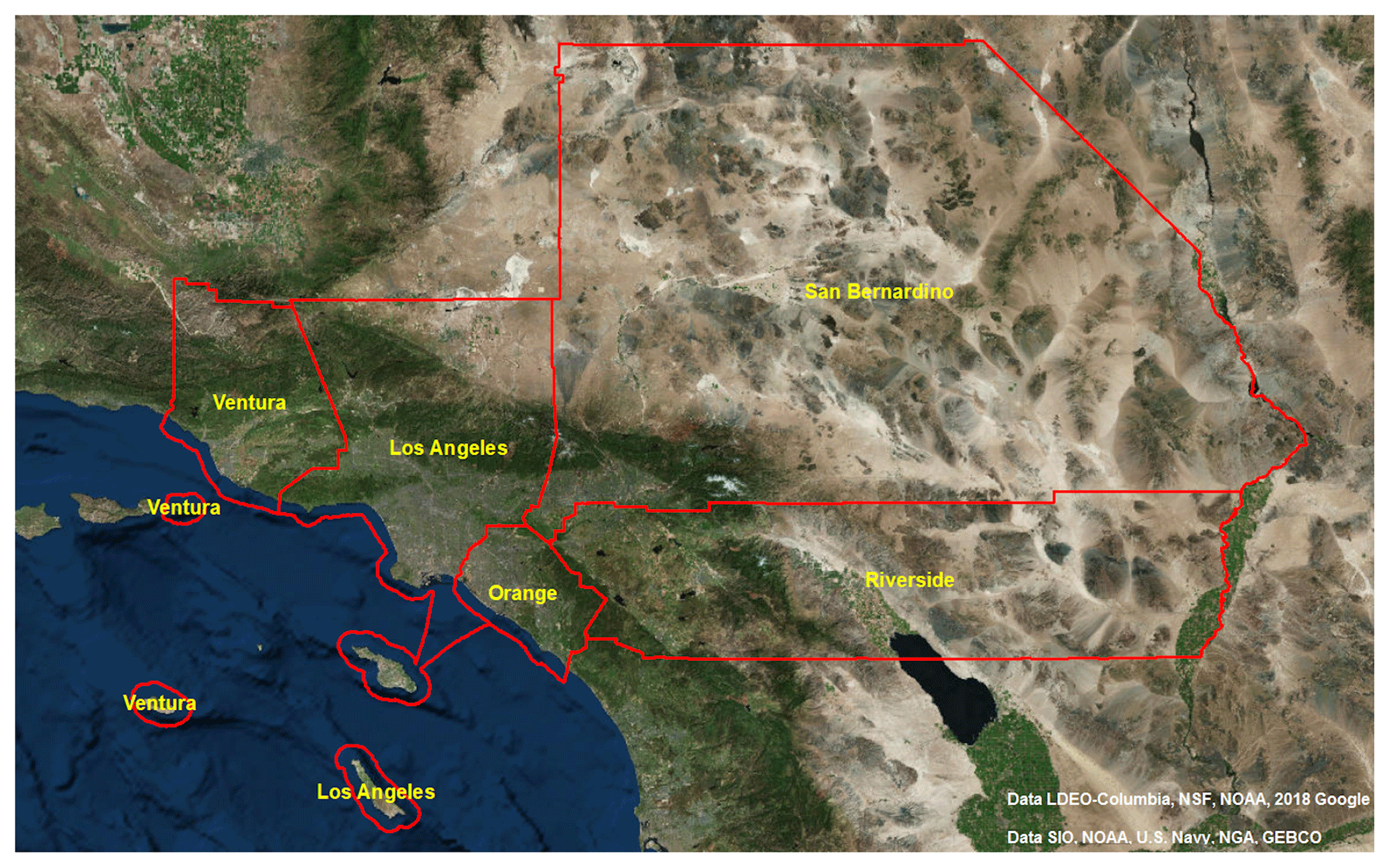
Figure 1The Hestia-LA urban domain. © Google Maps.
Because urban areas differ in key attributes such as size, geography, and emission sector composition, multiple cities are now being used to test aspects of anthropogenic CO2 monitoring and modeling. For example, ongoing efforts in integration of atmospheric measurements and bottom-up emissions information are taking place in Paris (Bréeon et al., 2015; Staufer et al., 2016), Boston (Sargent et al., 2018), Salt Lake City (Mitchell et al., 2018) and London (Font et al., 2015), to name a few. The Hestia approach has been used in a number of these urban domains. Here, we provide the methods and results from one of those urban domains, the Los Angeles Basin megacity. The Hestia-LA effort was developed under the Megacities Carbon framework (https://megacities.jpl.nasa.gov/portal/, last access: 12 August 2019). It was designed to serve the Megacities Carbon Project in a similar capacity to its role in INFLUX. The Hestia-LA results are unique in that they give us the first high-resolution spatiotemporally explicit inventory of FFCO2 emissions centered over a megacity. A preliminary version of Hestia-LA containing only the transportation sector emissions was reported by Rao et al. (2017). While emphasis thus far has been focused on atmospheric CH4 monitoring analyses in the LA megacity (Carranza et al., 2018; Wong et al., 2016; Verhulst et al., 2017; Hopkins et al., 2016), work is ongoing to use the extensive atmospheric CO2 observing capacity in the Los Angeles domain (e.g., Newman et al., 2016; Feng et al., 2016; Wong et al., 2015; Wunch et al., 2009) within an atmospheric CO2 inversion (i.e., an approach whereby CO2 concentration measurements in the atmosphere are combined with models of wind motions to infer what the emissions emanating from the surface must be).
In this paper, we describe the study domain, the input data, uncertainty, and the methods used to generate the Hestia-LA (v2.5) data product and provide descriptive statistics at various scales of aggregation. We compare the Hestia results to the metro region planning authority estimate and place the results in the context of urban greenhouse gas mitigation. We discuss known gaps and weaknesses in the approach and goals for future work.
2.1 Study domain
The Los Angeles metropolitan area is the second-largest metropolitan area in the United States and one of the largest metropolitan areas in the world. Under the definition of the Metropolitan Statistical Area (MSA) by the U.S. Office of Management and Budget, Metropolitan Los Angeles consists of Los Angeles and Orange counties with a land area of 12 562 km2 and a population of 9 819 000. The Greater Los Angeles Area, as a Combined Statistical Area (CSA) defined by the U.S. Census Bureau, encompasses the three additional counties of Ventura, Riverside, and San Bernardino, with a total land area of 87 945 km2 and an estimated population of 18 550 288 in 2014. The Hestia-LA FFCO2 emissions data product covers the complete geographic extent of these five counties, including the eastern, relatively non-urbanized portions of San Bernardino and Riverside counties. Airport emissions associated with aircraft up to 914 m are included, as are marine shipping emissions out to 22.2 km from the coastal boundary. Emissions considered here are carbon dioxide only; other important greenhouse gases such as methane (CH4) and nitrous oxide (N2O) are not included.
2.2 Input data
Input data to the Hestia-LA data product are supplied by output of the Vulcan Project (Fig. 2), a quantification of FFCO2 emissions at fine spatial scales and timescales for the entire US landscape (Gurney et al., 2009). The Hestia-LA process extracts these results for the five counties within the Hestia-LA domain and adjusts these estimates where superior local data are available and further downscales and distributes the Vulcan v3.0 results to buildings and street segments. Details of the Vulcan v3.0 methodology are provided elsewhere (Gurney et al., 2018). Here, we summarize the Vulcan v3.0 methods and then provide greater detail regarding the Hestia-LA processing of that data to high-resolution spatial scales and timescales.
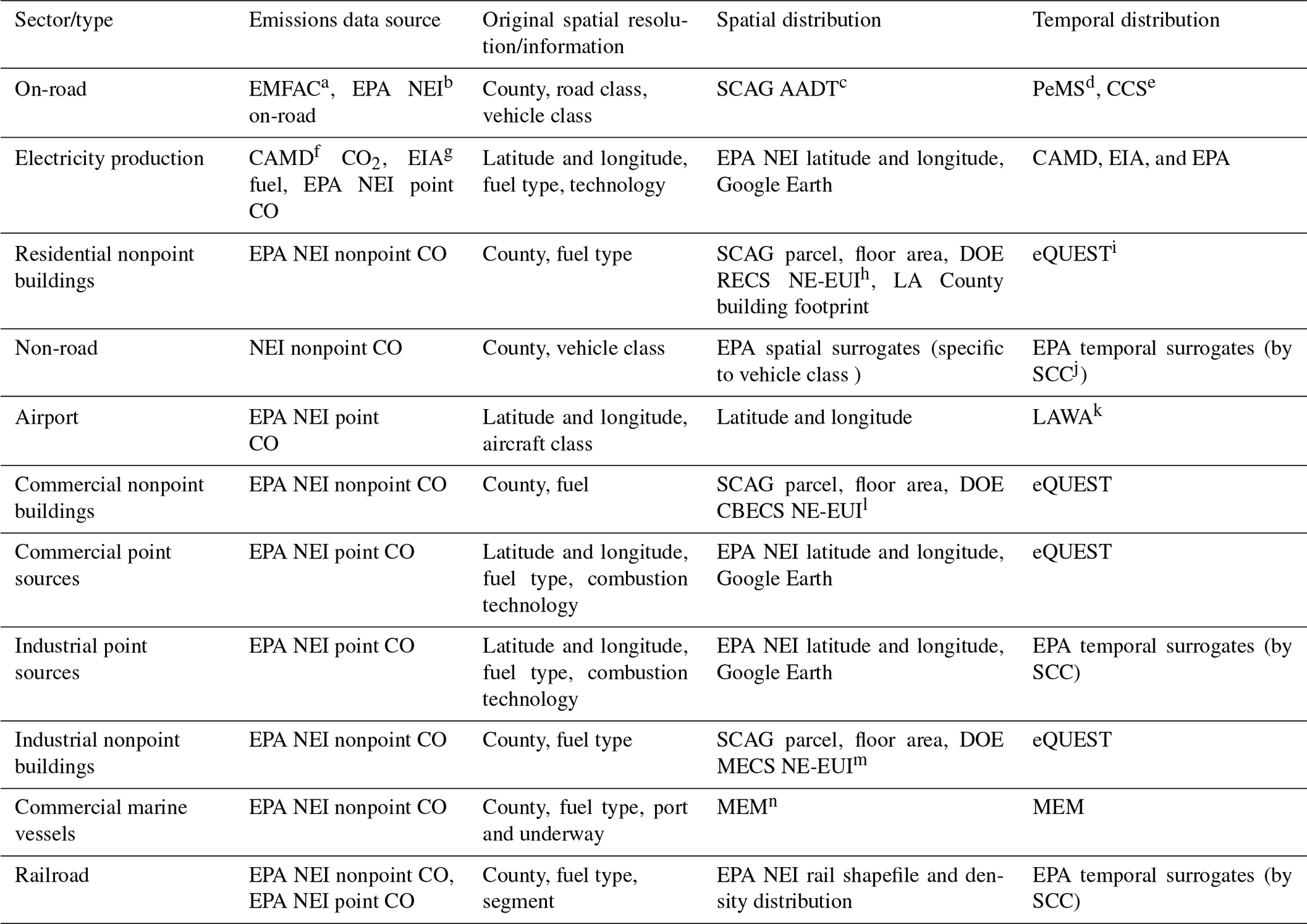
The Vulcan v3.0 input data (the output of which is the input for the Hestia-LA) are organized following nine economic sector divisions (see Table 1) – residential, commercial, industrial, electricity production, on-road, non-road, railroad, commercial marine vessel, and airport. Also included are emissions associated with the calcining process in the production of cement. The data sources within each sector are either acquired as FFCO2 emissions (the on-road sector and most of the non-road and electricity production sectors) or as carbon monoxide (CO) emissions (all other sectors) and transformed to FFCO2 emissions via emission factors. Furthermore, the data sources are represented geographically as either geocoded emitting locations (“point”) or as spatial aggregates (“nonpoint” or area-based emissions). Point sources are stationary emitting entities identified with geocoded locations such as industrial facilities in which emissions exit through a stack or identifiable exhaust feature (USEPA, 2015a). Area or nonpoint source emissions are not inventoried at the facility level but represent diffuse emissions within an individual US county. Because the focus of the current study is CO2 emissions resulting from the combustion of a fossil fuels, fugitive or evaporative emissions are not included and neither are “process” emissions, for example, associated with high-temperature metallurgical processes. Similarly, emissions associated with waste decay (organic or inorganic) are not included.

Figure 2Total annual FFCO2 emissions for the year 2011 from the Vulcan v3.0 output.
Much of the input data for Vulcan v3.0 are acquired from the Environmental Protection Agency's (EPA) National Emission Inventory (NEI) for the year 2011 (referred to hereafter as the “2011 NEI”), which is a comprehensive inventory of all criteria air pollutants (CAPs) and hazardous air pollutants (HAPs) across the United States (USEPA, 2015b). All of the individual record-level reporting in the 2011 NEI comes with a source classification code (SCC) that codifies the general emission technology, fuel type used, and sector (USEPA, 1995).
FFCO2 emissions from the electricity production sector are primarily retrieved from two sources other than the 2011 NEI. The first is the EPA's Clean Air Markets Division (CAMD) data (USEPA, 2015c), which reports FFCO2 emissions at geocoded electricity production facility locations. The second is the Department of Energy's Energy Information Administration (DOE EIA) reporting data (DOE/EIA, 2003), which reports fuel consumption at geocoded electricity production facility locations. Some electricity production emissions are retrieved from the 2011 NEI (as CO emissions). Overlap between these three data sources is eliminated via preference in the order listed above. A detailed comparison made between the CAMD and EIA FFCO2 emissions, along with greater detail regarding data sources, processing, and procedures can be found in Quick (2014) and Gurney et al. (2014, 2016, 2018).
The 2011 on-road FFCO2 emissions are retrieved from the EMissions FACtors 2014 model (EMFAC2014), produced by the California Air Resources Board (CARB, 2014). On-road transportation represents all mobile transport using paved roadways and includes both private and commercial vehicles of many individual classes (e.g., passenger vehicles, buses, light duty trucks, etc). The non-road sector, by contrast, includes all surface mobile vehicles that do not travel on designated paved road surfaces and a large class of vehicles such as construction equipment (e.g., bulldozers, backhoes, etc.), ATVs, snowmobiles, and airport fueling vehicles. The non-road emissions are derived from the 2011 NEI reporting of non-road CO emissions. Airport emissions include all the emissions emanating from aircraft during their taxi, takeoff, and landing cycles up to 914 m and are derived from the 2011 NEI point reporting. Other activities occurring at airports resulting in FFCO2 emissions are captured in the commercial building sector (building heating) or the non-road sector (baggage vehicles), sourced to the 2011 NEI nonpoint, 2011 NEI point, and 2011 NEI non-road reporting. Railroad emissions include passenger and freight rail travel and are sourced to the 2011 NEI nonpoint and point reporting. Commercial marine vessels (CMV) include all commercial-based aquatic vessels on either ocean or freshwater, sourced to the 2011 NEI nonpoint reporting. Personal aquatic vehicles such as pleasure craft and sailboats are included in the non-road sector. Emissions associated with cement calcining are included given its potential size and the tradition of including it with CO2 inventories and use information from multiple sources (PCA, 2006; USGS, 2003; IPCC, 2006).
The FFCO2 emissions input to the Hestia system from the Vulcan v3.0 output is associated with spatial elements represented by points, lines, and polygons, depending upon the data source, the sector, and the available spatial proxy data (Table 1). Further spatialization and temporalization occurs in the Hestia system.
Table 1Data sources used in the spatiotemporal distribution of FFCO2 emissions (the text provides acronym explanations and sources).
a Emissions Factors Model.
b Environmental Protection Agency, National Emissions Inventory.
c Southern California Association of Governments, annual average daily
traffic.
d Performance measurement system.
e Continuous count stations.
f Clean Air Markets Division.
g Energy Information Administration.
h Department of Energy Residential
Energy Consumption Survey, nonelectric
energy use intensity.
i Quick Energy Simulation Tool.
j Source classification code.
k Los Angeles World Airport.
l Department of Energy Commercial Energy Consumption Survey, nonelectric
energy use intensity.
m Department of Energy Manufacturing Energy Consumption Survey,
nonelectric energy use intensity.
n Marine Emissions Model.
To estimate FFCO2 emissions as a multiyear time series from 2010 to 2015, the results for the year 2011 were scaled using sector, state, and fuel consumption data (thermal units) from the DOE EIA (DOE/EIA, 2018). The electricity production sector was an exception to this approach where year-specific data were available in the CAMD and EIA data sources. Ratios were constructed relative to the year 2011 in all SEDS sector designations for each US state. The ratio values are applied to the annual totals in each of the sector and fuel categories specific to the state FIPS code.
2.3 Space and time processing
2.3.1 Residential, commercial, and industrial nonpoint buildings
The general approach to spatializing residential, commercial, and industrial nonpoint FFCO2 emissions is to allocate the county-scale, fuel-specific annual sector totals to individual buildings (or parcels) using data on building type, building age, total floor area, energy use intensity, and location.
A portion of the Hestia-LA building information was provided by the Southern California Association of Governments (SCAG) (Kimberly S. Clark and Christine Fernandez, Southern California Association of Governments, personal communication, 2012) and included building type, age, floor area, and location. The spatial resolution of this information was at the land parcel scale (larger than the building footprint). Building footprint data were available in the county of Los Angeles only, which offered additional building floor area information needed to correct some floor area values in the SCAG parcel data (LAC, 2016). For example, a large number of commercial parcels with zero floor area were found in the Riverside County data, which were visually inspected in Google Earth to include qualifying buildings. These floor area values were corrected through the combination of the census block-group General Building Stock (GBS) database from the Federal Emergency Management Agency (FEMA) (FEMA, 2017) and the National Land Cover Database 2011 (NLCD), which classifies the US land surface in 30 m pixels (Homer et al., 2015).
Building energy use intensity was derived from data gathered by the DOE EIA and the California Energy Commission (CEC). The DOE EIA Commercial Buildings Energy Consumption Survey (CBECS), Manufacturing Energy Consumption Survey (MECS), and Residential Energy Consumption Survey (RECS) represent regional surveys of building energy consumption categorized by building type, fuel type, and age cohort (RECS, 2013; CBECS, 2016; MECS, 2010). Data for the Pacific West Census Division was used and in the case of the commercial sector, was appended by the CECs Commercial End-Use Survey (CEUS) data (CEC, 2006).
In the residential sector the nonelectric energy use intensity (NE-EUI) was calculated from the reported energy consumed and total floor area sampled specific to five building types (Table 2) in the 2009 RECS survey. This was additionally categorized by fuel type (natural gas and fuel oil) and two age cohorts (pre-1980 and post-1979).
Table 2Residential NE-EUI survey values by building type from the Residential Energy Consumption Survey (RECS).
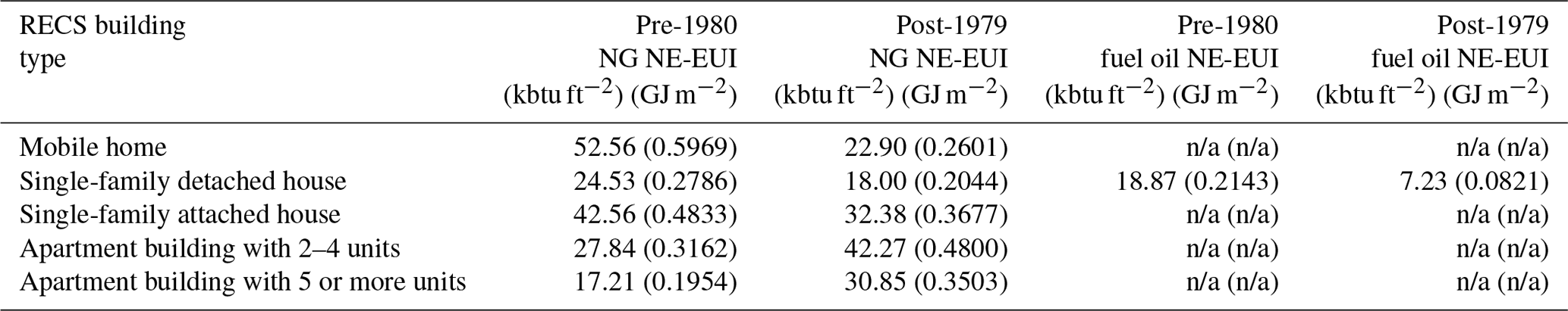
“n/a” – not applicable. This indicates that there was no fuel consumption of this type evident from the survey data.
In the commercial sector, the NE-EUI was similarly calculated from the 2012 CBECS energy consumption micro-data and total floor area sampled specific to 20 building types, two fuel types (natural gas and fuel oil), and two age cohorts (pre-1980 and post-1979). However, the sampling for the two age cohorts was insufficient to generate estimates and the age distinction was eliminated. Furthermore, where the sample sizes remained small, NE-EUI data from the CEUS was used in place of CBECS estimates (7 of 20 building types qualified). As the CEUS follows a building typology different from CBECS, a relationship of building types between the two datasets was necessary (Table 3).
Table 3Building type relationship and NE-EUI values for commercial buildings derived from the CBECS and CUES databases.

* NE-EUI uses the CUES NE-EUI value due to sampling limitations in the CBECS data.
Unlike the commercial and residential survey data, the 2010 MECS survey data do not quantify energy consumption for individually sampled buildings but rather report the sum of the sampled buildings within each census region categorized by manufacturing sector. The resulting NE-EUI values are shown in Table 4. Like the commercial data, there was inadequate sampling to justify two age cohorts.
Table 4Industrial NE-EUI survey values from the DOE EIA MECS database.
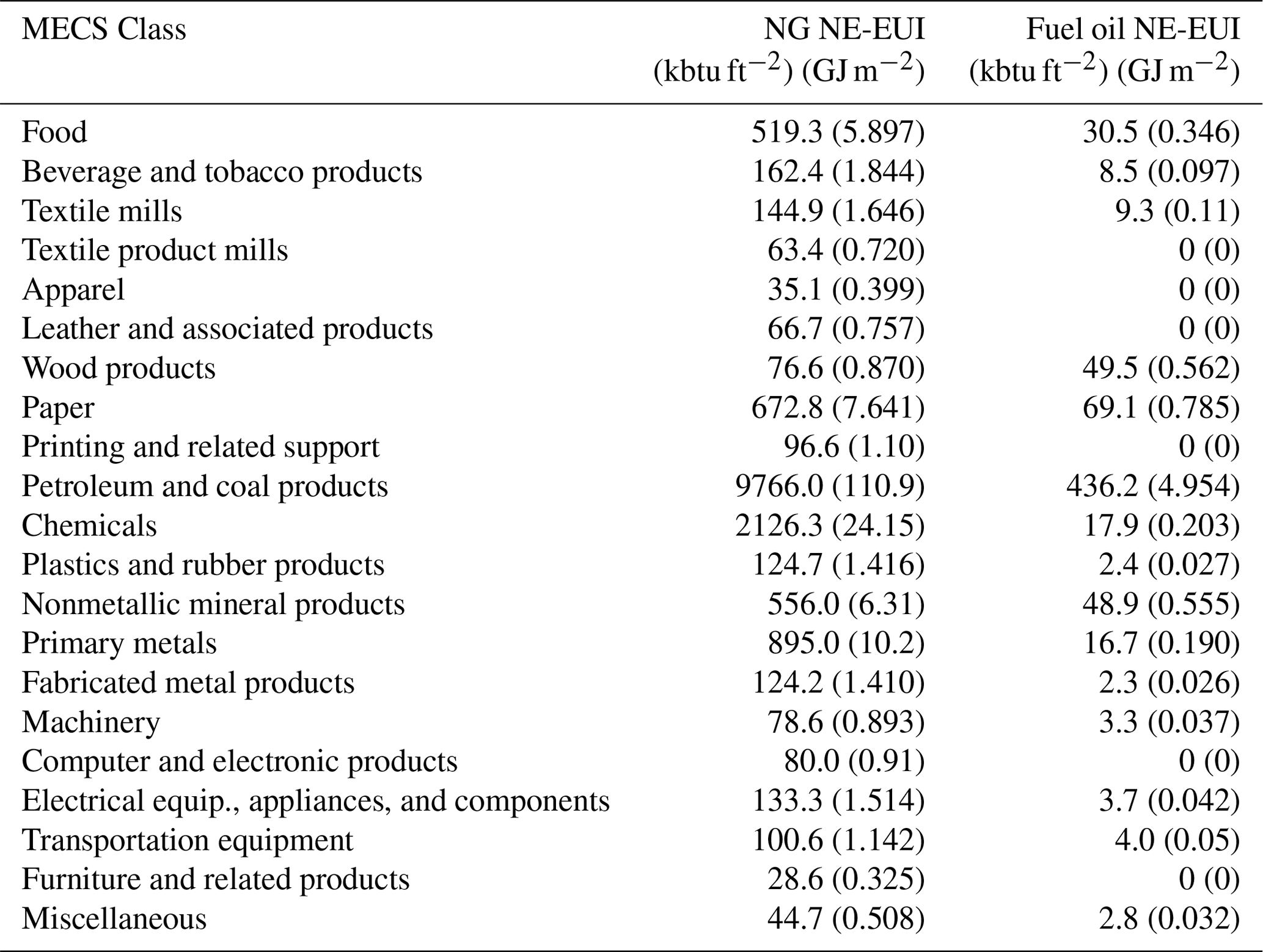
The NE-EUI values derived from the CBECS/RECS/MECS and CEUS survey data reflect the total building fuel consumption for a specific fuel in a census region divided by the total floor area of all buildings in that census region consuming that fuel. This generates a mean building NE-EUI value. Actual buildings will vary around that mean value for a variety of reasons including different occupancy schedules, different energy efficiencies (in the envelope or heating and cooling system), different microclimate, and other physical and behavioral characteristics. Furthermore, the NE-EUI value applied in this way will not capture the reality that some buildings do not use fossil fuel (electricity-only buildings) or that some buildings use one fossil fuel only versus another or use a mix of fuels in a proportion different from the county total. Hence, each building will be allocated a mix of fossil fuel consumption identical to the county total.
Spatial distribution
The county-scale commercial, residential, and industrial nonpoint FFCO2 emissions are allocated to each land parcel in proportion to the product of the NE-EUI and the total floor area,
where the energy consumed, EC, in each building, b, is the product of the NE-EUI value, NE_EUI, and the floor area, FA, for each fuel, f, and each building in sector, s. The total energy consumed, TEC, within the county for a sector, s, is the sum of all the EC values across the N buildings in the sector,
To convert this to FFCO2 emissions, we first calculate the fraction of the total energy consumption associated with each building,
where F is the fraction of TEC consumed in building, b, of sector s. This is then used to distribute the county total FFCO2 emissions as follows:
where E is the FFCO2 emissions either for the county or for building, b, and fuel. In allocating emissions from coal consumptions, however, NE-EUI takes the value of “1” for all building types so that the allocated emission in a building is directly proportional to the floor area.
Temporal distribution
The hourly time structure for buildings in the residential and commercial sectors are created via the use of eQUEST, a building energy simulation tool run for each of the building classes listed in Tables 2 and 3 and using only the temporal structure of the energy consumption output (Hirsch and Associates, 2004). The model domain is specified as the city of Los Angeles for the year 2011 with Typical Meteorological Year (TMY) weather data from the DOE (Marion and Urban, 1995). The mean building area is provided by the parcel data as described previously.
For the industrial buildings, a temporal profile representing the mean of industrial point source temporal surrogates provided by EPA, are used (USEPA, 2015a). Figure 3 shows the hourly time profile during a 1-week period in April for a selected building in the residential and commercial sector.
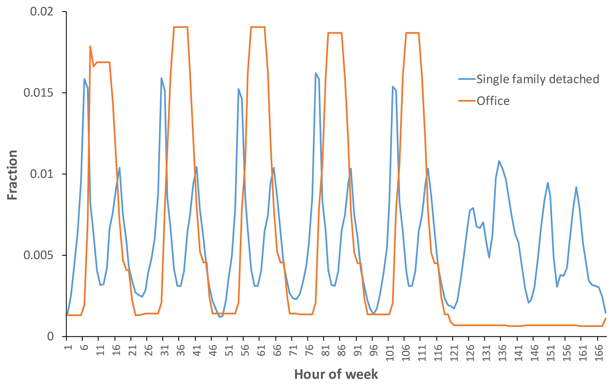
Figure 3Energy consumption intensity (hourly fraction) from an eQUEST simulation of the average week in 2011 for two types of buildings: “single-family detached house” and “office”.
2.3.2 Industrial and commercial point sources
Little space and time processing is required for industrial and commercial point source emissions since they are geocoded to specific facilities and emitting stacks or similar identifiable emission points. However, visual inspection of the point source locations in Geographical Information System (GIS) suggested potential geocoding errors. Point source locations were reviewed by searching facility names to an online address search or via the EPA's Facility Registry Service (FRS), which can link the facility in question to all the reporting made to the federal government under other environmental regulations (USEPA, 2013). This often returns a more accurate physical location. The geolocations considered inaccurate were manually corrected. Out of the total 192 facilities with corrected locations, 13 were moved a distance of between 924 and 1022 km, while the remaining 179 were moved 0.5 km or less. The large magnitude location changes were likely transcription errors when originally recording the location coordinates.
A given commercial or industrial point source is typically composed of multiple emission processes or units. For example, in Los Angeles County, the 2011 NEI reports a total of 3409 emission records at 842 individual facilities. In some cases, the multiple emitting points at a facility are not at exactly the same geocoded point but may represent different emitting points at a facility that occupies a large area of land. Most often, however, all emitting points at a given facility are geocoded to the same latitude and longitude.
The sub-annual temporal distribution for the commercial and industrial point source emissions used temporal surrogate profiles provided by the EPA, linked according to the SCC of the emission record (USEPA, 2015a).
2.3.3 Electricity production
As described in Sect. 2.2, three different data sources are used to quantify the FFCO2 emissions in the Hestia-LA domain: the Clean Air Markets Division (CAMD), the DOE-EIA reporting, and 2011 NEI CO emissions data. In 2011 there were a total of 34 CAMD facilities, 228 EIA facilities and 147 NEI facilities (reported through the NEI 2011 point source file set) in the Hestia-LA domain. Total electricity production emissions in the domain were 6.21 MtC yr−1 exclusive of biogenic fuels and 6.68 MtC yr−1 with biogenics included. The CAMD data are reported at an hourly resolution, while the DOE EIA data are reported at a monthly resolution and the 2011 NEI data are reported at an annual resolution only. Reduction of all data to an hourly time increment was achieved by maintaining constant emissions within a month or year for the DOE EIA and 2011 NEI data, respectively.
2.3.4 On-road emissions
A preliminary version of the Hestia-LA on-road emissions estimates were presented by Rao et al. (2017). The version presented here uses updated data and Hestia methodologies.
Temporal distribution
The Hestia-LA on-road FFCO2 emissions input are retrieved from the Vulcan v3.0 output spatialized to specific road segments in the Hestia-LA domain and categorized by vehicle class and fuel. Hence, no further spatialization was required.
Construction of the temporal distribution in the Hestia system relies upon the California Department of Transportation (CalTrans) Performance Measurement System (PeMS) (PeMS, 2018). This dataset contains 2011 traffic count data collected at 5 min intervals at measuring stations along freeways and principal arterials and along some minor arterials and collectors (major and minor). Aggregation of the 5 min counts to hourly values are used to construct hourly fractions for each measurement station.
To apply a time distribution for the FFCO2 on-road emissions on each road segment, an inverse distance weighting (IDW) spatial interpolation method was used. A search within a neighborhood of a 10 km radius was performed from the midpoint of each road segment to locate PeMS sites using a nearest neighbor searching library (Mount and Arya, 2010). In cases where more than one station was available, the IDW interpolation was applied; in cases where only one station was available, the time structure of this station was directly assigned to the road segment in question. In cases where no station was available within the 10 km neighborhood, an average temporal distribution was assigned (an average of all station values in a county at that hour for that road type). This last case occurred mostly in the rural portions of predominantly rural counties.
For local roads, PeMS data were not available in any of the counties within the Hestia-LA domain. Instead, the weekday hourly time fractions were generated from Annual Average Weekday Traffic (AAWT) data supplied by SCAG (Mike Ainsworth and Cheryl Leising, Transportation Planning Department, SCAG Riverside Office, personal communication, 2014). The data contained five distinct time periods within a single 24 h cycle: 06:00–09:00, 09:00–15:00, 15:00–19:00, 19:00–21:00, 21:00–06:00. Hourly time fractions for weekends were derived from the county average of weekend hourly time fractions. The weekday and weekend hourly time fractions were combined to form a complete week, and then replicated for all 52 weeks in the entire year. This was done because there was no significant seasonality in weekday and weekend traffic across the year as observed from PeMS data.
2.3.5 Non-road
The non-road Hestia-LA FFCO2 emissions are completely determined in the Vulcan system, and hence passed to the Hestia-LA domain without further processing (see Gurney et al., 2018 for details). To summarize the Vulcan process, California did not report FFCO2 non-road emissions to the NEI 2011 but did report non-road CO emissions. The CO emissions were converted to FFCO2 using the SCC-specific ratios of CO2∕CO derived from all other states that reported both species (a mean value). The spatial distribution of the non-road FFCO2 emissions followed two approaches. Non-road FFCO2 emissions reported through the 2011 NEI point data source (five locations, 12 % of non-road FFCO2 in the LA megacity) are located in space according to the provided latitude and longitude. Emissions reported through the county-scale non-road data source utilize multiple spatial surrogates provided by the EPA, reflecting a series of spatial entities such as the mines, golf courses, and agricultural lands. There were instances in which non-road FFCO2 emissions could not be associated with a spatial entity due to missing data. These emissions are spatialized by first aggregating all the offending sub-county emission elements within a county for a given surrogate shape type (e.g., golf courses, mines) and then distributing these emissions evenly across the county.
To distribute the non-road FFCO2 emissions from the annual to hourly timescale, a series of surrogate time profiles provided by the EPA are used. These temporal surrogates are comprised of three cyclic time profiles (diurnal, weekly, monthly) specific to SCC that are combined to generate hourly SCC-specific time fractions for an entire calendar year.
2.3.6 Airport
Emissions of FFCO2 from airports retrieved from the Vulcan system for the Hestia-LA domain are specific to geocoded airport locations. Hence, the Hestia-LA system performs the temporal distribution only. There are 374 commercial airports and helipads in the Hestia-LA domain totaling 0.77 MtC yr−1, dominated by Los Angeles County (0.39 MtC yr−1), and LAX in particular.
The annual airport FFCO2 emissions are distributed in time utilizing airport-specific flight volume data from four datasets:
-
the Operations Network (OPSNET) data from the Federal Aviation Administration (FAA), which reports total date-specific daily flight volume (365 values) at specific airports for specific aircraft classes (FAA, 2018a);
-
“AIRNAV” data that reports average daily percentage flight volume for aircraft class at US airports and facilities (AirNav, http://www.airnav.com/airports/, last access: 1 August 2018);
-
the Enhanced Traffic Management System Count (ETMSC) daily flight volume data from the FAA for two airports' in the Hestia-LA domain (NTD and RIV) with mostly military operations (FAA, 2018b);
-
the Los Angeles World Airport (LAWA) data, which reports hourly flight volume for Los Angeles International Airport (LAX), Ontario Airport (ONT), and Van Nuys Airport (VNY) (Norene Hastings, Environmental Supervisor, Environmental Services division, Los Angeles World Airports, personal communication, 2014).
For three large airports (LAX, ONT, VNY), the daily aircraft class-specific flight volume (from OPSNET) and the hourly data of flight volume (from LAWA) were combined to create hourly aircraft class-specific time profiles (Figs. 4–6). All of the flight volume data are specific to four aircraft classes: Military (MIL), Air Carrier (AC), General Aviation (GA), and Air Taxi (AT).
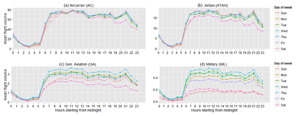
Figure 4Average hourly flight volume at LAX for (a) total, (b) AC, (c) AT, (d) GA, and (e) MIL aircraft classes for each day of the week. The plots represent the mean diurnal cycle for all Mondays, Tuesday, Wednesdays, and so on, given a full year of data.
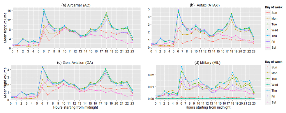

To generate hourly time profiles for all other airports in the Hestia-LA domain for which this type of detailed hourly data were not available, airports first were categorized based on average daily flight volumes and average aircraft class proportions from the OPSNET, AIRNAV and ETMSC data. Each airport was categorically matched to one of the two non-international airports with hourly data (ONT, VNY) and the hourly time fractions adopted. LAX was unique in terms of its volume and aircraft class proportions and hence was not used for any other airports. For helipads and very small airports, a flat time structure was used.
2.3.7 Railroad
Railroad FFCO2 emissions are similarly distributed in space within the Vulcan system and passed through to the Hestia-LA landscape without alteration (see Gurney et al., 2018 for additional details). The Vulcan process treats railroad point records somewhat differently from the railroad nonpoint records. The point source railroad emissions are associated with rail yards and related geo-specific locales and are placed in space according to the provided latitude and longitude. The railroad FFCO2 emissions associated with the nonpoint 2011 NEI reporting contain an ID variable that links to a spatial feature (rail line segment) in the EPA railroad GIS shapefile. Nearly two-thirds of the railroad emitting segments have no segment link. The sum of these “unlinked” railroad FFCO2 emissions are distributed to rail line within the given county according to freight statistics. The annual railroad FFCO2 emissions are distributed to the hourly timescale with no additional temporal structure (a “flat” time distribution).
2.3.8 Commercial marine vessels
The commercial marine vessel (CMV) FFCO2 emissions retrieved from the Vulcan system are specific to county and SCCs, which are subsequently aggregated by the Hestia-LA system into emissions associated with two activity categories: “port” emissions and “underway” emissions. For the port CMV emissions (Fig. 7), a port shapefile from the EPA was used as a reference along with a visual inspection of the coastline (USEPA, 2015a).
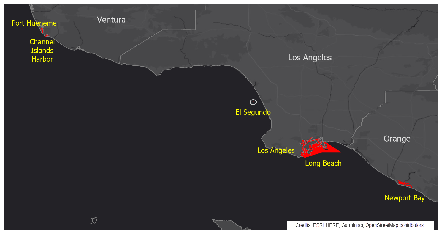
Figure 7The six ports in the Hestia-LA domain to which Vulcan FFCO2 port emissions are allocated. © OpenStreetMap contributors 2019. Distributed under a Creative Commons BY-SA License.
Allocation of the FFCO2 emissions designated as “underway” used a polyline shapefile (Fig. 8) of commercial shipping lanes in California provided by CARB (Andy Alexis, California Air Resources Board, personal communication, 2011, https://www.arb.ca.gov/ports/marinevess/ogv/ogv1085.htm, last access: 6 July 2011). The shipping lanes for each county were bounded so that only lanes between the exterior of ports and a distance of 38.6 km from the port exterior were included. County total FFCO2 emissions were then distributed evenly to these shipping lanes on a per unit length basis individually for each of the three counties. Each shipping lane segment receives its length fraction of the annual total of underway emissions.
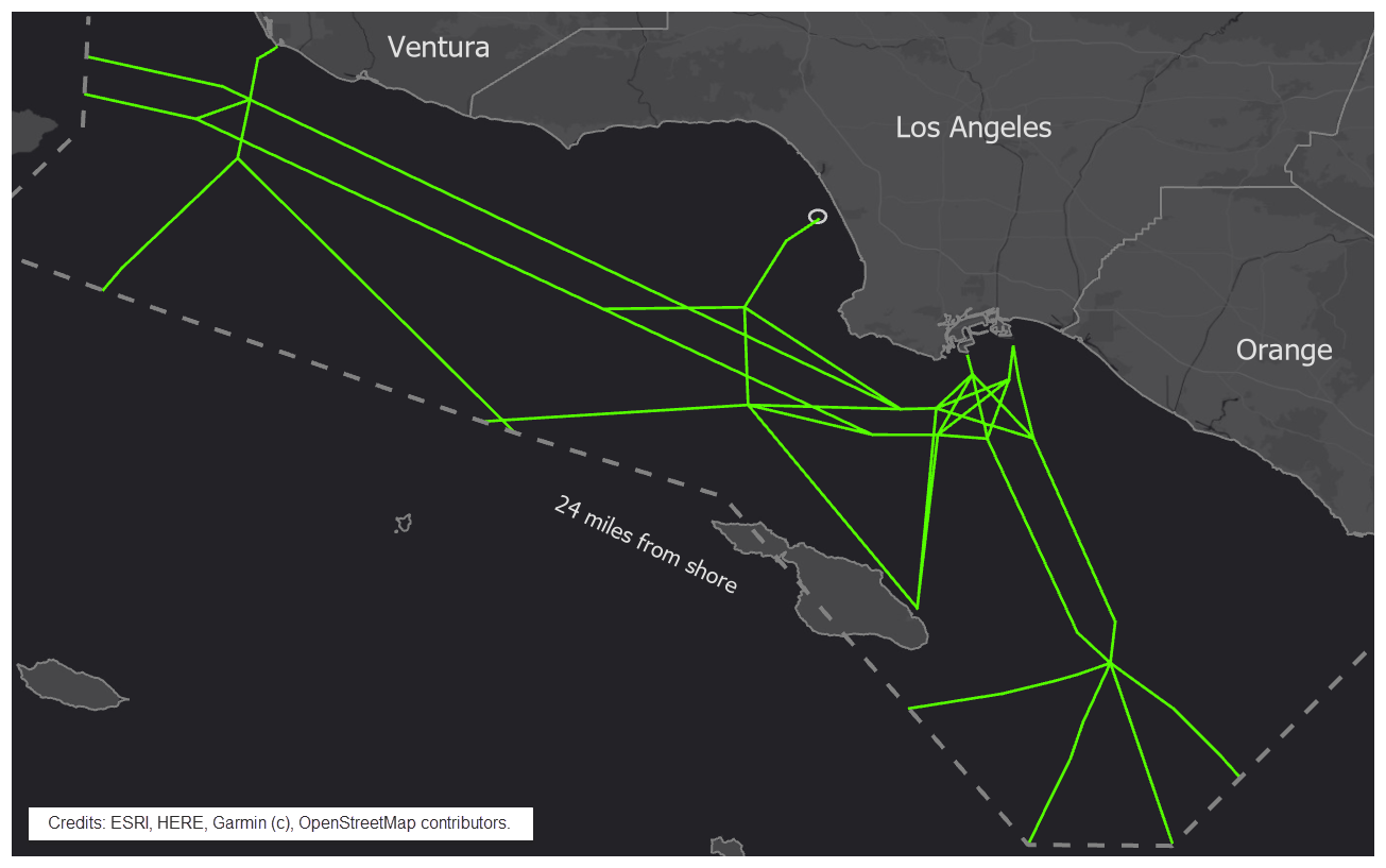
Figure 8Commercial Marine Vessel (CMV) shipping lanes in Hestia-LA to which Vulcan FFCO2 underway emissions are allocated (24 miles = 38.6 km). © OpenStreetMap contributors 2019. Distributed under a Creative Commons BY-SA License.
The time profile was based on the Marine Emissions Model (MEM) developed by CARB. MEM had marine vessel activity data, which includes the arrival time of ocean-going vessels for all ports in California spanning the 2004 to 2006 time period (Andy Alexis, California Air Resources Board, personal communication, 2011). This hourly dataset was analyzed using a Fourier time series, which allowed for an isolation of the dominant cycles of ship traffic in the data. Results from the Fourier fit were then used to fill in the missing hours. Weekday hours were examined separately from weekend hours to isolate potential differences in traffic volume. Three cycles resulted: a 24 h diurnal cycle, a weekly cycle, and a monthly cycle. These were applied to all years of the annual FFCO2 emissions to create an hourly distribution at each of the CMV ports within the domain.
2.3.9 Cement
Emissions of FFCO2 from cement production facilities retrieved from the Vulcan system for the Hestia-LA domain are specific to geocoded facility locations. CO2 is emitted from cement manufacturing as a result of fuel combustion and as process-derived emissions (Andrew, 2018). The emissions from fuel combustion are captured in the industrial sector. The process-derived CO2 emissions result from the chemical process that converts limestone to calcium oxide and CO2 during “clinker” production (clinker is the raw material for cement, which is produced by grinding the clinker material). These emissions are reported as cement sector emissions.
These emissions are fully calculated, spatialized and temporalized in the Vulcan v3.0 system and passed directly to the Hestia-LA landscape. The cement facilities are geocoded with some corrections to provide more accurate placement of the emission stacks.
2.4 Gridding
The county-level FFCO2 emissions inventory, which has been distributed into the point, line, and polygon features by sector, is rasterized into a sector-specific and time-resolved into gridded form under a common grid reference. This grid reference divides the entire Hestia-LA domain into 509 by 342 1 km × 1 km grid cells on the California State Plane Coordinate System. The grid reference is made into “fishnet” in the shapefile format with 509 × 342 grid cells.
The first step of the gridding procedure is to perform a spatial intersection operation between the fishnet and each of the sectoral emissions layers in ArcGIS. The output of an intersection operation is a new set of features common to both input layers. The emissions value of each feature in the intersection output was scaled by the ratio of the spatial footprint of the feature to that of the original feature in the sectoral emissions layer. For line-sourced and polygon-sourced emissions layers, the spatial footprint represents the line length and polygon area, respectively. For point-sourced layers, the footprint is equal to 1.
2.5 Uncertainty
Uncertainty estimation for Hestia results is challenging owing to the fact that many of the datasets used to construct the flux results are not accompanied by uncertainty or traceable to transparent sources or methods. The approach taken for the Hestia-LA v2.5 results was to conservatively estimate the uncertainty based on available comparisons to Hestia results and exploration of the dominant components of the Hestia output. The first of these is a comparison of the Hestia-Indianapolis (Hestia-Indy) results to an inverse estimation of fluxes in the INFLUX project (Gurney et al., 2017). In that study, it was shown that the Hestia-Indy whole-city FFCO2 emissions result agreed with an inverse estimate (Lauvaux et al., 2016) within 3.3 % (CI: −4.6 % to +10.7 %). This suggests both potential bias (3.3 %) and an estimation uncertainty (∼7.5 %). This comparison was accomplished by estimating portions of the carbon budget, included in the inverse estimate but not explicitly included in the Hestia-Indy result. Most importantly, biosphere respiration estimated from chamber studies at commensurate urban latitudes was combined with a remote-sensing based approach to quantifying the available vegetated landscape. This comparison, it should be noted, is for a single city (Indianapolis) for a single time period. We directly sum the random and systematic error and use this in the current study to represent the Hestia-LA whole-city uncertainty (a 95 % CI), rounded up to 11 %.
The next element for consideration with a conservative uncertainty estimate is the work done to compare two different electricity production FFCO2 estimates in the US. This work (Gurney et al., 2016) found that one-fifth of the facilities had monthly FFCO2 emission differences exceeding +6.8 % for the year 2009 (the closest analyzed year to the 2011 analysis examined here). The distributions of emissions of the two datasets were not normally distributed and neither were the differences. Hence, a typical Gaussian uncertainty estimate cannot be made – rather, the difference distribution was represented by quintiles of percentage difference. Hence, these values cannot be cast within the context of other normally distributed errors. However, we conservatively consider the quintile value (the positive and negative tails) as a 1σ value and 13 % as a 2σ value. The contribution of electricity production is important to urban FFCO2 emissions uncertainty given how large power production can be within the total urban FFCO2 context. For example, in the Los Angeles megacity, electricity production accounts for 19 % of the total FFCO2 emissions. The percentage differences can act as a form of uncertainty at the point-wise or (conservatively) the grid-cell scale, though only representative of the type of uncertainties represented by electricity production point sources.
Finally, an initial assessment of the range of two critical parameters in the Vulcan–Hestia estimation is included as part of the conservative uncertainty estimation. The two critical parameters are the CO emissions factor and the CO2 emissions factor. Primarily for the CO EF, there is a range of potential values for each application (combination of fuel category and combustion technology) though that range is not represented by a well-populated distribution of values but rather a discrete set of values within the data sources described in Gurney et al. (2009). Furthermore, the expectation is that the CO EFs would not be normally distributed even if there were to be a well-populated distribution of values (i.e., many literature estimates of the same fuel and combustion technology) owing to the nature of CO emissions from fuel combustion. This is driven by both the variation in combustion conditions for a given fuel–technology combination and the variation is CO EF values across combustion technology. The distribution would likely be a positively skewed “heavy-tailed” or “long-tailed” distribution. For the current study, a range of the CO and CO2 EF values culled from the literature are conservatively assigned a 1σ uncertainty of 10 % or a 2σ value of 20 %. Like the electricity production analysis in the previous paragraph, the uncertainty associated with the CO and CO2 emission factors is a grid-cell-scale uncertainty (as opposed to whole city where error cancelation occurs) and is independent of the electricity production uncertainty estimate (the CO and CO2 EF values are not used in the electricity production sector but in the other point sources and nonpoint sources).
These latter two uncertainties are more representative of grid-cell-scale uncertainties and sum them in quadrature to arrive at a grid-cell-scale uncertainty (95 % CI) of 23.4 % or conservatively rounded to 25 %. Work is underway that includes a complete input parameter range for the Hestia emissions data results to more formally assign uncertainty at multiple scales.
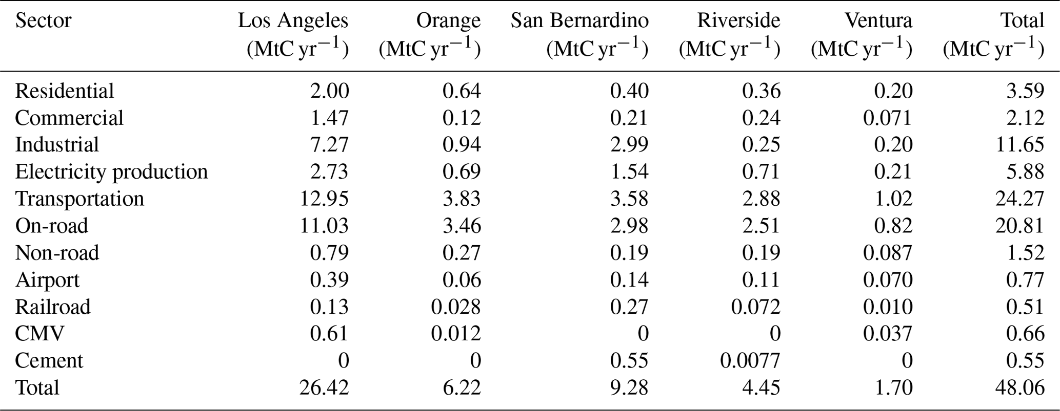
The total 2011 emissions for the Hestia-LA domain are 48.06±5.3 MtC yr−1 (Fig. 9, Table 5). Transportation accounts for the largest share (24.27±2.7 MtC yr−1) of the total, and within the transportation sector, on-road emissions account for the largest portion (20.81±2.3 MtC yr−1). The next largest sectors are the industrial (11.65 MtC yr) and electricity production (5.88±0.76 MtC yr−1) sectors. On-road, electricity production, residential, and industrial FFCO2 emissions make up 86 % of the total. Petroleum accounts for almost 75 % of the total LA megacity fuel consumption for direct FFCO2 emissions, consistent with the dominance of the transportation and industrial sectors, which are mostly reliant on petroleum fuels. Los Angeles County dominates emissions in the five counties of the Hestia-LA domain, accounting for 55 % of the total FFCO2 emissions. This is followed by San Bernardino, Orange, Riverside, and Ventura counties, respectively. Los Angeles and San Bernardino counties are dominated by on-road and industrial FFCO2 emissions, while on-road emissions account for the largest share in the remaining three counties by far. Not surprisingly, Los Angeles county has the largest CMV FFCO2 emissions among the five counties, owing to the port of Los Angeles, which hosts a large amount of international commercial shipping. At 0.61±0.067 MtC yr−1, it rivals in emission magnitude the combination of residential and commercial building emissions in each of the other four counties.

Figure 9Total FFCO2 emissions proportions for the Hestia-LA domain: (a) FFCO2 emission proportions by sector and (b) FFCO2 emission proportions by fuel category.
Table 5Sectoral FFCO2 emissions in the five Hestia-LA domain counties for the year 2011.
Total emissions in the LA megacity show a small downward trend over the 2010–2015 time period of 0.44 % yr−1, which is a statistically significant trend (slope: −0.21 MtC yr−1; CI: −0.397, −0.023). Individual sectors show greater variation and there are compensating temporal changes among the individual sectors (Fig. 10). The residential sector showed a relatively large decline in 2014, though due to its relatively small portion of total emissions, has limited impact on the total temporal variation from 2010–2015. Similarly, 2015 showed a large increase in commercial sector emissions, which also do not translate to large changes in the total FFCO2 emissions time series. The relative temporal stability of the industrial and on-road FFCO2 emissions sectors, combined with their large share of the total FFCO2 emissions, are reflected in the total emissions trend. When categorized by fuel type, natural gas FFCO2 emissions exhibited the greatest variation with a maxima in 2012 and to a lesser extent 2013, driven primarily by consumption in the electricity production sector.
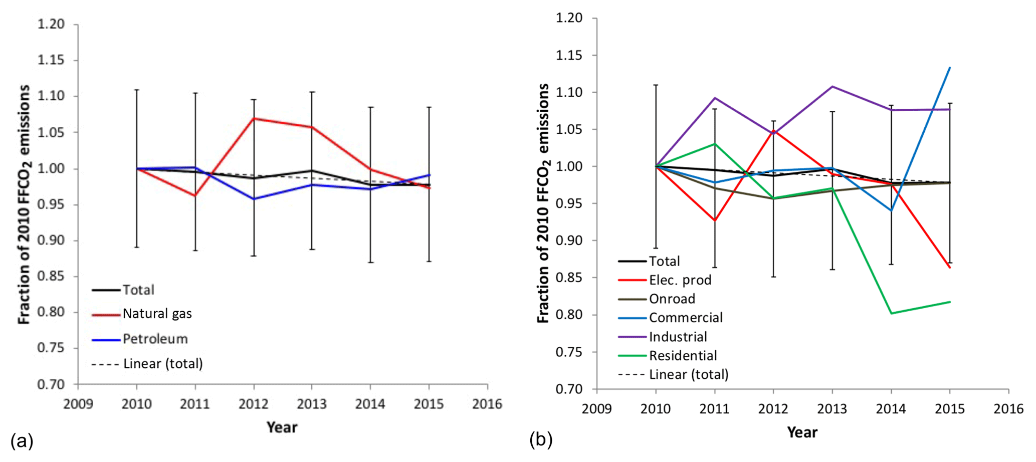
Figure 10Fractional changes over the 2010 to 2015 timeframe in LA Basin FFCO2 emissions: (a) by fuel category and (b) by sector. Whole-city error is provided for the total FFCO2 emissions only.
Spatial distribution of the Hestia-LA FFCO2 emissions demonstrates the importance of the populated areas and road-intensive portions of the domain in the overall emissions (Fig. 11). The constant emissions that appear over large areas, particularly in San Bernardino and Riverside counties, are due to the non-road FFCO2 emissions, which have relatively simple spatial distribution proxies with considerable areal extent.
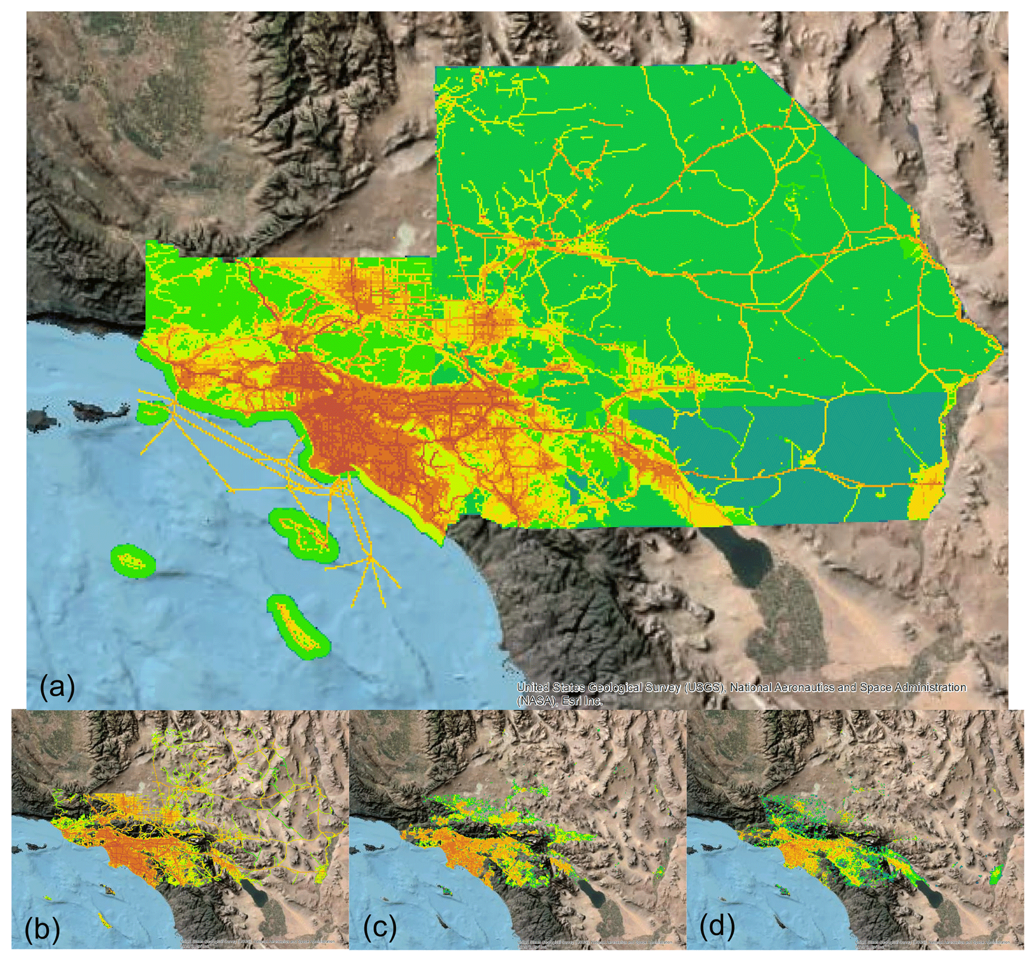
Figure 11Hestia-LA v2.5 FFCO2 emissions for the year 2011 represented on a 1 km × 1 km grid: (a) total FFCO2 emissions, (b) on-road FFCO2 emissions, (c) residential FFCO2 emissions, and (d) commercial FFCO2 emissions. Units: natural logarithm of kgC yr−1.
Figure 12 shows the cumulative FFCO2 emissions across four of the sectors for which the 1 km2 grid-cell accumulation is most appropriate: the commercial, industrial, on-road, and residential sectors. The other FFCO2 emission sectors (airport, electricity production, cement) are not included in Fig. 12 because they are dominated by a few points, have limited spatial distribution (railroad), or no spatial variance (non-road). The accumulation of FFCO2 emissions at the threshold by which 10 % of the grid cells are accumulated is noted in the figure. For the industrial sector, 10 % of the largest-emitting grid cells account for 93.6 % of the total industrial sector emissions. For the commercial sector, this occurs at 73.4 % of the accumulated grid cells. For the on-road and residential sectors this occurs at 66.2 % and 45.3 %, respectively. This demonstrates two important points about the FFCO2 emissions in the Los Angeles megacity (and most cities). First, the emissions have very high spatial variance with few grid cells accounting for a large portion of the total FFCO2 emissions. Second, this is particularly true for the industrial sector, driven by the fact that it is comprised of a large proportion of point emitters. This is somewhat true of the commercial sector, which does have some point-wise data within the original NEI reporting. Of the remaining two sectors, which contain no point-wise spatial emitters, the majority (66.2 %) of the on-road emissions are captured in the largest 10 %, while the residential sector, being less concentrated, shows an accumulation just short of the 50 % threshold at a 10 % grid-cell accumulation threshold.

Figure 12Cumulative FFCO2 emissions according to key sectors in the Hestia-LA FFCO2 emissions data product. The dashed line at 10 % cumulative grid cells is given for reference. See text for details.
An important attribute of estimating urban emissions at fine spatial scales and timescales is the resulting clustering in space (and time) of the emissions and the varying patterns of the clustering across the emitting sectors. Figure 13 provides an analysis of spatial clustering using the Getis–Ord Gi statistic, which provides a score that measures statistically significant departures from random local clustering (Getis and Ord, 1992). The three sectors included in this analysis are the residential, commercial, and on-road sectors. The on-road sector shows a more widely dispersed clustering pattern with local “hotspots” generated by high traffic flow points and traffic congestion, primarily on the interstate network, coincident with a greater density of commercial and residential activity. The residential sector exhibits less extensive emissions compared to the on-road FFCO2 emissions clustering but with larger individual hotspot areas. Particularly large clustering occurs from the coast centered on Santa Monica and Marina del Rey and extending east and north through West Hollywood on to Pasadena and Alhambra. Other hotspots occur in the Manhattan Beach to Redondo Beach corridor, the Burbank and Glendale area, and the coastal portion of Orange county (e.g., Huntington Beach, Newport Beach). The commercial sector shows a similar overall extensivity to the residential sector but with less extensive individual hotspots associated with commercial building clusters.
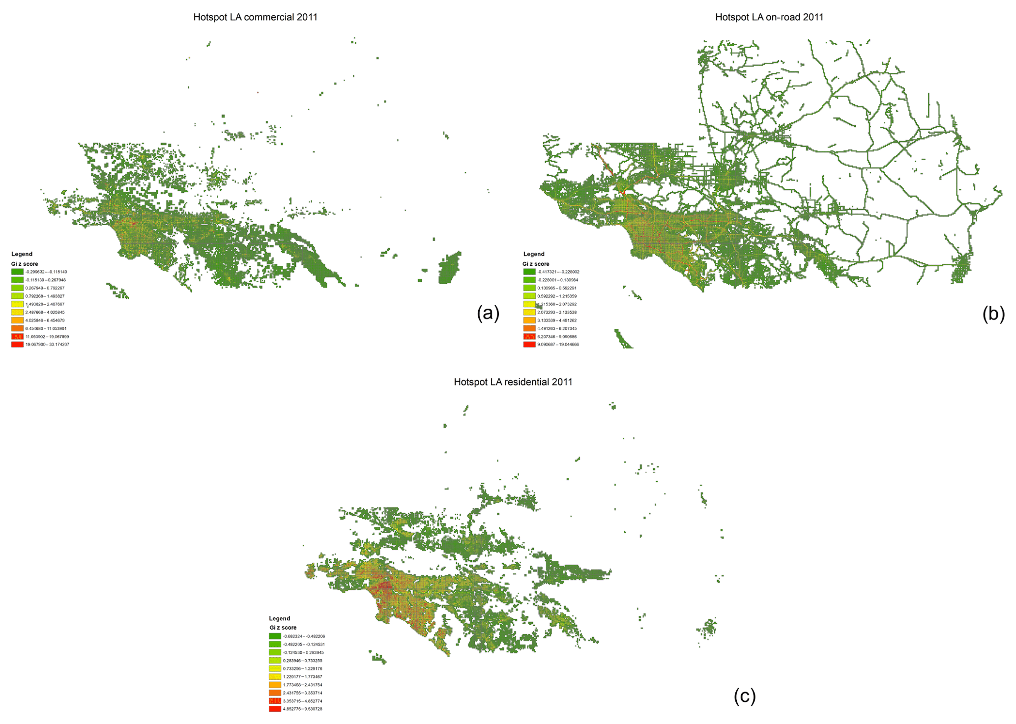
Figure 13The Getis–Ord Gi z score for Hestia-LA FFCO2 emissions across three sectors: (a) commercial, (b) on-road, and (c) residential.
There are very few estimates that can serve as an assessment of the accuracy of the Hestia FFCO2 emissions, as few inventory efforts have been accomplished at the sub-state spatial scale in the United States. However, the Southern California Association of Governments (SCAG) has completed a regional greenhouse gas emissions inventory for a base year period of 1990–2009 with projections out to the year 2035 (Kimberly S. Clark and Christine Fernandez, Southern California Association of personal communication, 2012). The SCAG inventory reflects two components that make a comparison to the Hestia-LA FFCO2 emissions data product imperfect. First, the domain considered in the SCAG inventory includes Imperial county, a county not included in the Hestia-LA domain. However, Imperial county is estimated to be less than a few percent of the SCAG domain total. For example, Imperial county on-road VMT is 1.9 % of the SCAG domain total. The Imperial county retail sales of electricity is 1.1 % of the SCAG domain total. The other distinction is that the SCAG inventory reports total GHGs, inclusive of both methane (CH4) and nitrous oxide (N2O). However, in the sectors and activities used for comparing the SCAG inventory to the Hestia-LA FFCO2 emissions data product, both CH4 and N2O are negligibly small. Hence, small differences (<5 %) could be due to these categorical discrepancies. We use only the reported Scope 1 emissions which were based on the approach adopted by CARB based on guidelines from the Intergovernmental Panel on Climate Change (CARB, 2010).
Figure 14 shows a 2010 comparison between the two estimates using the comparable sector divisions. The Hestia-LA FFCO2 emissions estimate is 10.7 % larger than the SCAG estimate, 95 % of the difference (4.46 MtC yr−1) owing to the larger industrial and electricity production FFCO2 emissions in the Hestia estimate. We have included the non-road sector in the on-road category as the SCAG inventory did not explicitly include a non-road sector. SCAG documentation suggests that the non-road sector is included in the forecasts for the residential, commercial, and industrial sectors (Kimberly S. Clark and Christine Fernandez, Southern California Association of Governments, personal communication, 2012, Parcel Data GIS shapefiles p. C-10), but further details on the base year estimates could not be found and no mention is made in the report where these sectors are described. If the Hestia non-road estimate (1.56 MtC yr−1) was not allocated to the on-road sector but distributed to the residential, commercial, and industrial sectors it would exacerbate the difference in the on-road, commercial, and industrial sectors.
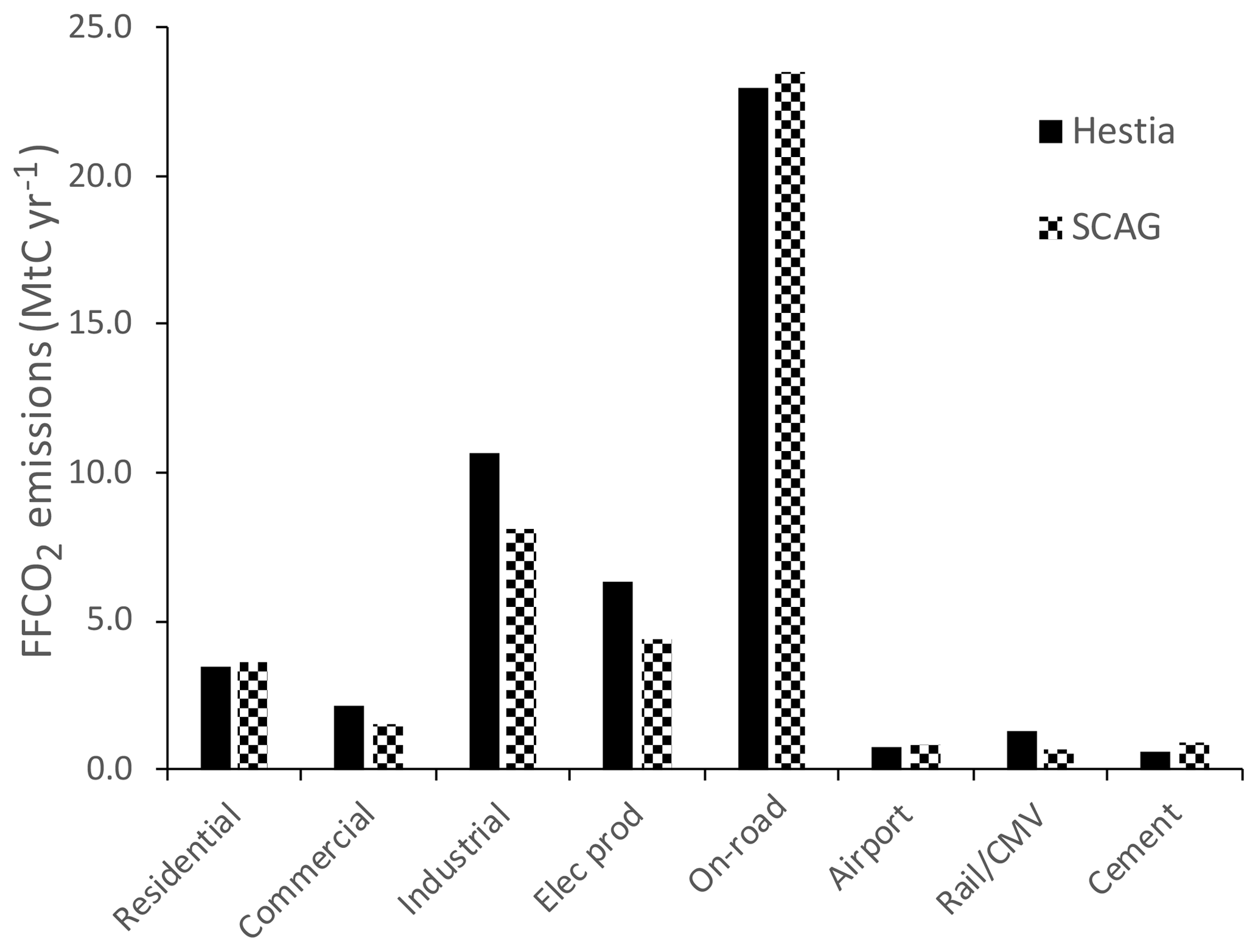
Figure 14Comparison of sector-specific FFCO2 emissions for the year 2010 between the Hestia-LA and SCAG estimates. Units: MtC yr−1.
The California Energy Commission archives energy consumption data for both natural gas and electricity (http://ecdms.energy.ca.gov/, last acces: 12 August 2019). The data are archived as specific to the residential sector and the nonresidential sector. Because of ambiguities regarding the nonresidential sector definition, we compare the reported values by county for the residential only (Table 6). Good agreement for natural gas FFCO2 emissions is achieved for the Los Angeles megacity as a whole (<1 %) with some variation at the scale of the individual counties. Agreement with the CEC estimate is better than that found for the comparison with the SCAG inventory (Hestia being 3.1 % lower than the SCAG residential NG FFCO2 estimate).
Average hourly variations in FFCO2 emissions are sensitive to both the sector and spatial location. Figure 15 presents annual mean diurnal patterns specified by county and sector (the railroad or cement sectors were constructed with no diurnal cycle and hence are not shown). As noted previously, Los Angeles county shows the greatest emissions overall, particularly for the commercial marine vessel sector where the port of Los Angeles dominates. The commercial, residential, on-road, and CMV sectors exhibit two maxima, one in the morning (∼05:00–10:00 local time) and another in the afternoon–evening. In the commercial sector, this afternoon–evening maximum occurs later in this time period centered on 21:00 local time, coinciding with retail closing schedules. The maximum CMV emissions are shifted by roughly 2 h earlier in the day for both the morning and afternoon–evening peaks. The afternoon–evening maximum for the on-road sector shows an afternoon–evening maximum that is of longer duration than that in the morning, with emissions gradually rising after the midpoint of the day, local time. In addition to large daily variations, the on-road sector contains a significant weekly temporal pattern with emissions largest on Monday and smallest on Saturday (Fig. 16).
Diurnal patterns in on-road and airport FFCO2 emissions have a single maximum at the middle of the day but broadly extending across all daylight hours. In the case of the non-road emissions, this is simply a reflection of the EPA temporal surrogate applied. In the case of the airport FFCO2 emissions, the time structure reflects the reported air traffic volume at the major airports in the LA megacity. Finally, the industrial and electricity production sectors maintain relatively constant emissions across the entire 24 h. In the case of the industrial sector, this reflects the integration of industry-specific EPA temporal surrogates within a given county. For the electricity production sector, the time structure is primarily driven by the stack-monitored emissions and shows slightly greater emissions in the evening hours compared to all other hours.
Table 6Residential natural gas FFCO2 emissions in the five Hestia-LA domain counties for the year 2011 compared to estimates from the California Energy Commission (CEC). Units: MtC yr−1.

The diurnal patterns are consistent across all five counties with the exception of the commercial sector where there are small differences in the maximum point of the morning emissions in San Bernardino and Ventura counties compared to the other LA megacity counties.
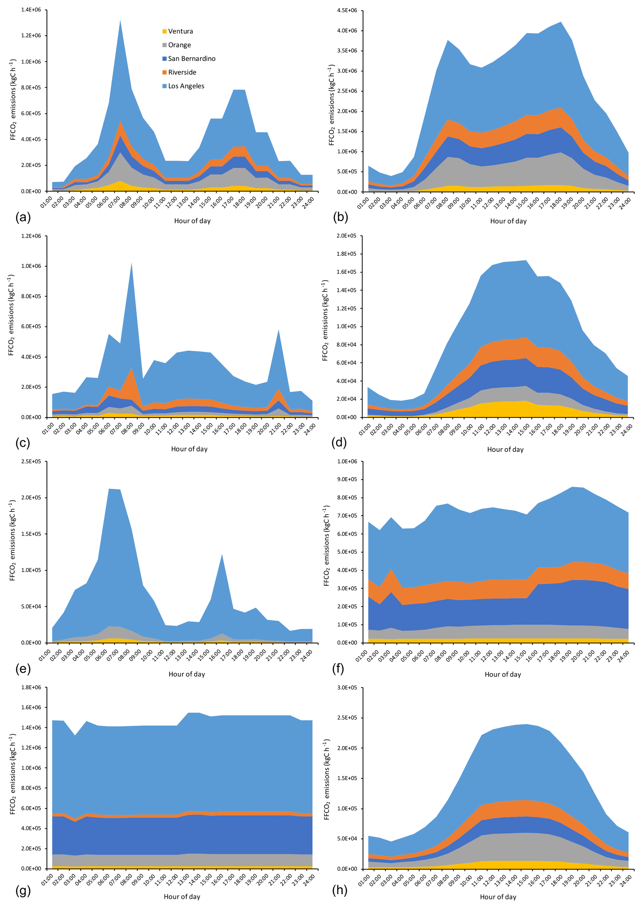
Figure 15Average daily FFCO2 emissions in the Hestia-LA v2.5 data product for five counties across eight sectors: (a) residential, (b) on-road, (c) commercial, (d) airport, (e) commercial marine vessel, (f) electricity production, (g) industrial, and (h) non-road. Note the different scale ranges on each plot. Units: kgC h−1.
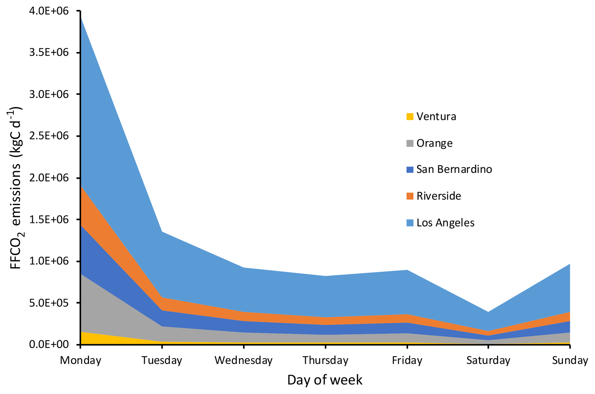
Figure 16Average weekly on-road FFCO2 emissions from the Hestia-LA v2.5 data product for five counties. Units: kgC d−1.
The first Hestia urban FFCO2 emissions data product was produced for the Indianapolis domain (Gurney et al., 2012). As an outcome of the Hestia effort, a large multifaceted effort, the Indianapolis Flux Experiment (INFLUX), emerged (Whetstone, 2018; Davis et al., 2017). INFLUX aims to advance quantification and associated uncertainties of urban CO2 and CH4 emissions by integrating a high-resolution bottom-up emission data product, such as Hestia, with atmospheric concentration measurements (Turnbull et al., 2015; Miles et al., 2017; Richardson et al., 2017), flux measurements (Cambaliza et al., 2014, 2015; Heimburger et al., 2017), and atmospheric inverse modeling. In addition to its use as a key constraint in the INFLUX atmospheric inverse estimation (Lauvaux et al., 2016), Hestia has been informed by atmospheric observations making it useable as a stand-alone high-resolution flux estimate offering a detailed space-time understanding of urban emissions. Begun in the late 2000s, INFLUX has explored many aspects of the individual elements of a scientifically driven urban flux assessment (e.g., Wu et al., 2018), in addition to demonstrating potential reconciliation between Hestia and the atmospheric measurements (Gurney et al., 2017; Turnbull et al., 2015). Similar efforts are ongoing in the Salt Lake City (Mitchell et al., 2018; Lin et al., 2018) and Baltimore (Martin et al., 2018) domains with a different arrangement of atmospheric monitoring and modeling. As with INFLUX, a Hestia FFCO2 emissions data product was produced in each domain (Patarasuk et al., 2016; Gurney et al., 2018).
The Hestia Los Angeles megacity effort was developed under the Megacities Carbon Project framework (https://megacities.jpl.nasa.gov/portal/, last access: 12 August 2019). It was designed to serve the Megacities Carbon Project in a similar capacity to its role in INFLUX. The Hestia-LA results are unique in that it is the first high-resolution spatiotemporally explicit inventory of FFCO2 emissions centered over a megacity. Presented here at the 1 km2 spatial and hourly temporal resolution, the emissions can be represented at finer spatial scales down to the individual building, though with higher uncertainty. While policy emphasis in California thus far has been focused on CH4 emissions (Carranza et al., 2018; Wong et al., 2016; Verhulst et al., 2017; Hopkins et al., 2016), work is ongoing to use the extensive atmospheric CO2 observing capacity in the Los Angeles domain (e.g., Newman et al., 2016; Wong et al., 2015; Wunch et al., 2009) within an atmospheric CO2 inversion. This will offer an important evaluation of the Hestia-LA emissions for which limited independent evaluation is currently available.
The potential of the Hestia-LA FFCO2 emissions to enable or assist with policymaking in the city, county, or metropolitan planning domain of the overall Southern California area is considerable. The traditional urban inventory approach, such as that accomplished by many cities as part of their climate action plans, are whole-city accounts, often specific to sector, that follow one of a few inventory protocols. Given the challenges of data acquisition and the idiosyncrasies of protocol choice and needs, the traditional urban inventories are difficult to compare across cities and hence aggregate reliably in a metropolitan domain such as the LA megacity. Importantly, without explicit space and time emissions information, they are difficult to calibrate with atmospheric measurements and hence evaluate against this important scientific constraint. The Hestia-LA FFCO2 emissions approach attempts to overcome these limitations to traditional inventory work. By quantifying emissions at the scale of individual buildings and road segments, with process detail such as the sector, fuel, and combustion technology, Hestia results can be organized according to most of the protocols in use by cities. This explicit space and time detail also allows for calibration to atmospheric measurements, for which emission location and time structure is essential.
The state of California continues to lead the nation in climate policy with numerous legislative and executive orders outlining both general reduction goals and specific policy instruments. The California Global Warming Solutions Act (Assembly Bill 32) passed in 2006, specifies a statewide reduction in greenhouse gas emissions to 1990 levels by the year 2020 (https://www.arb.ca.gov/cc/ab32/ab32.htm, last access: 12 August 2019). Furthermore, the bill requires reporting and verification of reductions in order to demonstrate compliance. Executive order B-30-15 and Senate Bill SB 32 have built on this with an aim to reduce emissions 40 % below 1990 levels by 2030 and 80 % below 1990 levels by 2050, respectively (https://www.ca.gov/archive/gov39/2015/04/29/news18938/, last access: 12 August 2019; https://leginfo.legislature.ca.gov/faces/billTextClient.xhtml?bill_id=201520160SB32, last access: 12 August 2019). Ultimately, much of the specific action needed to meet these goals will rest upon local governments and authorities. Given that 87 % of the state population resides in urban areas and nearly half of state population resides in the Los Angeles megacity, the cities and counties that comprise the Los Angeles metropolitan area have a central role to play in achieving the statewide climate change policy goals. The city of Los Angeles, the largest individual city in the metro region, has specified goals consistent with the state commitments, expecting to reduce greenhouse gas emissions to 35 % below 1990 levels by the year 2030 (https://coolcalifornia.arb.ca.gov/story/city-of-los-angeles, last access: 12 August 2019). To meet these reduction goals, policy actions will become increasingly difficult to achieve at no or low cost and economic efficiency will become central to making policy choices. The most important attribute of the Hestia-LA approach, therefore, is the potential it offers for targeting urban CO2 reduction policy more efficiently. As shown in Figs. 12 and 13, FFCO2 emissions are highly variable in space and typically cluster in concentrated areas. In choosing specific policy approaches and instruments, this offers Los Angeles policymakers the ability to target specific neighborhoods, road segments, or commercial hubs, where policies will achieve the greatest reduction for resources expended. This rests on the argument that specificity leads to efficiency. As all cities, including those in the Los Angeles megacity, move towards those aspects of carbon emission reductions that are not part of the “low-hanging fruit” policy instruments, competition for limited resources and policy justification will increase. Having information that targets the most efficient and effective emission reduction investments, established by independent rigorous scientific information, will be at a premium. For example, if a small proportion of the commercial sector buildings in the LA megacity account for a large proportion of the FFCO2 emissions, knowing the location of these buildings and targeting energy efficiency programs to those buildings, may offer the most economically efficient route to emissions reductions in the commercial sector. A similar argument can be made in the on-road sector due to the clustering of large on-road emitting grid cells and specific road-class attributes (see Rao et al., 2017).
A number of caveats are worth mentioning in association with the Hestia-LA v2.5 FFCO2 emissions results. With Vulcan v3.0 as the starting point for the quantification in Hestia, errors in Vulcan will be passed to Hestia, with a few exceptions. Of particular note are the industrial sector and, more specifically, refining operations which have limited emissions reporting. These remain difficult to quantify due to the range of CO emission factors representing many of the combustion processes undertaken at these large and complex facilities. The uncertainty estimation described remains limited and there are additional sources of uncertainty that must be quantified such as categorical errors (e.g., misspecification of fuel category or road class), errors in spatial accuracy and spatial error correlation. Quantifying these contributions to the overall uncertainty presented here remain a task for future work.
The Hestia-LA v2.5 emissions data product can be downloaded from the data repository at the National Institute of Standards and Technology (https://doi.org/10.18434/T4/1502503, Gurney et al., 2019) and is distributed under Creative Commons Attribution 4.0 International (CC-BY 4.0, https://creativecommons.org/licenses/by-nc-sa/4.0/, last access: 12 August 2019). The Hestia-LA v2.5 FFCO2 emissions data product is provided as annual and hourly (local and UTC versions) 1 km × 1 km NetCDF file formats, one file for each of the 6 years (2010–2015). The hourly files are approximately 2.9 GB each. The annual files are 0.34 GB each.
Attempts will be made to update the Hestia-LA FFCO2 emissions on a roughly bi-annual basis, depending upon support, the availability of updates to the Vulcan FFCO2 emissions data product, and updates to the additional data sources described in this study.
The Hestia Project quantifies urban fossil fuel CO2 emissions at high space- and time-resolution with application to both scientific and policy arenas. We present here the Hestia-LA version 2.5 FFCO2 emissions data product, which represents hourly, 1 km2, sector-specific emissions for the five counties of the Los Angeles metropolitan area for the 2010 to 2015 time period. The methodology relies on the results of the Vulcan Project (version 3.0) further enhancing and distributing emissions to the scale of individual buildings and road segments with local data sources acquired from local government agencies. Each sector is quantified using data sources and spatial and temporal distribution approaches distinct to the sector characteristics. The results offer a detailed view of FFCO2 emissions across the LA megacity and point to the extreme spatial variance of emissions. For example, 10 % of the 1 km2 emitting grid cells account for 93.6 %, 73.4 %, 66.2 %, and 45.3 % of the emissions in the industrial, on-road, commercial, and residential sectors, respectively. We find that the LA megacity emitted 48.06±5.3 MtC yr−1 in the year 2011, dominated by Los Angeles county (26.42±2.9 MtC yr−1) and from a sector-specific viewpoint, dominated by the on-road sector (20.81±2.3 MtC yr−1). Hestia FFCO2 emissions are 10.7 % larger than the inventory estimate generated by the local metropolitan planning agency, a difference that is driven by the industrial and electricity production sectors. Good agreement is found (<1 %) when comparing residential natural gas FFCO2 emissions to utility-based reporting at the county spatial scale. The largest temporal variations are found in the diurnal cycle with the residential, commercial, on-road, and commercial marine vessel emissions showing two maxima, one in the morning and a second in the afternoon–evening. Airport and non-road emissions, by contrast show broad maxima across the daylight hours. Finally, the industrial and electricity production sectors show little diurnal variation across 24 h. The on-road sector also exhibits variation in the weekly distribution of emissions with maximum FFCO2 emissions on Monday and minimum emissions on Saturday.
The Hestia-LA v2.5 FFCO2 emissions data product offers the scientific and policymaking communities unprecedented spatially and temporally resolved information on FFCO2 emission sources in the Los Angeles megacity. As part of the Megacities Carbon Project, future work includes incorporation into atmospheric CO2 inversion research to further evaluate the Hestia-LA data product and improve estimation. Policymakers can use the Hestia-LA results to better understand FFCO2 emissions at the human scale, offering the potential for improved targeting of FFCO2 reduction policy instruments. Finally, urban researchers can use Hestia-LA to explore a number of important urban science questions such as how emissions intersect with other urban sociodemographic variables such as income, education, housing size, or vehicle ownership.
The Hestia-LA data product is publicly available and will be updated with future years as data becomes available.
KRG conceived of the content, performed portions of the analysis, and wrote the paper. RP, JL, and PR contributed data product development and analysis. YS and DO'K contributed to development and analysis. JW, RD, AE, and CM contributed conceptual content.
The authors declare that they have no conflict of interest.
We thank Lan Nguyan from the City of Los Angeles, Andy Alexis from the California Air Resources Board, and Cheol-Ho Lee at the Southern California Association of Governments for guidance on data use.
This research was made possible through support from the National Aeronautics and Space Administration Carbon Monitoring System program, the Understanding User Needs for Carbon Information project (subcontract no. 1491755), the National Aeronautics and Space Administration (grant no. NNX14AJ20G), the National Institute of Standards and Technology (grant nos. 70NANB14H321 and 70NANB16H264), the Jet Propulsion Laboratory’s Strategic University Research Partnership program, and the Trust for Public Land.
This paper was edited by Scott Stevens and reviewed by two anonymous referees.
Andrew, R. M.: Global CO2 emissions from cement production, Earth Syst. Sci. Data, 10, 195–217, https://doi.org/10.5194/essd-10-195-2018, 2018.
Bellassen, V., Stephan, N., Afriat, M., Alberola, E., Barker, A., Chang, J. P., and Shishlov, I.: Monitoring, reporting and verifying emissions in the climate economy, Nat. Clim. Change, 5, 319–328, https://doi.org/10.1038/nclimate2544, 2015.
Bulkeley, H.: Cities and the Governing of Climate Change, SSRN (Vol. 35), Annual Reviews, https://doi.org/10.1146/annurev-environ-072809-101747, 2010.
Bréon, F. M., Broquet, G., Puygrenier, V., Chevallier, F., Xueref-Remy, I., Ramonet, M., Dieudonné, E., Lopez, M., Schmidt, M., Perrussel, O., and Ciais, P.: An attempt at estimating Paris area CO2 emissions from atmospheric concentration measurements, Atmos. Chem. Phys., 15, 1707–1724, https://doi.org/10.5194/acp-15-1707-2015, 2015.
Cambaliza, M. O. L., Shepson, P. B., Caulton, D. R., Stirm, B., Samarov, D., Gurney, K. R., Turnbull, J., Davis, K. J., Possolo, A., Karion, A., Sweeney, C., Moser, B., Hendricks, A., Lauvaux, T., Mays, K., Whetstone, J., Huang, J., Razlivanov, I., Miles, N. L., and Richardson, S. J.: Assessment of uncertainties of an aircraft-based mass balance approach for quantifying urban greenhouse gas emissions, Atmos. Chem. Phys., 14, 9029–9050, https://doi.org/10.5194/acp-14-9029-2014, 2014.
Cambaliza, M. O. L., Shepson, P. B., Bogner, J., Caulton, D. R., Stirm, B., Sweeney, C., Montzka, S. A., Gurney, K. R., Spokas, K., Salmon, O. E., Lavoie, T. N., Hendricks, A., Mays, K., Turnbull, J., Miller, B. R., Lauvaux, T., Davis, K., Karion, A., Moser, B., Miller, C., Obermeyer, C., Whetstone, J., Prasad, K., Miles, N., and Richardson, S.: Quantification and source apportionment of the methane emission flux from the city of Indianapolis, Elementa Science of the Anthropocene, 3, 3:000037, https://doi.org/10.12952/journal.elementa.000037, 2015.
California Air Resources Board (CARB): Documentation of California's Greenhouse Gas Inventory, June 2010, available at: https://ww3.arb.ca.gov/cc/inventory/data/data.htm/ghg_inventory_00-17_method_update_document.pdf (last access: 12 August 2019), 2010.
California Air Resources Board (CARB): EMFAC2014 Volume I – User's Guide, v1.0.7, 30 April 2014, California Environmental Protection Agency Air Resources Board, Mobile Source Analysis Branch, Air Quality Planning & Science Division, EMFAC data available at: https://www.arb.ca.gov/emfac/2014/ (last access: 12 August 2019), 2014.
California Energy Commission (CEC): California Commercial End-Use Survey, CEC-400-2006-005, available at: http://www.energy.ca.gov/ceus/2006_enduse.html (last access: 1 August 2018), 2006.
Carranza, V., Rafiq, T., Frausto-Vicencio, I., Hopkins, F. M., Verhulst, K. R., Rao, P., Duren, R. M., and Miller, C. E.: Vista-LA: Mapping methane-emitting infrastructure in the Los Angeles megacity, Earth Syst. Sci. Data, 10, 653–676, https://doi.org/10.5194/essd-10-653-2018, 2018.
Chavez, A. and Ramaswami, A.: Progress toward low carbon cities: Approaches for transboundary GHG emissions' footprinting, Carbon Manag., 2, 471–482, https://doi.org/10.4155/cmt.11.38, 2011.
Christen, A.: Atmospheric measurement techniques to quantify greenhouse gas emissions from cities, Urban Climate, 10, 241–260, https://doi.org/10.1016/j.uclim.2014.04.006, 2014.
Christen, A.: Atmospheric measurement techniques to quantify greenhouse gas emissions from cities, Urban Climate, 10, 241–260. https://doi.org/10.1016/j.uclim.2014.04.006, 2014.
Clark, S. S. and Chester, M. V.: A hybrid approach for assessing the multi-scale impacts of urban resource use: Transportation in Phoenix, Arizona, J. Ind. Ecol., 21, 136–150, https://doi.org/10.1111/jiec.12422, 2017.
Commercial Building Energy Consumption Survey (CBECS): 2012 CBECS microdata files and information, U.S. Energy Information Administration, Data available at:: https://www.eia.gov/consumption/commercial/data/2012/index.php?view=microdata (last access: 1 August 2018), 2016.
Davis, K. J., Deng, A., Lauvaux, T., Miles, N. L., Richardson, S. J., Sarmiento, D., Gurney, K. R., Hardesty, R. M., Brewer, A., Shepson, P. B., Cambaliza, M. O., Sweeney, C., Turnbull, J., Whetstone, J., and Karion, A.: The Indianapolis Flux Experiment (INFLUX): A test-bed for developing anthropogenic greenhouse gas measurements, Elementa Science of the Anthropocene, 5, 21, https://doi.org/10.1525/elementa.188, 2017.
Department of Energy/Energy Information Administration (DOE/EIA): State Energy Consumption Estimates 1960 through 2016, DOE/EIA-0214(2016), Washington DC, June 2018.
Department of Energy/Energy Information Administration (DOE/EIA): Electric Power Monthly March 2003 Energy Information Administration, Office of Coal, Nuclear, and Alternate Fuels, US Department of Energy, Washington DC, 20585, DOE/EIA form 923 reporting data available at: http://www.eia.gov/electricity/data/eia923 (last access: 27 July 2018), 2003.
Djuricin, S., Pataki, D. E., and Xu, X.: A comparison of tracer methods for quantifying CO2 sources in an urban region, J. Geophys. Res., 115, D11303, https://doi.org/10.1029/2009jd012236, 2010.
Duren, R. M. and Miller, C. E.: Towards robust global greenhouse gas monitoring, Greenhouse Gas Measurement and Management, 1, 80–84, https://doi.org/10.1080/20430779.2011.579356, 2011.
Erickson, P. and Lazarus, M.: Revisiting community-scale greenhouse gas inventories, Environ. Sci. Technol., 46, 4693–4694, https://doi.org/10.1021/es301366b, 2012.
Erickson, P. and Lazarus, M.: Global emissions: New oil investments boost carbon lock-in, Nature, 526, 43–43, 2015.
Federal Aviation Administration (FAA): OPSNET Manual, available at: http://aspmhelp.faa.gov/index.php/OPSNET_Manual, data available at: https://aspm.faa.gov/opsnet/sys/main.asp, last access: 1 August 2018a.
Federal Aviation Administration (FAA): ETMSC Manual, available at: http://aspmhelp.faa.gov/index.php/ETMSC_Manual, data available at: https://aspm.faa.gov/tfms/sys/main.asp, last access: 1 August 2018b.
Federal Emergency Management Agency (FEMA): HAZUS database, available at: https://www.fema.gov/summary-databases-hazus-multi-hazard (last access: 1 August 2018), 2017.
Feng, S., Lauvaux, T., Newman, S., Rao, P., Ahmadov, R., Deng, A., Díaz-Isaac, L. I., Duren, R. M., Fischer, M. L., Gerbig, C., Gurney, K. R., Huang, J., Jeong, S., Li, Z., Miller, C. E., O'Keeffe, D., Patarasuk, R., Sander, S. P., Song, Y., Wong, K. W., and Yung, Y. L.: Los Angeles megacity: a high-resolution land–atmosphere modelling system for urban CO2 emissions, Atmos. Chem. Phys., 16, 9019–9045, https://doi.org/10.5194/acp-16-9019-2016, 2016.
Fong, W. K., Sotos, M., Doust, M., Schultz, S., Marques, A., and Deng-Beck, C.: Global Protocol for Community-Scale Greenhouse Gas Emissions Inventories: An Accounting and Reporting Standard for Cities, WRI/C40/ICLEI, 2014.
Font, A., Grimmond, C. S. B., Kotthaus, S., Morguí, J. A., Stockdale, C., O'Connor, E., Priestman, M., and Barratt, B.: Daytime CO2 urban surface fluxes from airborne measurements, eddy-covariance observations and emissions inventory in Greater London, Environ. Pollut., 196, 98–106, https://doi.org/10.1016/j.envpol.2014.10.001, 2015.
Getis, A. and Ord, J. K.:. The analysis of spatial association by use of distance statistics, Geogr. Anal., 24, 189–206, 1992.
Grimmond, C. S. B., King, T. S., Cropley, F. D., Nowak, D. J., and Souch, C.: Local-scale fluxes of carbon dioxide in urban environments: Methodological challenges and results from Chicago, Environ. Pollut., 116 (Suppl. 1), S243–S254, https://doi.org/10.1016/S0269-7491(01)00256-1, 2002.
Güneralp, B., Zhou, Y., Ürge-Vorsatz, D., Gupta, M., Yu, S., Patel, P. L., and Seto, K. C.: Global scenarios of urban density and its impacts on building energy use through 2050, P. Natl. Acad. Sci. USA, 114, 8945–8950, https://doi.org/10.1073/pnas.1606035114, 2017.
Gurney, K. R., Mendoza, D., Zhou, Y., Fischer, M., de la Rue du Can, S., Geethakumar, S., and Miller, C.: The Vulcan Project: High resolution fossil fuel combustion CO2 emissions fluxes for the United States, Environ. Sci. Technol., 43, 5535–5541, https://doi.org/10.1021/es900806c, 2009.
Gurney, K. R., Razlivanov, I., Song, Y., Zhou, Y., Benes, B., Abdul-Massih, M.: Quantification of fossil fuel CO2 on the building/street scale for a large US city, Environ. Sci. Technol., 46, 12194–12202, https://doi.org/10.1021/es3011282, 2012.
Gurney, K. R., Huang, J., and Coltin, K.: Comment on quick, J. C. (2014) carbon dioxide emission tallies for 210 US coal-fired power plants: a comparison of two accounting methods, J. Air Waste Manage., 64, 73–79, J. Air Waste Manage., 64, 1215–1217, 2014.
Gurney, K. R., Romero-Lankao, P., Seto, K., Kennedy, C., Grimm, N., Ehleringer, J., Marcotullio, P., Pincetl, S., Feddema, J. J., Hughes, S., Chester, M. V., Hutyra, L., Sperling, J., and Runfola, D.: Climate change: Track urban emissions on a human scale, Nature (Comment), 525, 179–181, https://doi.org/10.1038/525179a, 2015.
Gurney, K. R., Huang, J., and Coltin, K.: Bias present in US federal agency power plant CO2 emissions data and implications for the US clean power plan, Environ. Res. Lett., 11, 064005, https://doi.org/10.1088/1748-9326/11/6/064005, 2016.
Gurney, K. R., Liang, J., Patarasuk, R., O'Keeffe, D., Huang, J., Hutchins, M., Lauvaux, T., Turnbull, J. C., and Shepson, P. B.: Reconciling the differences between a bottom-up and inverse-estimated FFCO2 emissions estimate in a large U.S. urban area, Elementa Science of the Anthropocene, 5, 44, https://doi.org/10.1525/elementa.137, 2017.
Gurney, K. R., Liang, J., O'Keeffe, D. O., Patarasuk, R., Hutchins, M., Huang, J., Rao, P., and Song, Y.: Comparison of Global Downscaled Versus Bottom-Up Fossil Fuel CO2 Emissions at the Urban Scale in Four US Urban Areas, J. Geophys. Res.-Atmos., 124, 2823–2840, https://doi.org/10.1029/2018JD028859, 2018.
Gurney, K. R., Liang, J., O'Keeffe, D., Huang, J., Song, Y., Rao, P., Wong, T. M.: Hestia Fossil Fuel Carbon Dioxide (FFCO2) Data Product – Los Angeles Basin, Version 2.5, 1 km grid, https://doi.org/10.18434/T4/1502503, 2019.
Heimburger, A. M. F., Harvey, R. M., Shepson, P. B., Stirm, B. H., Gore, C., Turnbull, J., Cambaliza, M. O. L, Salmon, O. E., Kerlo, A.-E. M., Lavoie, T. N., Davis, K. J., Lauvaux, T., Karion, A., Sweeney, C., Brewer, W. A., Hardesty, R. M., and Gurney, K. R.: Assessing the optimized precision of the aircraft mass balance method for measurement of urban greenhouse gas emission rates through averaging, Elementa Science of the Anthropocene, 5, 26, https://doi.org/10.1525/elementa.134, 2017.
Hirsch, J. and Associates: Energy Simulation Training for Design & Construction Professionals, available at: http://doe2.com/download/equest/eQuestTrainingWorkbook.pdf, eQuest model download available at: http://www.doe2.com/eQuest/ (last access: 1 August 2018), 2004.
Homer, C. G., Dewitz, J. A., Yang, L., Jin, S., Danielson, P., Xian, G., Coulston, J., Herold, N. D., Wickham, J. D., and Megown, K.: Completion of the 2011 National Land Cover Database for the conterminous United States-Representing a decade of land cover change information, Photogramm. Eng. Rem. S., 81, 345–354, 2015.
Hopkins, F. M., Kort, E. A., Bush, S. E., Ehleringer, J., Lai, C., Blake, D., and Randerson, J. T.: Spatial patterns and source attribution of urban methane in the Los Angeles Megacity, J. Geophys. Res.-Atmos., 121, 2490–2507, https://doi.org/10.1002/2015JD024429, 2016.
Hsu, A., Moffat, A. S., Weinfurter, A. J., and Schwartz, J. D.:. Towards a new climate diplomacy, Nat. Clim. Change, 5, 501–503, https://doi.org/10.1038/nclimate2594, 2015.
Hsu, A., Weinfurter, A. J., and Xu, K.: Aligning subnational climate actions for the new post-Paris climate regime, Climatic Change, 142, 419–432, https://doi.org/10.1007/s10584-017-1957-5, 2017.
Hutyra, L. R., Duren, R., Gurney, K. R., Grimm, N., Kort, E. A., Larson, E., and Shrestha, G.: Urbanization and the carbon cycle: Current capabilities and research outlook from the natural sciences perspective, Earth's Future, 2, 473–495, https://doi.org/10.1002/2014ef000255, 2014.
IPCC: Guidelines for National Greenhouse Gas Inventories, Directrices para los inventarios nacionales GEI, p. 12, available at: http://www.ipcc-nggip.iges.or.jp/public/2006gl/index.html (last access: 12 August 2019), 2006.
IPCC: Climate Change 2013: The Physical Science Basis. Contribution of Working Group I to the Fifth Assessment Report of the Intergovernmental Panel on Climate Change, edited by: Stocker, T. F., Qin, D., Plattner, G.-K., Tignor, M., Allen, S. K., Boschung, J., Nauels, A., Xia, Y., Bex, V., and Midgley, P. M., Cambridge University Press, Cambridge, United Kingdom and New York, NY, USA, 1535 pp., 2013.
Jones, C. and Kammen, D. M.: Spatial distribution of U.S. household carbon footprints reveals suburbanization undermines greenhouse gas benefits of urban population density, Environ. Sci. Technol., 48, 895–902, https://doi.org/10.1021/es4034364, 2014.
Kort, E. A., Frankenberg, C., Miller, C. E., and Oda, T.: Space-based observations of megacity carbon dioxide, Geophys. Res. Lett., 39, L17806, https://doi.org/10.1029/2012gl052738, 2012.
Lauvaux, T., Miles, N. L., Richardson, S. J., Deng, A., Stauffer, D., Davis, K. J., Jacobson, G., Rella, C., Calonder, G.-P., and DeCola, P. L.: Urban emissions of CO2 from Davos, Switzerland: the first real-time monitoring system using an atmospheric inversion technique, J. Appl. Meteorol. Clim., 52, 2654–2668, https://doi.org/10.1175/JAMC-D-13-038.1, 2013.
Lauvaux, T., Miles, N. L., Deng, A., Richardson, S. J., Cambaliza, M. O., Davis, K. J., Gaudet, B., Gurney, K. R., Huang, J., O'Keefe, D., Song, Y., Karion, A., Oda, T., Patarasuk, R., Razlivanov, I., Sarmiento, D., Shepson, P., Sweeney, C., Turnbull, J., and Wu, K.: High-resolution atmospheric inversion of urban CO2 emissions during the dormant season of the Indianapolis Flux Experiment (INFLUX), J. Geophys. Res.-Atmos., 121, 5213–5236, https://doi.org/10.1002/2015JD024473, 2016.
Le Quéré, C., Andrew, R. M., Friedlingstein, P., Sitch, S., Pongratz, J., Manning, A. C., Korsbakken, J. I., Peters, G. P., Canadell, J. G., Jackson, R. B., Boden, T. A., Tans, P. P., Andrews, O. D., Arora, V. K., Bakker, D. C. E., Barbero, L., Becker, M., Betts, R. A., Bopp, L., Chevallier, F., Chini, L. P., Ciais, P., Cosca, C. E., Cross, J., Currie, K., Gasser, T., Harris, I., Hauck, J., Haverd, V., Houghton, R. A., Hunt, C. W., Hurtt, G., Ilyina, T., Jain, A. K., Kato, E., Kautz, M., Keeling, R. F., Klein Goldewijk, K., Körtzinger, A., Landschützer, P., Lefèvre, N., Lenton, A., Lienert, S., Lima, I., Lombardozzi, D., Metzl, N., Millero, F., Monteiro, P. M. S., Munro, D. R., Nabel, J. E. M. S., Nakaoka, S.-I., Nojiri, Y., Padin, X. A., Peregon, A., Pfeil, B., Pierrot, D., Poulter, B., Rehder, G., Reimer, J., Rödenbeck, C., Schwinger, J., Séférian, R., Skjelvan, I., Stocker, B. D., Tian, H., Tilbrook, B., Tubiello, F. N., van der Laan-Luijkx, I. T., van der Werf, G. R., van Heuven, S., Viovy, N., Vuichard, N., Walker, A. P., Watson, A. J., Wiltshire, A. J., Zaehle, S., and Zhu, D.: Global Carbon Budget 2017, Earth Syst. Sci. Data, 10, 405–448, https://doi.org/10.5194/essd-10-405-2018, 2018.
Lin, J. C., Mitchell, M., Buchert, E., Crosman, E., Mendoza, D., Gurney, K. R., Patasuruk, R., Bowling, D., Pataki, D., Bares, R., Fasoli, B., Catherine, D., Baasandorj, M., Jacques, A., Hoch, S., Horel, J., and Ehleringer, J.: CO2 and carbon emissions from cities: linkages to air quality, socioeconomic activity and stakeholders in the Salt Lake City urban area, B. Am. Meteorol. Soc., 99, 2325–2339. https://doi.org/10.1175/bams-d-17-0037.1, 2018.
Los Angeles County (LAC): Countywide Building Outlines – 2014 Update – Public Domain Release, available at: https://egis3.lacounty.gov/dataportal/2016/11/03/countywide-building-outlines-2014-update-public-domain-release/ (last access: 1 August 2018), 2016.
Manufacturing Energy Consumption Survey (MECS): 2010 MECS Survey Data, U.S. Energy Information Administration, available at: https://www.eia.gov/consumption/manufacturing/data/2010/\#r10 (last access: 1 August 2018), 2010.
Marion, W. and Urban, K.: User's Manual for TMY2s Typical Meteorological Years, National Renewable Energy Laboratory (NREL), available at: http://rredc.nrel.gov/solar/pubs/tmy2/PDFs/tmy2man.pdf (last access: 22 July 2014), 1995.
Martin, C. R., Zeng, N., Karion, A., Mueller, K., Ghosh, S., Lopez-Coto, I., Gurney, K. R., Oda, T., Prasad, K., Liu, Y., Dickerson, R. R., and Whetstone, J.: Investigating Sources of Variability and Error in Simulations of Carbon Dioxide in an Urban Region, Atmos. Environ., 199, 55–69, https://doi.org/10.1016/j.atmosenv.2018.11.013, 2018.
Mays, K. L., Shepson, P. B., Stirm, B. H., Karion, A., Sweeney, C., and Gurney, K. R.: Aircraft-Based Measurements of the Carbon Footprint of Indianapolis, Environ. Sci. Technol., 43, 7816–7823, https://doi.org/10.1021/es901326b, 2009.
McKain, K., Wofsy, S. C., Nehrkorn, T., Eluszkiewicz, J., Ehleringer, J. R., and Stephens, B. B.: Assessment of ground-based atmospheric observations for verification of greenhouse gas emissions from an urban region, P. Natl. Acad. Sci. USA, 109, 8423–8428, https://doi.org/10.1073/pnas.1116645109, 2012.
Menzer, O., Meiring, W., Kyriakidis, P. C., and McFadden, J. P.: Annual sums of carbon dioxide exchange over a heterogeneous urban landscape through machine learning based gap-filling, Atmos. Environ., 101, 312–327, https://doi.org/10.1016/j.atmosenv.2014.11.006, 2015.
Miles, N. L., Richardson, S. J., Lauvaux, T., Davis, K. J., Deng, A., Turnbull, J. C., Sweeney, C., Gurney, K. R., Patarasuk, R., Razlivanov, I., Cambaliza, M. O. L., and Shepson, P. B.: Quantification of urban atmospheric boundary layer greenhouse gas dry mole fraction enhancements: Results from the Indianapolis Flux Experiment (INFLUX), Elementa Science of the Anthropocene, 5, 27, https://doi.org/10.1525/elementa.127, 2017.
Mitchell, L., Lin, J. C., Bowling, D. R., Pataki, D. E., Strong, C., Schauer, A. J., Bares, R., Bush, S. E., Stephens, B. B., Mendoza, D., Mallia, D., Holland, L., Gurney, K. R., and Ehleringer, J. R.: Long-term urban carbon dioxide observations reveal spatial and temporal dynamics related to urban characteristics and growth, P. Natl. Acad. Sci. USA, 115, 2912–2917, https://doi.org/10.1073/pnas.1702393115, 2018.
Mount, D. M. and Arya, S.: ANN: A Library for Approximate Nearest Neighbor Searching, Version 1.1.2, Release Date: 27 January 2010, available at: https://www.cs.umd.edu/~mount/ANN/ (last access: 1 August 2018), 2010.
Newman, S., Xu, X., Gurney, K. R., Hsu, Y. K., Li, K. F., Jiang, X., Keeling, R., Feng, S., O'Keefe, D., Patarasuk, R., Wong, K. W., Rao, P., Fischer, M. L., and Yung, Y. L.: Toward consistency between trends in bottom-up CO2 emissions and top-down atmospheric measurements in the Los Angeles megacity, Atmos. Chem. Phys., 16, 3843–3863, https://doi.org/10.5194/acp-16-3843-2016, 2016.
Patarasuk, R., Gurney, K. R., O'Keeffe, D., Song, Y., Huang, J., Rao, P., Buchert, M., Lin, J. C., Mendoza, D., and Ehleringer, J. R.: Urban high-resolution fossil fuel CO2 emissions quantification and exploration of emission drivers for potential policy applications, Urban Ecosyst., 19, 1013–1039, https://doi.org/10.1007/s11252-016-0553-1, 2016.
Porse, E., Derenski, J., Gustafson, H., Elizabeth, Z., and Pincetl, S.: Structural, geographic, and social factors in urban building energy use: Analysis of aggregated account-level consumption data in a megacity, Energ. Policy, 96, 179–192, https://doi.org/10.1016/j.enpol.2016.06.002, 2016.
Performance Measurement System (PeMS): Data Source, available at: http://www.dot.ca.gov/trafficops/mpr/source.html, last access: 1 August 2018.
Portland Cement Company, Economic Research Department: U.S. and Canadian Portland Cement Industry Plant Information Summary, Portland Cement Association, Skokie, IL, 2006.
Quick, J.: Carbon dioxide emission tallies for 210 US coal-fired power plants: a comparison of two accounting methods, J. Air Waste Manage., 64 73–9, 2014.
Ramaswami, A., Hillman, T., Janson, B., Reiner, M., and Thomas, G.: A demand-centered, hybrid life-cycle methodology for city-scale greenhouse gas inventories, Environ. Sci. Technol., 42, 6455–6461, https://doi.org/10.1021/es702992q, 2008.
Rao, P., Gurney, K. R., Patarasuk, R., Yang, S., Miller, C. E., Duren, R. M., and Eldering, A.: Spatio-temporal variations in on-road CO2 emissions in the Los Angeles Megacity, AIMS Geosci., 3, 239–267, https://doi.org/10.3934/geosci.2017.2.239, 2017.
Ramaswami, A. and Chavez, A.: What metrics best reflect the energy and carbon intensity of cities? Insights from theory and modeling of 20 US cities, Environ. Res. Lett., 8, 3, https://doi.org/10.1088/1748-9326/8/3/035011, 2013.
Residential Energy Consumption Survey (RECS): 2009 RECS Survey Data, U.S. Energy Information Administration, available at: https://www.eia.gov/consumption/residential/data/2009/index.php?view=microdata (last access: 1 August 2018), 2013.
Richardson, S. J., Miles, N. L., Davis, K. J., Lauvaux, T., Martins, D. K., Turnbull, J. C., McKain, K., Sweeney, C., and Cambaliza, M. O. L.: Tower measurement network of in-situ CO2, CH4, and CO in support of the Indianapolis FLUX (INFLUX) Experiment, Elementa Science of the Anthropocene, 5, 59, https://doi.org/10.1525/elementa.140, 2017.
Rosenzweig, C., Solecki, W., Hammer, S. A., and Mehrotra, S.: Cities_lead_the_way_in_climate.PDF, Nature, 7318, p. 909, 2010.
Sargent, M., Barrera, Y., Nehrkorn, T., Hutyra, L. R., Gately, C. K., Mckain, K., Sweeney, C., Hegarty, J., Hardiman, B., Wang, J. A., and Wofsy, S. C.: Anthropogenic and biogenic CO2 fluxes in the Boston urban region, P. Natl. Acad. Sci. USA, 115, E9507–E9507, https://doi.org/10.1073/pnas.1815348115, 2018.
Schwandner, F. M., Gunson, M. R., Miller, C. E., Carn, S. A., Eldering, A., Krings, T., and Podolske, J. R.: Spaceborne detection of localized carbon dioxide sources, Science, 358, eaam5782, https://doi.org/10.1126/science.aam5782, 2017.
Seto, K. C., Guneralp, B., and Hutyra, L. R.: Global forecasts of urban expansion to 2030 and direct impacts on biodiversity and carbon pools, P. Natl. Acad. Sci. USA, 109, 16083–16088, https://doi.org/10.1073/pnas.1211658109, 2012.
Seto, K. C., Davis, S. J., Mitchell, R. B., Stokes, E. C., Unruh, G., Ürge-Vorsatz, D., and Urge-Vorsatz, D.: Carbon Lock-In: Types, Causes, and Policy Implications, Annual Review of Environment and Resources, 41, 425–452, https://doi.org/10.1146/annurev-environ-110615-085934, 2016.
Seto, K. C., Dhakal, S., Bigio, A., Blanco, H., Delgado, G. C., Dewar, D., Huang, L., Inaba, A., Kansal, A., Lwasa, S., McMahon, J., Muller, D. B., Murakami, J., Nagendra, H., and Ramaswami, A.: Human Settlements, Infrastructure and Spatial Planning, in: Climate Change 2014: Mitigation of Climate Change, Contribution of Working Group III to the Fifth Assessment Report of the Intergovernmental Panel on Climate Change, edited by: Edenhofer, O., Pichs-Madruga, R., Sokona, Y., Farahani, E., Kadner, S., Seyboth, K., Adler, A., Baum, I., Brunner, S., Eickemeier, P., Kriemann, B., Savolainen, J., Schlömer, S., von Stechow, C., Zwickel, T., and Minx, J. C., Cambridge University Press, Cambridge, United Kingdom and New York, NY, US, 2014.
Shu, Y., and Lam, S. N.: Spatial disaggregation of carbon dioxide emissions from road traffic based on multiple linear regression model, Atmos. Environ., 45, 634–640, https://doi.org/10.1016/j.atmosenv.2010.10.037, 2011.
Staufer, J., Broquet, G., Bréon, F.-M., Puygrenier, V., Chevallier, F., Xueref-Rémy, I., Dieudonné, E., Lopez, M., Schmidt, M., Ramonet, M., Perrussel, O., Lac, C., Wu, L., and Ciais, P.: The first 1-year-long estimate of the Paris region fossil fuel CO2 emissions based on atmospheric inversion, Atmos. Chem. Phys., 16, 14703–14726, https://doi.org/10.5194/acp-16-14703-2016, 2016.
Turnbull, J. C., Sweeney, C., Karion, A., Newberger, T., Lehman, S. J., Tans, P. P., Davis, K. J., Lauvaux, T., Miles, N. L., Richardson, S. J., Cambaliza, M. O., Shepson, P. B., Gurney, K., Patarasuk, R., and Razlivanov, I.: Toward quantification and source sector identification of fossil fuel CO2 emissions from an urban area: Results from the INFLUX experiment, J. Geophys. Res.-Atmos., 120, 292–312, https://doi.org/10.1002/2014JD022555, 2015.
United States Environmental Protection Agency (USEPA): FIRE Version 5.0 Source Classification Codes and Emission Factor Listing for Criteria Ai Pollutants, EPA-454/R-95-012, available at: https://www3.epa.gov/ttn/chief/old/efdocs/454r95012.pdf (last access: 27 July 2018), 1995.
United States Environmental Protection Agency (USEPA): Facility Registry Service (FRS),. Setting Up A Data Flow with FRS: FRS Information Needs, available at: https://www.epa.gov/frs/setting-data-flow-frs-frs-information-needs last acess: 1 August 2018), 2013.
United States Environmental Protection Agency (USEPA): Technical Support Document (TSD) Preparation of Emissions Inventories for the Version 6.2, 2011 Emissions Modeling Platform, available at: https://www.epa.gov/air-emissions-modeling/2011-version-62-technical-support-document (last access: 27 July 2018), 2015a.
United States Environmental Protection Agency (USEPA): 2011 National Emissions Inventory, version 2 Technical Support Document, Document available at: https://www.epa.gov/air-emissions-inventories/2011-national-emissions-inventory-nei-technical-support-document, NEI version 2.0 data available at: https://www.epa.gov/air-emissions-inventories/2011-national-emissions-inventory-nei-data (last access: 27 July 2018), 2015b.
United States Environmental Protection Agency (USEPA): 40 DFR Part 60, EPA-HQ-OAR-2013-0602; FRL-XXXX-XX-OAR, RIN 2060-AR33, Carbon Pollution Emission Guidelines for Existing Stationary Sources: Electric Utility Generating Units, 3 August 2015, Air Markets Program Data 2012 Pre-packaged data available at: ftp://ftp.epa.gov/dmdnload/emissions/hourly/monthly/ (last access: 28 May 2012), 2015c.
USGS: Minerals Yearbook, Vol. 1, Metals and Minerals, 2002, U.S. Geological Survey. U.S. Department of the Interior, July 2003.
VandeWeghe, J. R. and Kennedy, C.: A spatial analysis of residential greenhouse gas emissions in the Toronto census metropolitan area, Journal of Industrial Ecology, 11, 133–144, https://doi.org/10.1162/jie.2007.1220, 2007.
Velasco, E. and Roth, M.: Cities as net sources of CO2: Review of atmospheric CO2 exchange in urban environments measured by eddy covariance technique, Geography Compass, 4, 1238–1259, https://doi.org/10.1111/j.1749-8198.2010.00384.x, 2010.
Velasco, E., Pressley, S., Allwine, E., Westberg, H., and Lamb, B.: Measurements of CO2 fluxes from the Mexico City urban landscape, Atmos. Environ., 39, 7433–7446, https://doi.org/10.1016/j.atmosenv.2005.08.038, 2005.
Verhulst, K. R., Karion, A., Kim, J., Salameh, P. K., Keeling, R. F., Newman, S., Miller, J., Sloop, C., Pongetti, T., Rao, P., Wong, C., Hopkins, F. M., Yadav, V., Weiss, R. F., Duren, R. M., and Miller, C. E.: Carbon dioxide and methane measurements from the Los Angeles Megacity Carbon Project – Part 1: calibration, urban enhancements, and uncertainty estimates, Atmos. Chem. Phys., 17, 8313–8341, https://doi.org/10.5194/acp-17-8313-2017, 2017.
Watts, M.: Commentary: Cities spearhead climate action, Nat. Clim. Change, 7, 537–538, https://doi.org/10.1038/nclimate3358, 2017.
Whetstone, J. R.: Advances in urban greenhouse gas flux quantification: The Indianapolis Flux Experiment (INFLUX), Elementa Science of the Anthropocene, 6, 24–27, https://doi.org/10.1525/elementa.282, 2018.
Wong, C. K., Pongetti, T. J., Oda, T., Rao, P., Gurney, K. R., Newman, S., Duren, R. M., Miller, C. E., Yung, Y. L., and Sander, S. P.: Monthly trends of methane emissions in Los Angeles from 2011 to 2015 inferred by CLARS-FTS observations, Atmos. Chem. Phys., 16, 13121–13130, https://doi.org/10.5194/acp-16-13121-2016, 2016.
Wong, K. W., Fu, D., Pongetti, T. J., Newman, S., Kort, E. A., Duren, R., Hsu, Y.-K., Miller, C. E., Yung, Y. L., and Sander, S. P.: Mapping CH4:CO2 ratios in Los Angeles with CLARS-FTS from Mount Wilson, California, Atmos. Chem. Phys., 15, 241–252, https://doi.org/10.5194/acp-15-241-2015, 2015.
World Bank: Cities and Climate Change: An Urgent Agenda, The World Bank, December 2010, Vol. 10, The International Bank for Reconstruction and Development/The World Bank, Washington DC, 2010.
WRI/WBCSD: The Greenhouse Gas Protocol: A Corporate Accounting and Reporting Standard, World Business Council for Sustainable Development and the World Resources Institute, available at: http://www.ghgprotocol.org/corporate-standard (last access: 12 August 2019), 2004.
Wu, K., Lauvaux, T., Davis, K. J., Deng, A., Lopez Coto, I., Gurney, K. R., and Patarasuk, R.: Joint inverse estimation of fossil fuel and biogenic CO2 fluxes in an urban environment: An observing system simulation experiment to assess the impact of multiple uncertainties, Elementa Science of the Anthropocene, 6, 17, https://doi.org/10.1525/elementa.138, 2018.
Wunch, D., Wennberg, P. O., Toon, G. C., Keppel-Aleks, G., and Yavin, Y. G.: Emissions of greenhouse gases from a North American megacity, Geophys. Res. Lett., 36, 1–5, https://doi.org/10.1029/2009GL039825, 2009.
Zhou, Y. Y. and Gurney, K. R.: Spatial relationships of sector-specific fossil fuel CO2 emissions in the United States, Global Biogeochem. Cy., 25, GB3002, https://doi.org/10.1029/2010gb003822, 2011.
Hestia Projectis an effort to provide bottom-up fossil fuel (FFCO2) emissions at the urban scale with building, street, and hourly space–time resolution. Here, we report on the latest urban area for which a Hestia estimate has been completed – the Los Angeles megacity. We provide a complete description of the methods used to build the Hestia FFCO2 emissions data product and general analysis of the numerical results.
Hestia Projectis an effort to provide bottom-up fossil fuel (FFCO2) emissions at the urban...