the Creative Commons Attribution 4.0 License.
the Creative Commons Attribution 4.0 License.
 | 18 Sep 2019
Global atmospheric carbon monoxide budget 2000–2017 inferred from multi-species atmospheric inversions
Frederic Chevallier
Philippe Ciais
Audrey Fortems-Cheiney
Merritt N. Deeter
Robert J. Parker
Yilong Wang
Helen M. Worden
Yuanhong Zhao
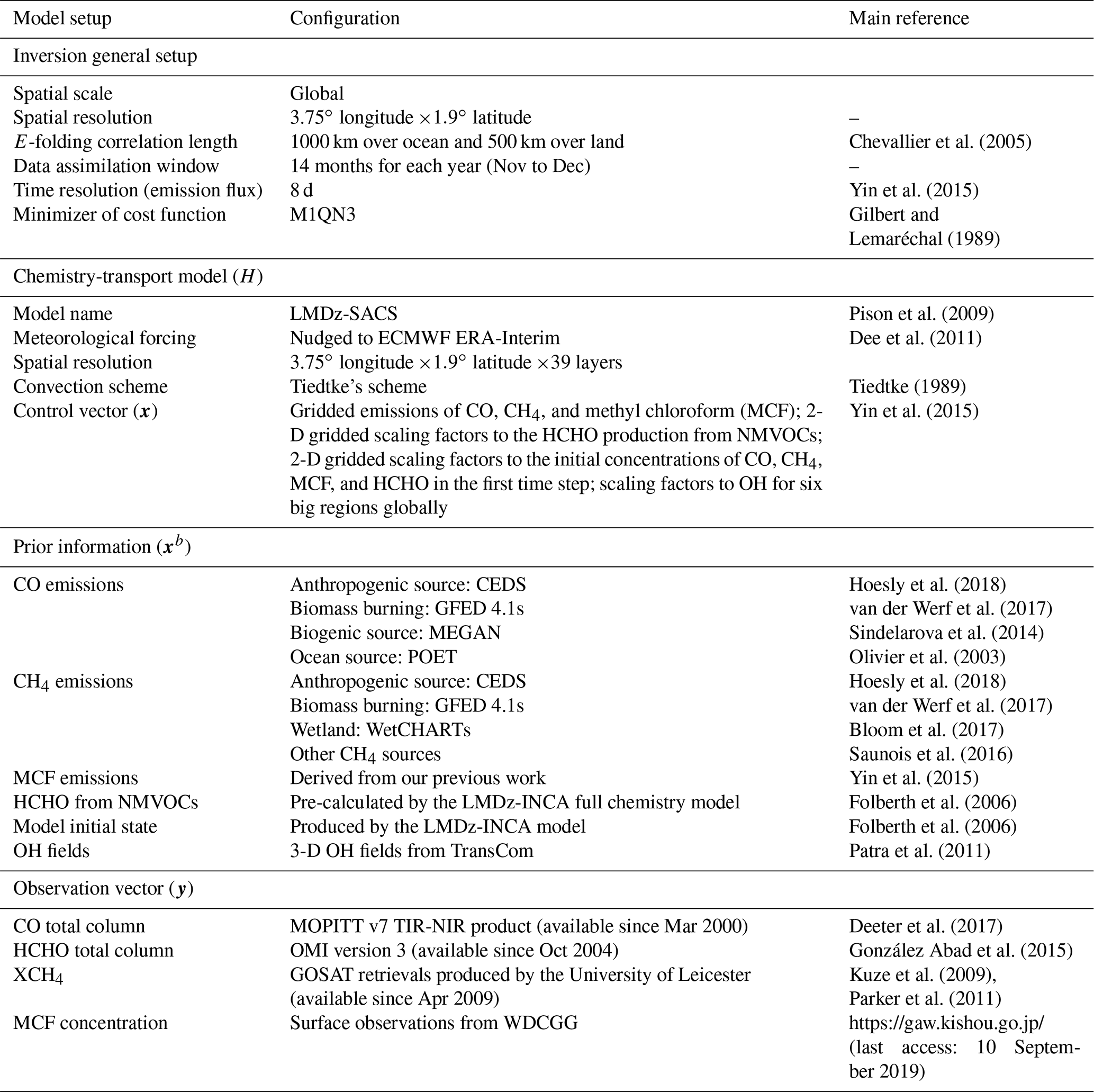
Atmospheric carbon monoxide (CO) concentrations have been decreasing since 2000, as observed by both satellite- and ground-based instruments, but global bottom-up emission inventories estimate increasing anthropogenic CO emissions concurrently. In this study, we use a multi-species atmospheric Bayesian inversion approach to attribute satellite-observed atmospheric CO variations to its sources and sinks in order to achieve a full closure of the global CO budget during 2000–2017. Our observation constraints include satellite retrievals of the total column mole fraction of CO, formaldehyde (HCHO), and methane (CH4) that are all major components of the atmospheric CO cycle. Three inversions (i.e., 2000–2017, 2005–2017, and 2010–2017) are performed to use the observation data to the maximum extent possible as they become available and assess the consistency of inversion results to the assimilation of more trace gas species. We identify a declining trend in the global CO budget since 2000 (three inversions are broadly consistent during overlapping periods), driven by reduced anthropogenic emissions in the US and Europe (both likely from the transport sector), and in China (likely from industry and residential sectors), as well as by reduced biomass burning emissions globally, especially in equatorial Africa (associated with reduced burned areas). We show that the trends and drivers of the inversion-based CO budget are not affected by the inter-annual variation assumed for prior CO fluxes. All three inversions contradict the global bottom-up inventories in the world's top two emitters: for the sign of anthropogenic emission trends in China (e.g., here % yr−1 since 2000, while the prior gives 1.3±0.4 % yr−1) and for the rate of anthropogenic emission increase in South Asia (e.g., here 1.0±0.6 % yr−1 since 2000, smaller than 3.5±0.4 % yr−1 in the prior inventory). The posterior model CO concentrations and trends agree well with independent ground-based observations and correct the prior model bias. The comparison of the three inversions with different observation constraints further suggests that the most complete constrained inversion that assimilates CO, HCHO, and CH4 has a good representation of the global CO budget, and therefore matches best with independent observations, while the inversion only assimilating CO tends to underestimate both the decrease in anthropogenic CO emissions and the increase in the CO chemical production. The global CO budget data from all three inversions in this study can be accessed from https://doi.org/10.6084/m9.figshare.c.4454453.v1 (Zheng et al., 2019).
- Article
(7578 KB) -
Supplement
(2260 KB) - BibTeX
- EndNote


Carbon monoxide (CO) is present in trace quantities in the atmosphere, but plays a vital role in atmospheric chemistry. CO is part of a photochemical reaction sequence driven by hydroxyl radical (OH) that links methane (CH4), formaldehyde (HCHO), ozone (O3), and carbon dioxide (CO2). The reaction of CO with OH accounts for 40 % of the removal of OH in the troposphere (Lelieveld et al., 2016) and governs the oxidizing capacity of the Earth's atmosphere. This reaction also makes CO an important precursor of O3 and affects the CH4 lifetime and abundance, which leads to an indirect positive radiative forcing of 0.2 W m−2 (Myhre et al., 2013). Since CO is heavily involved in the relationship between atmospheric chemistry and climate forcing, it is crucial to investigate its atmospheric burden, trends, and the underlying drivers.
Atmospheric CO concentrations following industrialization increased until around the late 1970s and have been decreasing since the 1990s, as shown by Greenland firn air records (Wang et al., 2012; Petrenko et al., 2013) and surface flask samples collected at few sites (Khalil and Rasmussen, 1994; Novelli et al., 2003; Gratz et al., 2015; Schultz et al., 2015). These few measurement points may not capture the global trend, given the short lifetime of CO being only several weeks. Since 2000, the atmospheric CO burden has been monitored globally and continuously by the CO vertical profiles and tropospheric total columns retrieved from the space-borne Measurements Of Pollution In The Troposphere instrument (MOPITT, Deeter et al., 2017). A declining trend is apparent in the MOPITT data, more pronounced in the Northern Hemisphere (Worden et al., 2013), where most of the global economic activity occurs, associated with a large amount of fossil fuel use and CO emissions from combustion processes. An intuitive explanation of the declining CO is that the improvement of combustion technologies (e.g., high-efficiency engines) has reduced CO emissions over time, but global bottom-up inventories oppositely estimate increasing anthropogenic CO emissions after 2000 because of the increasing fossil fuel consumption (Granier et al., 2011; Crippa et al., 2018; Hoesly et al., 2018). When prescribed with these inventories, atmospheric chemistry models fail to capture the observed rapid decline in atmospheric CO burdens globally (Petrenko et al., 2013; Strode et al., 2016).
Interpreting atmospheric CO trends requires accurate quantification of the global CO budget (Duncan et al., 2007), including surface sources, atmospheric sources (oxidation of hydrocarbons, known as CO chemical production), and atmospheric sinks. The surface sources include anthropogenic incomplete combustion of fossil fuels and biofuels (Hoesly et al., 2018), biomass burning (van der Werf et al., 2017), plant leaves (Tarr et al., 1995; Bruhn et al., 2013), and the ocean (Conte et al., 2019). Anthropogenic emissions depend on fuel type, fuel amount, combustion technology, and emission control devices (e.g., a catalytic converter for an automobile). Biomass burning emissions are caused by human-igniting or lightning fires on fire-prone landscapes such as savannas and forests. Fire intensities and CO emissions are sensitive to climatic conditions such as drought and heat waves (Chen et al., 2017), and are enhanced (e.g., deforestation) or suppressed (e.g., cultivation or forest fire suppression) by human activities. Peat fires produce larger CO emissions from incomplete combustion than open fires, especially in Indonesia (Yin et al., 2016). A small amount of CO is directly generated from plant leaves and marine biogeochemical cycling, which vary less from year to year than anthropogenic and biomass burning sources. However, large amounts of CO are produced from the oxidation of hydrocarbons from biogenic emissions that can vary due to climate and human land use changes. The oxidation by OH is the dominant sink of CO and gives CO a global average chemical lifetime of 1–3 months (Seinfeld and Pandis, 2006).
The contradiction between growing anthropogenic CO emissions in global bottom-up inventories (Granier et al., 2011; Crippa et al., 2018; Hoesly et al., 2018) and the MOPITT-observed declining CO since 2000 suggests three scenarios: (1) the CO sink has been increasing faster than the CO source, (2) the bottom-up inventories underestimate the improvement in combustion technology and the actual decrease in anthropogenic CO emissions, and (3) biomass burning emissions or CO chemical production have been decreasing rapidly. The first scenario is unlikely to be the main reason, because OH is considered well buffered in the atmosphere with a small inter-annual variation (Montzka et al., 2011; Naik et al., 2013; Voulgarakis et al., 2013), or slightly decreasing in the last decade, a process that may partly explain the renewed growth of atmospheric CH4 since 2007 (Rigby et al., 2017; Turner et al., 2017; McNorton et al., 2018). It is difficult to simply determine whether scenarios (2) and (3) play a big or small role because the estimates of anthropogenic and biomass burning CO emissions and trends are typically subject to large uncertainties. Although at first sight, growing anthropogenic emissions seemingly disagree with the observed declining CO, trends in biomass burning emissions, CO chemical production, and atmospheric transport all play a confounding role. This calls for a full closure of the atmospheric CO budget using the best available data and knowledge, which can be framed as an inverse problem that matches all available information within their uncertainties.
The main purpose of this study is to reconcile the observed and bottom-up estimated atmospheric CO budget since 2000, and to provide a self-consistent and accurate inversion-based data product of the global CO budget during 2000–2017. We use an atmospheric Bayesian inversion approach to infer the global CO budget, where surface CO emissions, CO chemical production, and CO sinks are optimized at a spatial resolution of 3.75∘ longitude ×1.9∘ latitude every 8 d. Three inversions (2000–2017, 2005–2017, and 2010–2017; see details in Sect. 2.2) are performed by assimilating multiple satellite observations of CO, HCHO, and CH4 in the inversion system as they become available in order to constrain the CO reaction sequence. One additional sensitivity inversion is conducted to use flat prior CO fluxes without inter-annual variations in order to assess the influence of prior variations on the CO budget estimates. Based on these inversion results, we investigate the magnitudes, trends, and drivers of the global CO budget from 2000 to 2017, helping to understand the observed remarkable decline in the atmospheric CO since 2000.
2.1 General methodology
The evolution of atmospheric CO concentrations with time in a 3-D atmospheric model grid box is expressed as the sum of multiple CO emission sources (SourceCO) minus the CO sink (SinkCO), which can be represented by the following Eq. (1).
The flux divergence term (υ⋅∇[CO]) represents the transport of CO into and out of each atmospheric model grid box, whose sum is equal to zero at the whole globe. ECO is the surface CO emission flux from different source sectors (i.e., anthropogenic, biomass burning, biogenic, and oceanic). and PNMVOCs→CO represent the CO chemical production from CH4 and non-methane volatile organic compounds (NMVOCs), respectively, oxidized by OH in the atmosphere. The CO chemical sink (kCO+OH(T)[CO][OH]) is calculated on the basis of CO ([CO]), OH ([OH]), and a temperature (T)-dependent rate (kCO+OH), and DepCO is the dry deposition of CO that contributes about 7 % of the CO total sink (Stein et al., 2014).
We use the global 3-D transport model of the Laboratoire de Météorologie Dynamique (LMDz) coupled with a simplified chemistry module, Simplified Atmospheric Chemistry assimilation System (SACS) (Pison et al., 2009), to simulate the atmospheric physical and chemical processes described in Eq. (1) except the dry deposition not represented by this model. An atmospheric Bayesian inversion framework is built upon the LMDz-SACS model (Chevallier et al., 2005, 2009), and satellite observations of the relevant trace gas species (CO, HCHO, and CH4) are assimilated to constrain the inversion system (Zheng et al., 2018a, b) given some prior information on the initial model state, surface emissions, CO chemical production, and OH field. Section 2.2 provides details of the atmospheric inversion approach and the model evaluation protocol, and Sect. 2.3 describes how we analyze the global CO budget using inversion results.
2.2 Atmospheric Bayesian inversion
The core of atmospheric Bayesian inversion is the minimization of the following cost function:
x is the control vector that gathers the target variables we seek to optimize, and xb is a prior guess of these variables assuming unbiased Gaussian error statistics represented by a covariance matrix B. y is the observation vector containing all the observation data assimilated to constrain the inverse problem; their error statistics are assumed to be unbiased and Gaussian with a covariance matrix R. H is the forward model (the combination of the LMDz-SACS model, a sampling operator, and an averaging kernel operator) that calculates the equivalent of the observation data in y based on the control vector x. The forward model error and the representation error caused by the mismatch between model and observation resolutions are also included in R, making R represent a combination of measurement, forward model, and representation errors. Configurations of the variables and vectors in Eq. (2) are summarized in Table 1 and Table S1 in the Supplement, most of which have already been described in our previous papers (Zheng et al., 2018a, b). To solve the inverse problem, forward and adjoint codes are iteratively run until sufficient convergence of the cost function (Eq. 2), and the last iteration with optimized model states gives us the best estimate that matches all available information within their uncertainties.
The inversion system has several updates compared to the version developed by the same research team a few years ago to study atmospheric CO trends (Yin et al., 2015). First, we use a higher-resolution transport model with finer horizontal grid cells ( compared to ) and more vertical layers (39 layers compared to 19 layers) than Yin et al. (2015) used. Second, we assimilate the MOPITT version 7 data as an observation constraint, which is improved with respect to retrieval biases and bias drift compared to the previously used version 6 data (Deeter et al., 2017). Third, we use the latest global bottom-up emission inventories as prior, including the Community Emissions Data System (CEDS, Hoesly et al., 2018) for the anthropogenic source and the Global Fire Emissions Database (GFED) 4.1s for the biomass burning source. The regional studies of Zheng et al. (2018a, b) used the same configuration than here, except that they assimilated in situ measurement for CH4 rather than satellite retrievals.
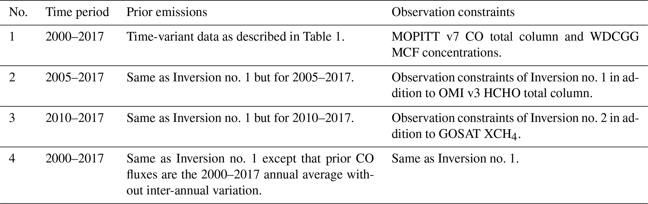
We perform four inversion simulations with our inversion system (Table 2). Inversion no. 1 (2000–2017) is constrained by CO total columns derived from the MOPITT version 7 TIR-NIR retrievals; Inversion no. 2 (2005–2017) is constrained by both the MOPITT CO column and the Ozone Monitoring Instrument (OMI) version 3 HCHO column; and Inversion no. 3 (2010–2017) is additionally constrained by Greenhouse gases Observing SATellite (GOSAT) column-averaged dry air mole fractions of CH4 (XCH4). All three inversions also assimilate in situ measurement of methyl chloroform (MCF) to help constrain OH (Yin et al., 2015), but the rapidly declining levels of MCF in the atmosphere make this constraint progressively ineffective (e.g., Liang et al., 2017). Factorial simulations constrained by MOPITT CO, OMI HCHO, and GOSAT XCH4 allow us not only to better constrain the photochemical reaction sequence of CO, but also to facilitate a quantitative assessment of potential uncertainties in the inversion CO budget relating to the use of different observation constraints. We also do a sensitivity Inversion no. 4 (2000–2017) with the same observation constraints as Inversion no. 1 but flat prior surface CO emissions without any inter-annual variability to check whether the derived CO budget is robust to the inter-annual variation of the prior CO fluxes.
Inversion results of the optimized CO concentration in the atmosphere are evaluated against independent ground-based observations from the World Data Centre for Greenhouse Gases (WDCGG, https://gaw.kishou.go.jp/, last access: 10 September 2019) and the Total Carbon Column Observing Network (TCCON, Wunch et al., 2011). The WDCGG provides measurements of surface CO concentrations through in situ and flask sample measurements, and the TCCON provides retrievals of the column-averaged dry air mole fraction of CO (XCO). We collect observation data from 110 sites in WDCGG (Table S2) and from 32 sites in TCCON (Table S3; station names and references are shown in Appendix Fig. A1), which cover the whole globe (Fig. A1). To do the evaluation, we first sample the model at the location and time of the observation data and then calculate the average values and annual trends for both model and observation. The annual trends are estimated on the basis of monthly time series using a curve fitting method (https://www.esrl.noaa.gov/gmd/ccgg/mbl/crvfit/crvfit.html, last access: 10 September 2019), which is also used in Zheng et al. (2018a). p values and 95 % confidence intervals are given to assess the robustness of the estimated trends. The metrics used for evaluation include normalized mean bias (NMB), root mean square error (RMSE), Pearson's correlation (R), and the regression slope between model and observation among all surface sites.
2.3 Atmospheric CO budget
The picture of the atmospheric CO budget derived from our inversions includes surface fluxes (the sum of direct emissions from different source sectors and of dry deposition), CO chemical production, and CO chemical sink. Given the marginal role played by dry deposition (about 20 % of the direct emissions, Stein et al., 2014), the inferred surface fluxes will be assumed to be made of direct emissions only in the following. The CO chemical production and chemical sink are direct outputs from the inverse system, which calculates the CO yield from the oxidation of CH4 and of NMVOCs and the CO oxidation sink with the linearized chemistry scheme in each model grid box at each time step of the model simulation.
To obtain sectoral surface emission fluxes, we multiply the optimized 8-daily surface total fluxes by the proportion of each sector in each model grid cell as given by the prior (Jiang et al., 2017; Yin et al., 2016; Zheng et al., 2018b). We distinguish between four source sectors, anthropogenic, biomass burning, biogenic, and oceanic, which have rather distinct spatial–seasonal patterns in CO emission distributions. Without considering the oceanic emission, 96 % of the CO emissions on land are distributed on grid cells with a dominant emission source (i.e., a sector that contributes more than 50 % of CO flux in that grid). Further, 85 % of CO emissions on land are distributed in grid cells where such a dominant source accounts for more than 65 % of the CO total flux. The distinct seasonal evolutions of different sectors also help attribute emissions to one specific source sector. For example, the biomass burning in Africa typically accounts for 80 %–90 % of surface CO emissions in the dry season (Zheng et al., 2018b). This local source homogeneity reduces the attribution bias of sectoral CO fluxes, although it cannot eliminate all biases. To minimize remaining biases, we focus on annual emission anomalies by removing the multiannual average or calculating linear trends to reduce the systematic errors. This makes it possible to directly compare the inversion-based emissions with bottom-up inventories to analyze the underlying emission drivers (Sect. 4.2).
We also collect previous top-down inversion estimates of the global CO budget from the scientific literature (Table S4). These studies used older versions of MOPITT retrievals (or other satellite data) and coarser-resolution transport models, and they did not have the capability of multi-species constraints. Despite a different observation data quality and inversion model setup, it is still meaningful to do such a review to visualize the evolution of the inversion-based global atmospheric CO budget.
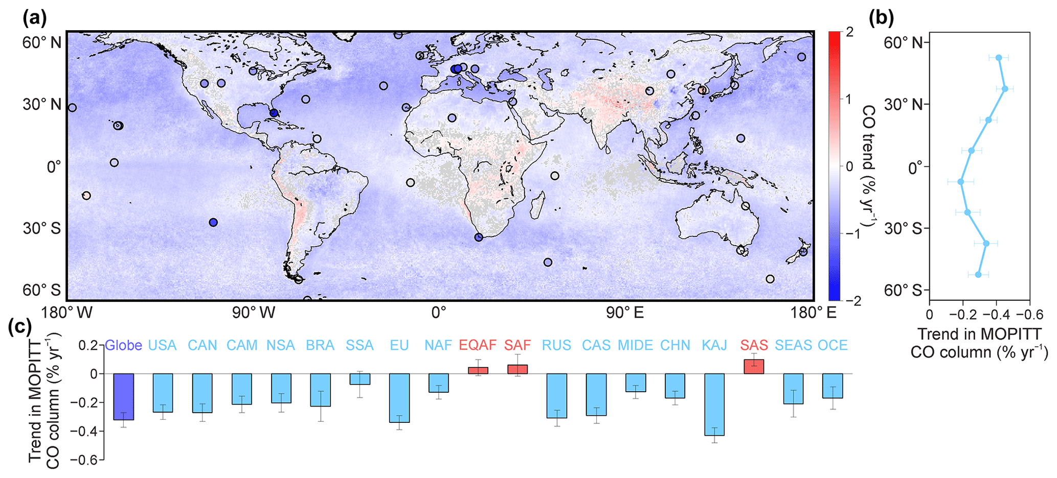
Figure 1Trends in the abundance of atmospheric CO from 2000 to 2017. The map (a) shows the 2000–2017 trends in MOPITT CO total columns at the spatial resolution of ∘ with the WDCGG sites (dots) that have a continuous measurement during 2000–2017. The color of the WDCGG dots represent the trends in surface CO concentrations. The curve in (b) shows the trends in MOPITT CO columns by latitude band. The bars in (c) show regional CO column trends (region split refers to Fig. A1). The trends in (a), (b), and (c) are all estimated on the basis of monthly time series using a curve fitting method as described in Zheng et al. (2018a). The grey color in the map (a) indicates the areas or dots without statistically significant trends (p≥0.05), and the error bars in (b) and (c) represent the 95 % confidence intervals. Fig. S1 in the Supplement presents the trends of MOPITT CO columns from 2005 to 2017 (Fig. S1a) and from 2010 to 2017 (Fig. S1b), respectively.
3.1 Observed declining CO since 2000
Tropospheric CO columns observed by MOPITT v7 declined at an average rate of % yr−1 (p < 0.01; numbers with ± signs are 95 % confidence limits from a linear fit) from 2000 to 2017 over the whole globe (Figs. 1a, S1). This trend, equivalent to molec. cm−2 yr−1, is much larger than the retrieval bias drift of molec. cm−2 yr−1 in the MOPITT v7 TIR-NIR product (Deeter et al., 2017), indicating that the observed downward trend is robust to satellite retrieval errors (Worden et al., 2013). The distributed ground-based sites of the WDCGG network (dots in Fig. 1a) also measure rapidly decreasing surface CO concentrations during 2000–2017, broadly consistent with the negative trends of the MOPITT CO columns. The sites located on or near continents, more affected by land sources upwind, generally show faster CO concentration declines than the MOPITT CO columns, while the background sites, especially those over islands, agree better with MOPITT observations. The TCCON-observed XCO also presents consistent declining trends with MOPITT (Fig. S2).
The trends in MOPITT CO columns reveal heterogeneous spatial patterns (Fig. 1b and c). The largest decrease is seen in the northern mid-latitudes (30–60∘ N), where Canada (CAN), the USA, Europe (EU), Russia (RUS), and China (CHN) all present statistically significant declining trends (Fig. 1c). The tropical region (30∘ S–30∘ N) has a smaller decrease in CO columns due to some increasing trends existing over South Asia (SAS) and over a large part of Africa. South Asia is the only region that has a statistically significant trend of rising CO columns since 2000 according to our region splitting (Fig. A1). The African continent presents both increasing and decreasing CO columns that compensate each other and therefore lead to no statistically significant trends over equatorial Africa (EQAF) and southern Africa (SAF) (Fig. 1c). This is consistent with ground-based observations at Ascension Island, UK (ASC, Table S2), located downwind of the West African coast that sees CO plumes from Africa. The southern mid-latitudes (30–60∘ S) primarily consist of the ocean with very few lands, where the MOPITT and WDCGG observations both show consistently moderately decreased CO abundance.
3.2 Global atmospheric CO budget
3.2.1 MOPITT-constrained inversion
Inversion no. 1, constrained by MOPITT v7 CO columns, estimates that the global annual CO source was 2.6×10³ Tg CO yr−1 on average and decreased at a rate of Tg CO yr−2 (p < 0.01) during 2000–2017 (Table 3). The chemical sink of CO by reaction with OH is estimated as 2.6×10³ Tg CO yr−1 with a declining trend of Tg CO yr−2 (p < 0.01). The steady declining CO source breaks the source–sink balance of CO in the atmosphere, makes the CO source slightly smaller than its sink, and therefore drives the atmospheric CO burden down from 2000 to 2017. The reduced CO source further leads to a comparable decline in the CO sink due to a relatively stable OH burden in the troposphere.
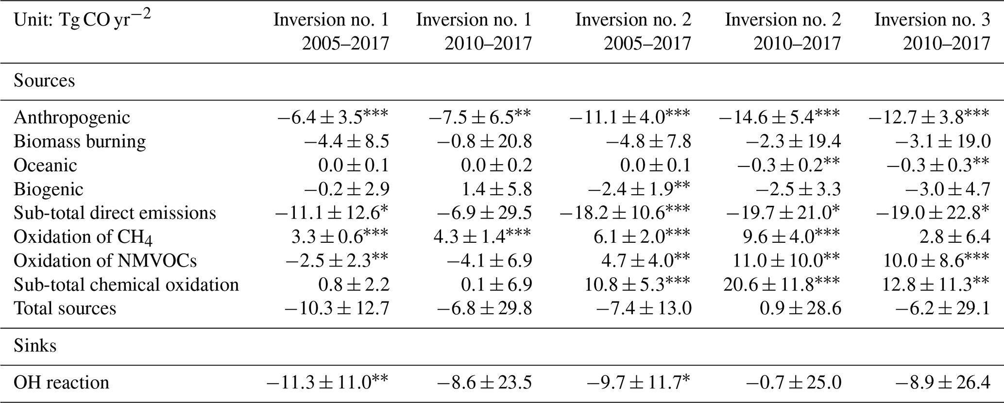
Table 3Global atmospheric carbon monoxide budget during 2000–2017. Average CO budget (103 Tg CO yr−1), coefficient of variation (CV, %), and absolute trends from 2000 to 2017 (Tg CO yr−2) are derived from Inversion no. 1 (see Table 2). Relative trends (% yr−1) with 95 % confidence limits are shown for both Inversion nos. 1 and 4 (no inter-annual variation in the prior CO flux). Significant trends are marked by asterisks (*p < 0.1, , and ).
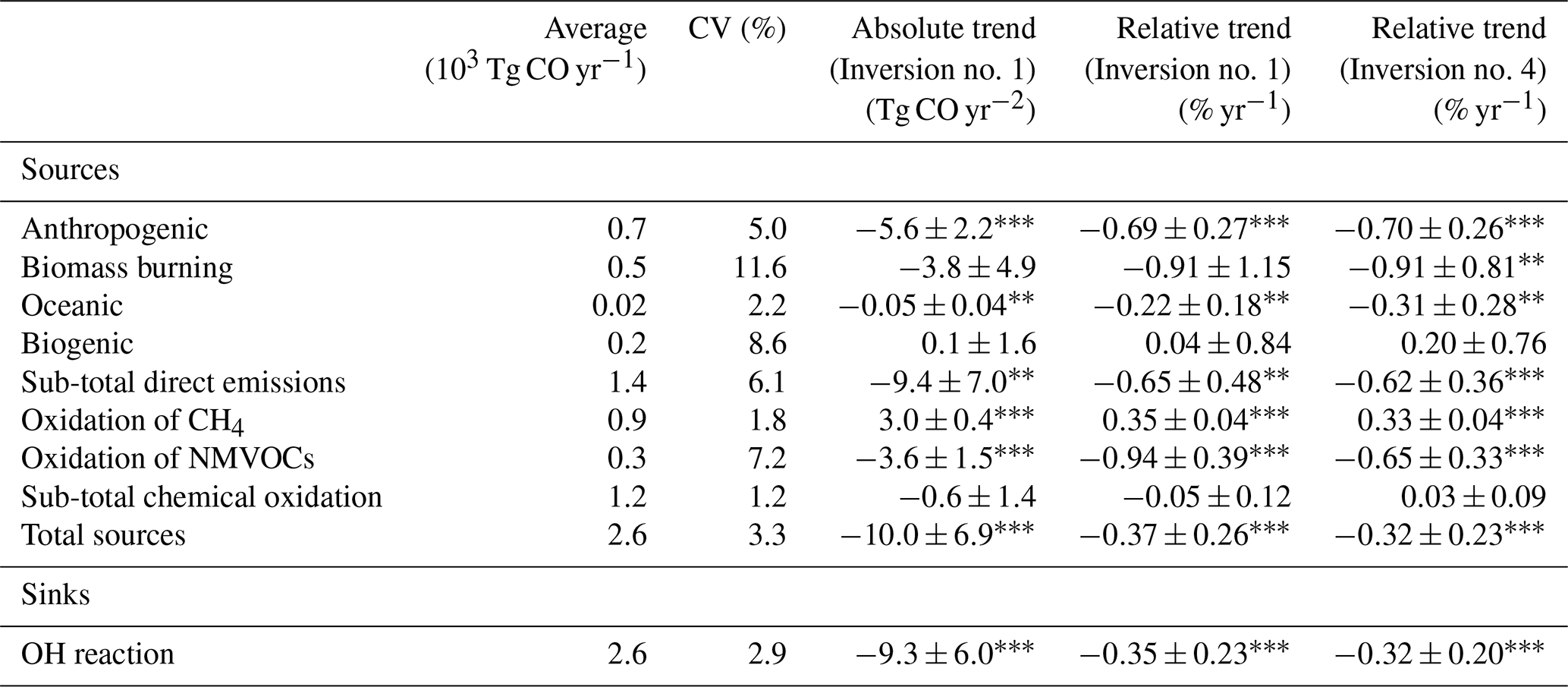
The global CO source is spread roughly equally between direct emissions from the Earth's surface (1.4×10³ Tg CO yr−1) and the chemical production in the atmosphere (1.2×10³ Tg CO yr−1). The direct emissions are estimated to have decreased by 9.4±7.0 Tg CO yr−2 (p=0.01), driven by decreasing anthropogenic ( Tg CO yr−2, p < 0.01) and biomass burning ( Tg CO yr−2, p=0.11) sources. The trend in biomass burning emissions has a large p value, which means statistical non-significance due to a large year-to-year variation (coefficient of variation, CV =11.6 %), especially the peak emissions from Southeast Asia (SEAS) at the end of 2015 caused by the 2015–2016 El Niño event (Yin et al., 2016; Liu et al., 2017). The oceanic and biogenic sources account for only 15 % of surface CO emissions with a small inter-annual variability (CV =2.2 % and 8.6 %, respectively), and therefore they have little effect on the trend of the CO total source. In contrast to declining direct emissions, the CO chemical production is estimated to have remained flat (CV =1.2 %), resulting from the compensation between increasing yields from CH4 oxidation (3.0±0.4 Tg CO yr−2, p < 0.01) and decreasing yields from NMVOC oxidation ( Tg CO yr−2, p < 0.01).
Three variables determine the global CO sink as discussed in Eq. (1): kCO+OH(T), [CO], and [OH]. Tropospheric CO columns measured by MOPITT declined at a relative rate of % yr−1 (p < 0.01) during 2000–2017, highly consistent with the relative trend in the estimated CO sink ( % yr−1, p < 0.01). This suggests that decreasing CO concentrations are the primary driver of the declining CO sink and dominate over the influence from the possible changes in OH and reaction rate.
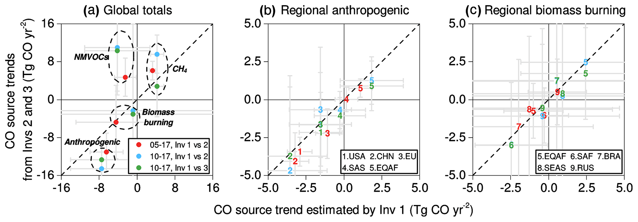
Figure 2Comparison of inversion-based CO source trends between Inversion nos. 1, 2, and 3. The comparison is conducted between Inversion nos. 1 and 2 for 2005–2017 (red dot), between Inversion nos. 1 and 2 for 2010–2017 (blue dot), and between Inversion nos. 1 and 3 for 2010–2017 (green dot). The global totals are presented in (a), and the top five emitters (region definition refers to Fig. A1) of regional anthropogenic and biomass burning emissions are presented in (b) and (c), respectively. In all these figures, the CO source trends derived from Inversion no. 1 are presented along with the x axis, and the CO source trends from Inversion nos. 2 and 3 are presented along with the y axis. The error bars for x and y (grey lines) are 95 % confidence intervals of the estimated linear trends.
3.2.2 Influence of OMI HCHO and GOSAT XCH4 constraints
Inversion nos. 2 and 3 assimilated OMI HCHO and GOSAT XCH4 in the inverse system to directly constrain the reactants of CO chemical production. These two inversions make a small difference (< 10 % for a single year and < 2 % for the multiannual mean) in the global CO budget estimates compared to Inversion no. 1 (Table S5), and all three inversions estimate a slightly smaller CO source than the CO sink in most of the years between 2000 and 2017. However, the three inversions reveal different declining trends (Table 4; Fig. 2). Inversion no. 2 estimates that the global CO source and sink decreased at the rates of Tg CO yr−2 (p=0.24) and Tg CO yr−2 (p=0.09), respectively, from 2005 to 2017, slightly slower than Inversion no. 1-estimated trends of Tg CO yr−2 (p=0.10) and Tg CO yr−2 (p=0.05) in the same period. The large p values for trends during 2005–2017 indicate a large inter-annual variability, mainly caused by the significant biomass burning emissions from peat fires in Indonesia during the 2015–2016 El Niño event (Sect. 3.3). The slower decline in the CO total source estimated by Inversion nos. 2 and 3 is primarily due to the growing CO production (Fig. 2a), in contrast to the flat CO chemical production estimated by Inversion no. 1. For example, Inversion no. 2 estimates that the CO production increased by 10.8±5.3 Tg CO yr−2 (p < 0.01) during 2005–2017, and Inversion no. 3 estimates a growing CO production by 12.8±11.3 Tg CO yr−2 (p=0.03) during 2010–2017.
Table 4Absolute trends in the global atmospheric carbon monoxide budget. Absolute trends (Tg CO yr−2) with 95 % confidence limits are estimated for the time period of 2005–2017 and 2010–2017 using Inversion nos. 1, 2, and 3 (see Table 2). Significant trends are marked by asterisks (* p < 0.1, p < 0.05, and p < 0.01).
Direct anthropogenic CO emissions are estimated to decline faster in Inversion nos. 2 and 3 (Table 4 – those trends being compared during the same overlapping periods for inversions in this table). Inversion no. 1 estimates that anthropogenic CO emissions declined by Tg CO yr−2 (p < 0.01) during 2005–2017, while Inversion no. 2 shows a steeper decline of Tg CO yr−2 (p < 0.01). During 2010–2017, Inversion nos. 2 and 3 estimate declining rates of Tg CO yr−2 (p < 0.01) and Tg CO yr−2 (p < 0.01), respectively, both faster than the Inversion no. 1-estimated trend of Tg CO yr−2 (p=0.03). For the top five emitters of anthropogenic CO (Fig. 2b), we see faster declines in the USA, CHN, and EU and slower growth over SAS and EQAF than those present in Inversion no. 1. However, biomass burning emissions and trends tend to remain almost unchanged in Inversion nos. 2 and 3 (Table 4; Fig. 2c).
3.2.3 Best estimate between different inversions
Inversion nos. 1, 2, and 3 all clearly suggest that decreased surface emissions from anthropogenic and biomass burning sources are major drivers of the declining global CO source during 2000–2017; however, they estimate different trends in anthropogenic CO emissions and CO chemical production. This suggests that the additional observation constraints related to the CO reaction sequence alter the inversion-estimated trends of the global CO budget.
Inversion no. 1 is capable of separating the trend of the CO total source from the trend of the CO total sink, broadly consistent with the results derived from Inversion no. 2 and Inversion no. 3, but the contribution of reduced anthropogenic sources to the declining CO emissions seems to be underestimated in Inversion no. 1 because the increasing CO chemical production is not directly constrained in that inverse configuration. The increased CO chemical production is reflected by the growing HCHO in the atmosphere, which is an intermediate reaction product in the oxidation of hydrocarbons. Tropospheric HCHO columns as observed by OMI have been reported to keep growing over China, India, and part of the USA over the last decade (De Smedt et al., 2010; Zhu et al., 2017; Shen et al., 2019), probably related to strong increases in anthropogenic NMVOC emissions. The bias of Inversion no. 1 that does not constrain the HCHO and CO production is region-dependent, but is most evident in anthropogenic source regions (e.g., China and the US) where rapidly increasing man-made NMVOC emissions dominate over relatively stable biogenic NMVOCs. With additional OMI HCHO and GOSAT XCH4 constraints, the CO chemical production in these regions is estimated to increase instead of being flat, which further leads to a faster decrease in the estimated anthropogenic CO emissions to maintain the overall declining CO burden in the atmosphere. In biomass burning regions where biogenic NMVOC emissions are relatively stable, the estimates of biomass burning CO emissions are quite consistent across the three different inversions.
The most realistic inversion estimate of the global CO budget should be the one with sufficient constraints not only on the atmospheric CO abundance, but also on the CO chemical production. The CO chemical production is an important term of the CO budget trends, as it experienced a steady increase due to growing HCHO and CH4 concentrations in the atmosphere. Constraining the CO chemical production can correct the inversion system that may inaccurately attribute some of the decreases in the CO source to the CO chemical production. Therefore, it is reasonable to think that Inversion no. 3 has a more realistic representation of the source splitting between anthropogenic emissions and chemical production in the global CO budget than Inversion no. 2 does, and Inversion no. 2 is better than Inversion no. 1. It is appropriate to use Inversion no. 3 and Inversion no. 2 for the trend analysis, but these inversions are limited to short periods. If Inversion no. 1 has to be used due to its long-term temporal coverage, caution needs to be taken that the decreasing trends of anthropogenic CO emissions are probably underestimated and the increasing trends of CO chemical production are not well separated over anthropogenic source regions. For the trend analysis in this paper, we present all the estimates from Inversion nos. 1, 2, and 3 for completeness. The global CO budget data derived from all three inversions can be found at the data repository of https://doi.org/10.6084/m9.figshare.c.4454453.v1 (Zheng et al., 2019).
3.2.4 Comparison with the prior CO budget
The comparison with the prior modeled CO budget (Table S6) shows that the inversion system adjusts both the magnitudes and trends of the CO source and CO sink. Inversion nos. 1, 2, and 3 exhibit similar estimates in the global CO source, which are 15 % ( Tg CO yr−1) larger than the prior CO flux on average, including 1.1×10² Tg CO yr−1 from anthropogenic sources, 1.1×10² Tg CO yr−1 from biomass burning sources, and 0.9×10² Tg CO yr−1 from biogenic sources. The increment of 15 % is within the uncertainty range of bottom-up CO inventories, which are typically subject to a 1-sigma uncertainty between 26 % and 123 % for top emitting anthropogenic regions and countries (Crippa et al., 2018). The inversion-based CO sink is 14 % higher than the prior estimates, equivalent to another 3.2×10² Tg CO yr−1 loss. For trends, the prior results exhibit an increasing CO source (3.6±3.8 Tg CO yr−2, p=0.07) that could result in a growing atmospheric CO burden from 2000 to 2017, disagreeing with the observed declining CO since 2000. The inversion results reverse the upward trend in prior anthropogenic emissions to a rapid downward trend and estimate larger decreases in biomass burning emissions.
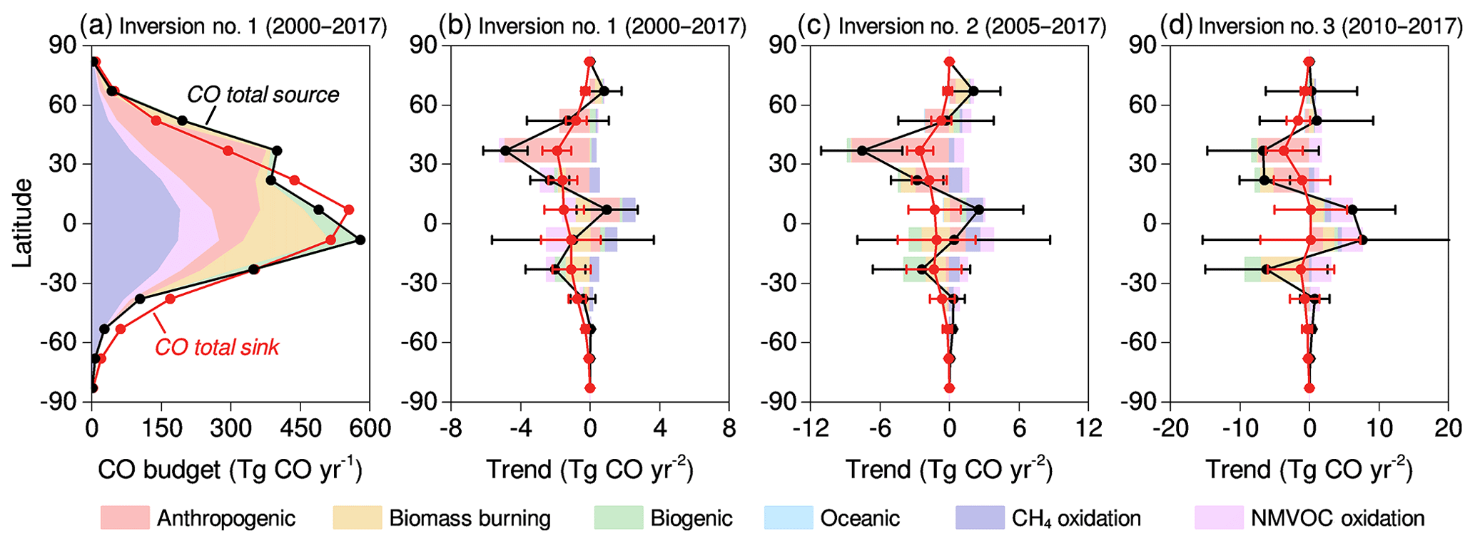
Figure 3Global CO budget and trends by latitude band. The global CO source (black curve and stacked chart) and sink (red curve) derived from Inversion no. 1 are presented in (a) for every 15∘ latitude band. The budget trends with 95 % confidence intervals are estimated for 2000–2017 using Inversion no. 1 (b), for 2005–2017 using Inversion no. 2 (c), and for 2010–2017 using Inversion no. 3 (d). The trends are estimated using the linear least squares fitting method based on annual time series for each 15∘ latitude band.
3.3 Regional atmospheric CO budget
3.3.1 Regional distribution
The global CO source, the sum of surface emissions and chemical production, follows a bimodal distribution by latitude (Figs. 3a, 4a, S3a, S4a). The highest peak is in tropical regions (30∘ S–30∘ N), where 70 % of the global CO source is located, including 83 % of biomass burning emissions, 75 % of CO chemical production, and 50 % of anthropogenic emissions. The regions closest to the Equator, such as South America, equatorial Africa, Southeast Asia, and northern Australia, are responsible for most of the biomass burning emissions (Fig. 5c) and of the CO chemical production. The anthropogenic emission hotspots are equatorial Africa, South Asia, and South China (Fig. 5a). The other peak latitude band of the CO source is the northern mid-latitudes (30–60∘ N), which account for 23 % of the global CO source, dominated by the anthropogenic emissions from the US, Europe, and China (Fig. 5a). On average, 47 % of the global anthropogenic CO emissions are distributed within 30–60∘ N.
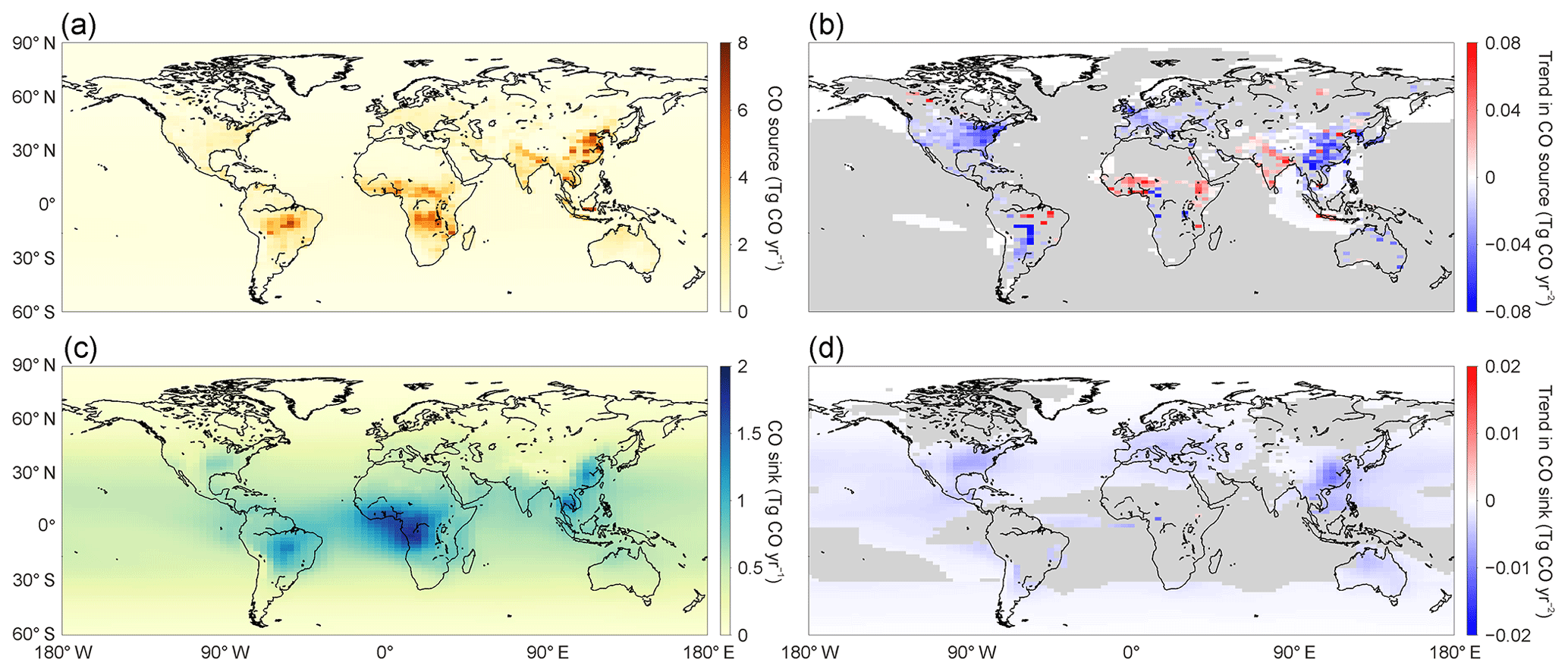
Figure 4Spatial distribution of the global CO budget and 2000–2017 trends. Annual average CO total source and sink during 2000–2017 are shown at the spatial resolution of 3.75∘ longitude ×1.9∘ latitude in (a) and (c), respectively, and linear trends of each grid cell are shown in (b) and (d), which are estimated using the linear least squares fitting method based on annual time series. Grey color in (b) and (d) indicates the areas without statistically significant trends (p≥0.05). All data shown in this figure are derived from Inversion no. 1 results. The spatial–temporal distributions derived from Inversion no. 2 and Inversion no. 3 are shown in Figs. S3 and S4, respectively.
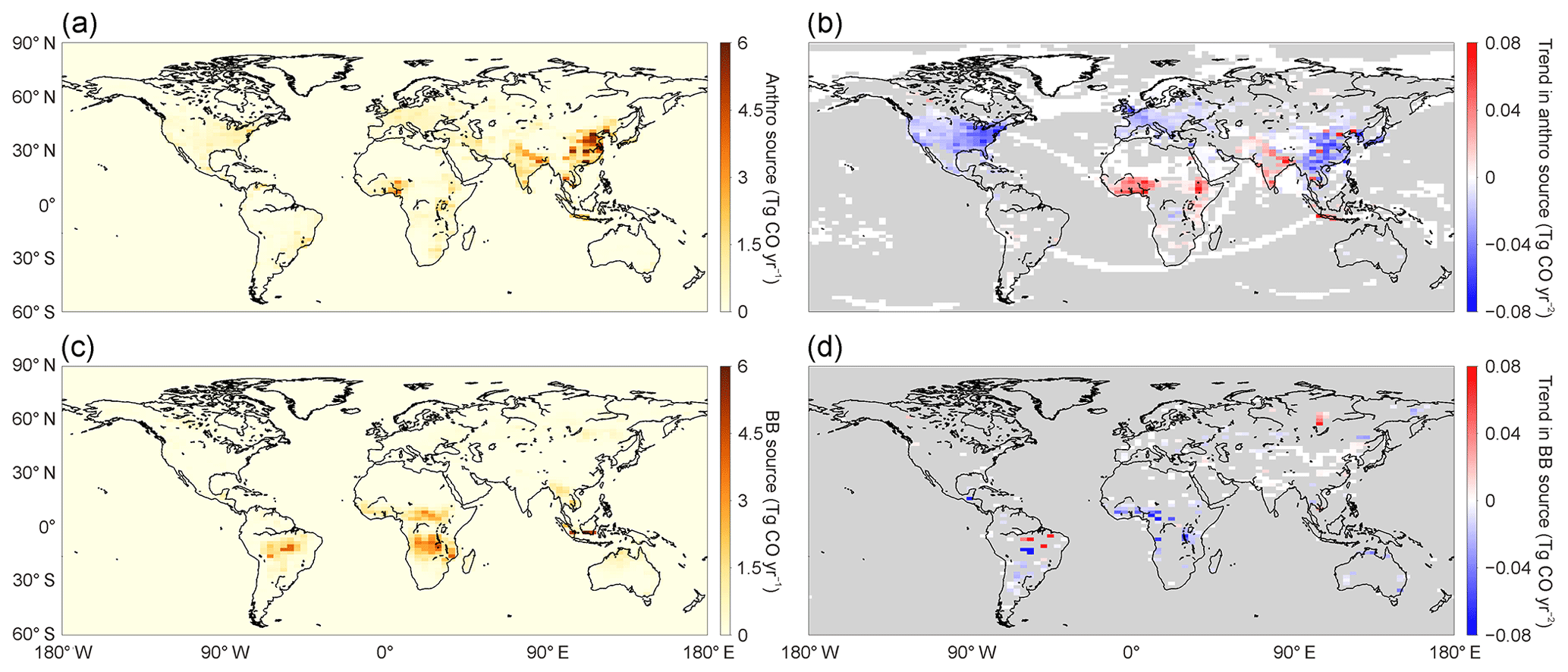
Figure 5Spatial distribution of anthropogenic and biomass burning CO emissions and the 2000–2017 trends. Annual average CO emissions from anthropogenic and biomass burning sources are shown at the spatial resolution of 3.75∘ longitude ×1.9∘ latitude in (a) and (c), respectively, and linear trends of each grid cell are shown in (b) and (d), which are estimated using the linear least squares fitting method based on annual time series. Grey color indicates the areas without anthropogenic and biomass burning emissions or without statistically significant trends (p≥0.05). All data shown in this figure are derived from Inversion no. 1 results.
The global CO sink presents an asymmetrical distribution around the Equator that is 30 % larger in the Northern Hemisphere than that in the Southern Hemisphere, due to the higher CO levels in the Northern Hemisphere (Figs. 3a, 4c, S3c, S4c). The tropical regions (30∘ S–30∘ N) that have both the largest CO source and OH concentration (Lelieveld et al., 2016) account for 71 % of the global CO sink, consistent with the proportion of CO source distributed over this region. The northern mid-latitudes (30–60∘ N) account for only 17 % of the global CO sink but 23 % of the CO source due to a much lower OH concentration than in the tropical troposphere. The southern mid-latitudes (30–60∘ S) account for 9 % of the global CO sink, corresponding to 5 % of the global CO source located in this region. A strong CO sink is also evident near coastlines over the ocean (e.g., west of the African continent), mainly due to the fact that the CO transported out of lands driven by prevailing winds further react with OH over the ocean.
For trends, the northern mid-latitudes (30–60∘ N) show the sharpest declines in both CO source and CO sink, consistently presented in Inversion nos. 1 (Fig. 3b), 2 (Fig. 3c), and 3 (Fig. 3d). The decline in the CO source is most evident in the US, Europe, and China (Figs. 4b, S3b, S4b), mainly caused by reduced anthropogenic sources (Fig. 5b). This drives the largest regional decrease in CO total columns between 30 and 60∘ N as seen by MOPITT (Fig. 1) and also leads to a significantly reduced CO sink. The tropical region (30∘ S–30∘ N) exhibits both increased and decreased CO sources over different continents. The increased sources over South Asia and equatorial Africa are both driven by the exponential growth in anthropogenic emissions (Fig. 5b), which partially offsets the decreasing biomass burning emissions in equatorial Africa and South America (Fig. 5d). The increase in the CO chemical production is seen over the whole tropical region, as shown in Fig. 3c and d. However, the estimated CO sink lacks statistically significant trends in the majority of the tropical region, and the continents with fast-growing CO sources (e.g., South Asia, equatorial Africa) lead to increased CO total columns (Fig. 1), although the global background concentrations are rapidly decreasing.
3.3.2 Anthropogenic emissions
The top five emitters of anthropogenic CO are CHN, SAS, USA, EQAF, and EU, where large amounts of fossil fuel and biofuel are burned in industrial, transportation, and residential facilities. These five regions are estimated to account for more than 60 % of the global anthropogenic CO emissions (Tables S7, S8, S9) and can explain more than 80 % of the global downward trend from 2000 to 2017 (Fig. 6a). CHN, USA, and EU are estimated to have reduced their emissions rapidly, which more than offsets the increasing emissions from SAS and EQAF. Emissions from all the other regions contribute much less to total anthropogenic emissions, and most of the emission changes are not statistically significant (p > 0.1) and therefore have little influence on the anthropogenic CO emissions trends.
A comparison with the bottom-up anthropogenic inventory CEDS that we use as prior shows that the Inversion no. 1 estimates stay close to CEDS over CHN, SAS, and the USA, but have larger values in regions with medium-sized emissions (20–50 Tg CO yr−1), such as in the EU and EQAF (Fig. 7a; Table S7). The inversion-based larger emissions in those regions help correct the biases of the prior modeled CO concentrations with respect to independent surface observations (Sect. 3.4). For the 2000–2017 trend (Fig. 7b), the discrepancy between Inversion no. 1 and CEDS mainly occurs for the top two emitters, CHN and SAS, although their long-term averages agree well. Inversion no. 1 shows that CHN emissions decreased and SAS emissions increased modestly, while both of these two regions are allocated a rapid growth in CEDS. As Inversion no. 1 tends to underestimate the decrease and to overestimate the increase in anthropogenic emissions (Sect. 3.2), the CEDS inventory probably has large biases in emission trend estimates over CHN and SAS, which is the main reason why it estimates growing anthropogenic emissions globally (Table S6) and cannot match the observed declining CO when used in the input of our LMDz-SACS model. This is consistent with the finding of Strode et al. (2016), who performed global CO modeling with a different model and inventory.
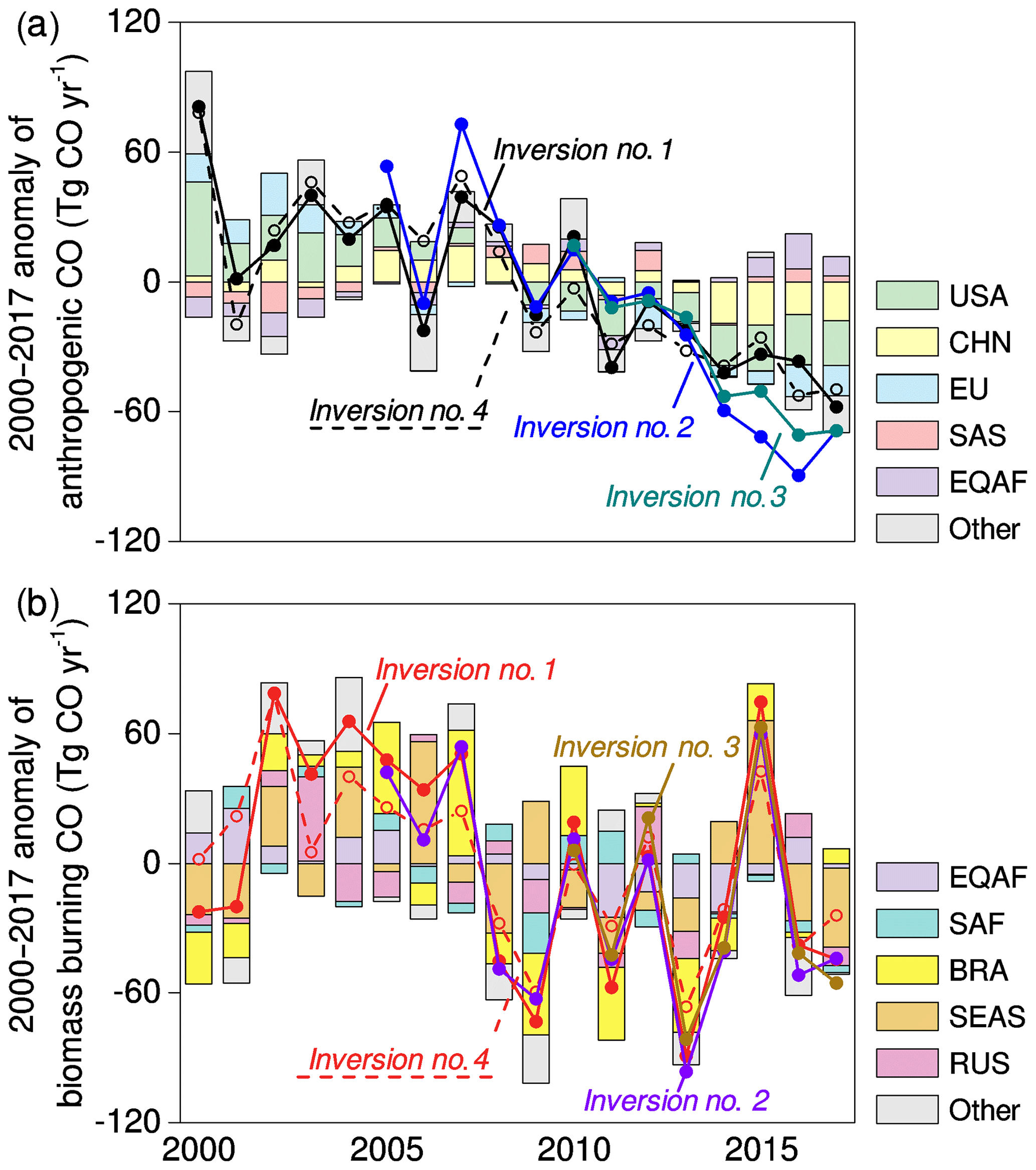
Figure 6Global CO emission anomalies from 2000 to 2017. Anthropogenic (a) and biomass burning (b) emission anomalies are presented with global totals derived from Inversion nos. 1 to 4 (curves) as well as regional emission anomalies (stacked bar) derived from Inversion no. 1, including the top five emitters and the sum of all the other regions. For Inversion no. 1 and Inversion no. 4, the emission anomalies are calculated by removing the 2000–2017 average calculated from their own time series data. For Inversion no. 2 and Inversion no. 3, the emission anomalies are calculated by removing the 2000–2017 average calculated from Inversion no. 1.
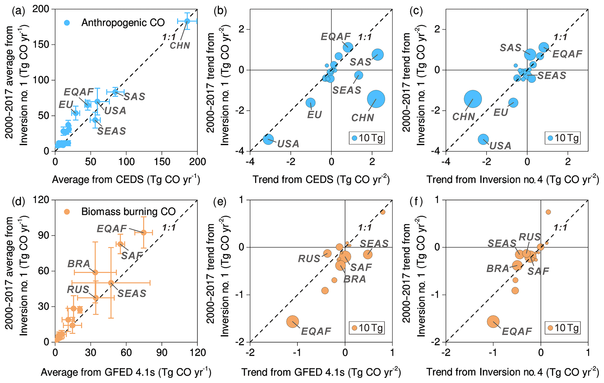
Figure 7Comparison between Inversion no. 1 emission estimates with the prior emissions and Inversion no. 4 estimates. Annual average regional anthropogenic emissions (Tg CO yr−1, blue dots in a) are compared between Inversion no. 1 (y axis) and the CEDS estimate (x axis) with coefficients of variation as error bars. The linear trends (Tg CO yr−2) in regional anthropogenic emissions (blue dots in b and c) are compared between Inversion no. 1 (y axis in b and c) and the CEDS inventory (x axis in b) and Inversion no. 4 estimate (x axis in c), respectively, with the area of each dot proportional to annual average emissions derived from Inversion no. 1. (d), (e), and (f) are similar to (a), (b), and (c), respectively, but for biomass burning CO emissions.
3.3.3 Biomass burning emissions
Inversion nos. 1, 2, and 3 consistently estimate declining biomass burning CO emissions (Fig. 6b), primarily driven by five regions (EQAF, SAF, Brazil – BRA, SEAS, and RUS) that account for more than 70 % of global biomass burning CO (Tables S10, S11, S12). Based on Inversion no. 1 results, EQAF presents a declining trend of Tg CO yr−2 (p < 0.01, Table S10) during 2000–2017, while emissions in the other four regions fluctuate. The large inter-annual variability makes the assessment of a trend more uncertain, especially given high emissions during extreme drought years. For example, the 2010 emissions are estimated significantly higher than the 2009 emissions due to the suddenly rising emissions in BRA caused by drought in the Amazon forest (Lewis et al., 2011; Xu et al., 2011). The 2015 emissions are estimated close to the maximum since 2000 due to fire anomalies in SEAS and BRA as a consequence of record-breaking drought during the 2015–2016 El Niño event (Jiménez-Muñoz et al., 2016; Yin et al., 2016; Liu et al., 2017). Besides, the EU and Korea and Japan (KAJ) both present slightly decreasing biomass burning emissions (p < 0.05), while Canada (CAN) shows a moderate increasing trend of 0.8±0.6 Tg CO yr−2 (p < 0.05), concurrent with the increasing burned area (Canadian National Fire Database, 2018). All of the other regions have highly variable biomass burning emissions during 2000–2017 without linear trends (p > 0.1, Table S10).
The biomass burning CO emissions derived from all three inversions are on average ∼30 % higher than the GFED 4.1s estimates that we use as prior, mainly because our inversions give ∼20 %, ∼50 %, and ∼70 % higher emissions than GFED for EQAF, SAF, and BRA, respectively (Fig. 7d). The larger biomass burning emissions derived from inversions are most evident in the peak fire month and in late fire seasons when burned area declines after the peak fire month (Fig. S5). This mismatch in biomass burning emission seasonality between bottom-up and top-down estimates is a long-standing problem, especially in Africa and South America (van der Werf et al., 2006; Roberts et al., 2009; Whitburn et al., 2015; Thonat et al., 2015). Our previous study (Zheng et al., 2018b) suggested that the mismatch over Africa is probably caused by a flaming-to-smoldering transition that occurs in late dry seasons, which increases CO emission factors of savanna fires due to low combustion efficiency and thus pushes up CO emissions. GFED uses seasonally constant emission factors that represent the mean of measurement mostly for flaming combustions, and therefore tends to underestimate the late fire season emissions. Despite being probably underestimated, GFED estimates consistent regional emission trends (if any) with Inversion no. 1 (Fig. 7e) because the underestimation bias is canceled when calculating trends.
3.4 Evaluation with ground-based observations
Modeled CO columns from Inversion nos. 1, 2, and 3 all match MOPITT observations within their assigned errors and also in terms of trends (Inversion no. 1 is shown in Fig. S6). The posterior simulation corrects the underestimates of prior modeled CO columns, especially over Europe, Africa, and South America, where the CO source is increased by inversion. For trends, the model with prior fluxes can only simulate slightly declining CO columns over the USA and EU (Fig. S6g), where anthropogenic CO emissions decrease in prior, but present increasing CO columns over all the other regions. The inverse system reverses the upward trend in prior CO sources that is inconsistent with atmospheric CO observations (e.g., in Asia), which consequently reproduces the global decline in CO total columns (Figs. S6c, S6e).
The independent ground-based observations from WDCGG and TCCON confirm an improvement of modeled CO and XCO in Inversion nos. 1, 2, and 3 with respect to both annual averages and trends (Figs. B1–B3, S7–S9). Compared with the WDCGG data, all three inversions correct the underestimates of the prior surface CO concentrations, which reduces the NMB and RMSE and increases the slope (closer to one) and R-squared of the linear regressions. For trends, most of the WDCGG sites, especially those located in the USA, EU, and CHN, present statistically significant downward trends between 2000 and 2017, while the prior results tend to underestimate the declining trends. These biases are reduced by the inversions, though uncertainties still exist in view of the scattered dots. The WDCGG sites that show large disagreements are mostly located in coastal terrain areas, where our coarse-resolution model simplifies the coastline and thus cannot resolve the associated meteorology well (e.g., land–sea breeze circulation) (Palau et al., 2005; Ahmadov et al., 2007) and possible local emission sources. Several sites at high northern latitudes also suggest relatively large modeling bias due to the lack of high-quality satellite data as an observational constraint. The modeled XCO with posterior fluxes agrees better than the prior results with the TCCON observations, especially for the rapidly declining trends between 2000 and 2017.
The evaluation with measurement from WDCGG suggests that Inversion no. 3 gives a fair estimate of surface CO trends during 2010–2017 (NMB %, RMSE =1.4 % yr−1, Fig. B3c), while Inversion no. 2 (NMB %, RMSE =2.0 % yr−1, Fig. B2c) and Inversion no. 1 (NMB %, RMSE =1.8 % yr−1, Fig. B1c) still present moderate biases in their study period. During the overlap period of 2010–2017 with Inversion no. 3, Inversion no. 2 and Inversion no. 1 both present a slightly larger RMSE of 1.5 % yr−1 in the trend estimates. Compared with TCCON observations, we also see a slight improvement of the modeled XCO trends in Inversion no. 3 (NMB =21 %, RMSE =0.3 % yr−1, Fig. B3d) and in Inversion no. 2 (NMB =10 %, RMSE =0.3 % yr−1, Fig. B2d) than those estimated by Inversion no. 1 (NMB =9 %, RMSE =0.4 % yr−1, Fig. B1d).

Figure 8Comparison of inversion-based anthropogenic CO emission anomalies with bottom-up emission inventories. The top five emitters of anthropogenic CO are presented here, including the USA (a), CHN (b), EU (c), SAS (d), and EQAF (e). We compare the regional emission anomalies estimated from Inversion nos. 1 to 4 (curves) to the bottom-up emission inventories that have sectoral details (stacked bar). We normalize emission time series by removing their own annual average, except that Inversion no. 2 and Inversion no. 3 subtract the 2000–2017 annual average emissions calculated from Inversion no. 1.
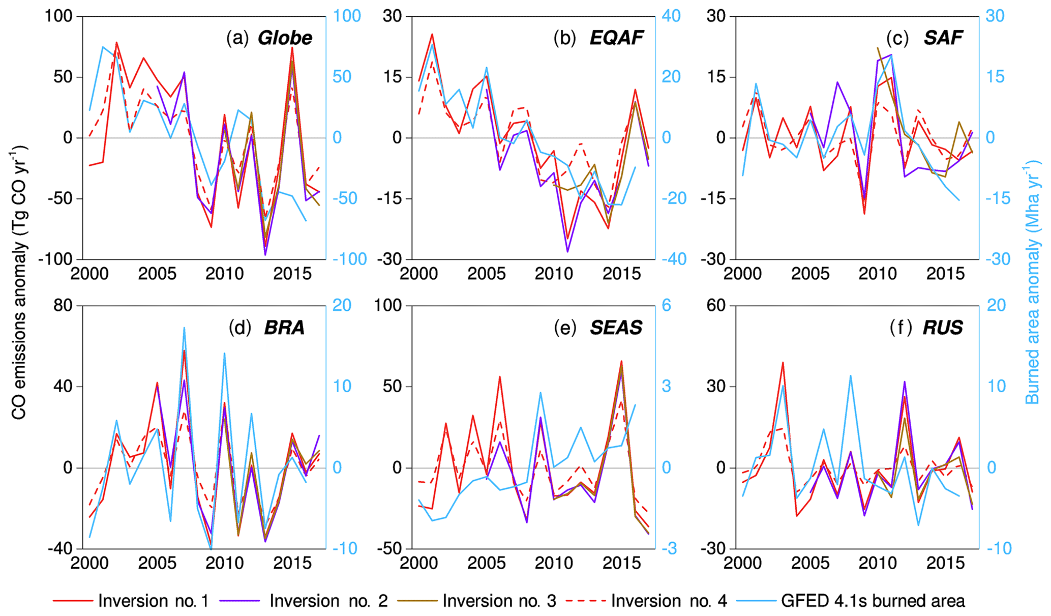
Figure 9Comparison of inversion-based biomass burning CO emission anomalies with GFED 4.1s burned area. The global total (a) and the top five emitters of biomass burning CO are presented here, including EQAF (b), SAF (c), BRA (d), SEAS (e), and RUS (f). We compare the regional emission anomalies estimated from Inversion nos. 1 to 4 to the GFED 4.1s burned area. We normalize burned area and emissions time series by removing the annual average to calculate the 2000–2017 anomalies, except that Inversion no. 2 and Inversion no. 3 subtract the 2000–2017 annual average emissions calculated from Inversion no. 1.
4.1 Influence of prior inter-annual variation
Inversion no. 4 has the same inversion setup as Inversion no. 1 except that it used the flat prior CO fluxes (seasonal climatology) without inter-annual variation. The prior CO fluxes used in Inversion no. 1 (Table S6) are composed of increasing anthropogenic emissions (0.33±0.14 % yr−1, p < 0.01) and decreasing but highly time-variable biomass burning emissions ( % yr−1, p=0.53), which lead to a slightly increasing global total source (0.16±0.18 % yr−1, p=0.07). Without this prior inter-annual variability, Inversion no. 4 estimates that the global CO source declined by % yr−1 (p < 0.01) and the global CO sink declined by % yr−1 (p < 0.01) during 2000–2017 (Table 3). The declining CO source can be decomposed into a relatively flat CO chemical production (0.03±0.09 % yr−1) and a rapidly declining surface emission ( % yr−1) that is primarily due to the decreasing anthropogenic ( % yr−1) and biomass burning ( % yr−1) emissions. Overall, Inversion no. 4 is highly consistent with Inversion no. 1 in regard to the relative trends in the anthropogenic (Table S7) and biomass burning (Table S10) sources globally (Fig. 6) and regionally (Fig. 7), especially for the top five emitters (Figs. 8, 9). This consistency suggests that the estimated declining trends in the global CO source and CO sink are not affected by the inter-annual variations of prior CO fluxes.
4.2 Drivers of declining CO emissions
We compare the inversion-based anthropogenic CO emissions to regional bottom-up inventories that are not used in our inversions (Fig. 8). Here we use the bottom-up inventory data from EPA for the USA (USEPA, 2018, Fig. 8a), from MEIC v1.3 for CHN (Zheng et al., 2018c, Fig. 8b), from TNO-MACC III for EU (Kuenen et al., 2014, Fig. 8c), from REAS v2.1 for SAS (Kurokawa et al., 2013, Fig. 8d), and from EDGAR v4.3.2 for EQAF (Crippa et al., 2018, Fig. 8e), while our prior inventory is the CEDS global inventory (see Sect. 2.2). These bottom-up emissions data are derived from detailed regional activity maps and sector-specific emission factors, except for EQAF, where we use the EDGAR v4.3.2 global inventory (up to 2012) due to the lack of regional inventories there. Figure 8 shows consistent anthropogenic CO emission trends between bottom-up and top-down estimates in all five regions, indicating that the inversion results capture the inter-annual variation of anthropogenic CO emissions well. The sectoral detail of bottom-up data allows us to identify the driving source sector in each region. The transport sector dominates the rapidly decreasing emissions in the USA and EU, while the industrial and residential sectors have driven down the emissions in CHN after 2005. The road transport, industrial, and residential sources all pushed up emissions in SAS during 2000–2010, while the growing residential source is mainly responsible for the continuous rising emissions in EQAF.
Distinct emission driver sectors reflect different stages of socio-economic development, fuel use, and emission regulation policies in different regions. Developed economies such as the USA and EU have improved their industrial and residential combustion facilities that now burn relatively clean energy at high combustion efficiencies. The transport sector accounts for the majority of the current emissions, and the progressive pollution control on vehicles has successfully cut CO emissions in the USA (Jiang et al., 2018) and EU (Crippa et al., 2016). CHN and SAS are both in the process of rapid industrialization and urbanization, which made their anthropogenic CO emissions rise up rapidly since 2000, driven by all the source sectors, especially the industrial and residential sources. To save energy and reduce air pollution, China has improved the combustion efficiency and strengthened the end-of-pipe pollution control since 2005, which has successfully cut industrial and residential CO emissions (Zheng et al., 2018a, c). China has also implemented stringent vehicle emission standards; however, the explosive growth in vehicle sales and oil use partly offsets the impact of vehicle pollution control, making the transport sector contribute less to emission reductions. The emissions from SAS are estimated to have increased up to 2010 and have remained flat since then, while the cause of flattening emissions is not very clear due to lack of bottom-up inventories for recent years. The underdeveloped economies in the EQAF have few emissions from the industrial and transport sources, and most of the emissions increase is driven by the growing residential source mainly for cooking and heating.
Biomass burning emissions are determined by burned area, fuel combustion rate per unit area, and emission factors per unit mass of fuel burned (van der Werf et al., 2017). Our inversion-based biomass burning CO emissions broadly follow the trends of GFED 4.1s burned area that is derived from satellite observations during 2000–2017 (Fig. 9), which suggests that burned area is the primary driver of biomass burning emissions variation. The global burned area is observed to have declined since 2000 (Fig. 9a) with the largest decline in the grassland and savanna ecosystems over EQAF (Fig. 9b). This declining trend is primarily driven by agricultural expansion and intensification, with more fire management and suppression due to population increase and socioeconomic development (Andela and van der Werf, 2014; Andela et al., 2017). Although extreme drought years could shortly expand the burned area, the overall downward trends in global burned area are robust due to the strong inverse relationship between fire activities and economic development (Andela et al., 2017). We have also noticed that the variations in burned area and biomass burning emissions did not have perfect matches in some years (e.g., the year of 2015). The mismatch can be explained by the inter-annual variation of fuel combustion rate and emission factors that mostly depend on burning conditions, land cover, and fuel type. For example, the 2015–2016 El Niño event caused severe fires on the drained peatlands in Indonesia that are not burned in normal years. This caused only a moderate increase in burned area but released a disproportionately large amount of CO because the peat fire emission factor is 210 g CO kg−1 dry matter (van der Werf et al., 2017), 3.3 times higher than that of savanna fires (63 g CO kg−1 dry matter) that regularly burn every year and contribute roughly half of the global biomass burning CO emissions.
4.3 Interactions between OH and CO
The global CO budget is affected by the interactions between OH and CO. A lower OH level translates into a proportionally smaller CO sink and thus estimates a smaller CO total source to achieve the source–sink balance (Müller et al., 2018). As such, the inter-annual variability of OH (if any) perturbs the long-term trends of the global CO budget. There are similar discussions for CH4 that a combination of declining OH and slightly growing CH4 source may explain the renewed growth of CH4 concentrations since 2007 (Rigby et al., 2017; Turner et al., 2017); otherwise, an abrupt increase in CH4 emissions since 2007 has to be assumed to match the CH4 observations (Turner et al., 2017). On the other hand, the declining CO burden in the atmosphere can leave more OH available to oxidize CH4 through the coupling of CO–OH–CH4, which means that the declining CO can stimulate the growth of CO chemical production (Gaubert et al., 2017). These interactions between OH and CO help understand the uncertainties induced by OH in our inversion results.
The tropospheric OH mean derived from Inversion no. 1 is 9.9×10⁵ molec. cm−3 and Inversion nos. 2 and 3 both give a mean OH of 10.0×10⁵ molec. cm−3. These values are close to the TransCom prior with less than 1 % difference (the prior uncertainty is 5 %). This is a medium level compared to the modeled OH of 6.5×10⁵ to 13.4×10⁵ molec. cm−3 in the Atmospheric Chemistry and Climate Model Intercomparison Project (ACCMIP) simulations (Voulgarakis et al., 2013). The three inversions all estimate a small inter-annual variation in OH, less than 2 % (Fig. S10). Inversion no. 1 that constrains OH through CO and MCF gives a small positive trend in OH during 2000–2008 (0.21±0.14 % yr−1, P < 0.01) and a small negative trend during 2008–2017 ( % yr−1, P=0.02). Inversion nos. 2 and 3 both estimate slightly increasing OH with the trends of 0.26±0.25 % yr−1 (P=0.05) and 0.19±0.21 % yr−1 (P=0.06), respectively, during their overlapping period 2010–2017. The estimated growing OH trends are larger than the downward trends estimated by Inversion no. 1. As Inversion nos. 2 and 3 additionally assimilate HCHO and CH4 that also react with OH, these results suggest that HCHO and CH4 tend to have a stronger constraint on the OH level than CO and MCF assimilated in Inversion no. 1. It should be noted that the mixing ratios of MCF in the atmosphere are approaching zero and therefore hardly constrain OH any more (Liang et al., 2017).
The debate on OH variation is still ongoing (Turner et al., 2019; Nisbet et al., 2019). OH was thought to be well buffered in the atmosphere, which means that OH is not sensitive to the variations of anthropogenic and natural emissions. This is reflected in the results of global chemistry and climate models (Naik et al., 2013; Voulgarakis et al., 2013). A recent 3-D inverse modeling by McNorton et al. (2018) also gave a small inter-annual variation of 1.8±0.4 % in the tropospheric OH from 2007 to 2015, broadly consistent with our inversion results (Fig. S10). In contrast, some two-box model inversions give larger inter-annual variations of about 5 %–8 % in the global OH mean (Rigby et al., 2017; Turner et al., 2017; Naus et al., 2019, Fig. S10). Rigby et al. (2017) and Turner et al. (2017) primarily used MCF to infer OH, and they both estimated declining OH from 2004/2005 to 2014/2013. This declining trend is not revealed by 3-D modeling studies, including our inversions here. Turner et al. (2017) also suggested slightly increasing OH since 2013, which agrees with our estimates of Inversion nos. 2 and 3. However, it should be noted that the uncertainty ranges assessed by those two-box model studies are larger than their estimated OH variations. Our 3-D inversions further suggest that the OH trend is sensitive to the observation constraints used. All these features suggest that the OH inter-annual variation is still underdetermined (Rigby et al., 2017; Turner et al., 2017).
The ability to simulate the nonlinear chemistry of OH is still weak in global models, which is another challenge to understand the OH variation. The LMDz-SACS model adopts a linearized chemical scheme to simulate the hydrocarbon reactions including CH4+OH, HCHO+OH, CO+OH, and MCF+OH. The nonlinear dynamics of the OH chemistry, such as the secondary OH production (Lelieveld et al., 2016) and the interaction of OH with the NOx chemistry (Miyazaki et al., 2017), is not represented. The negligible computational cost of this configuration for OH motivates it, but we also expect the optimization of OH through the joint assimilation of CH4, HCHO, CO, and MCF observations to counterbalance the simplicity of the scheme. Alternatively, it would be interesting to sophisticate the scheme by introducing key tracers in the OH chemistry (e.g., tropospheric ozone, NO, and NMVOCs) in the scheme together with prescribed (though uncertain) reaction rates, but we currently lack enough observations to constrain this additional complexity.
The OH trends derived from our inversions may be ambiguous, but we can still speculate that our main conclusion is robust to the possibly larger variation of OH. If a strong downward OH trend existed as two-box model studies suggested, we could see faster decreases in both global atmospheric CO sink and global atmospheric CO source than our current estimates. Although decreasing rates may be varied, the overall trends and drivers of the estimated global CO budget are not changed.

Figure 10Comparison of Inversion nos. 1, 2, and 3 with previous top-down estimates of the global CO budget. The comparison is conducted for the global CO source (a), the global CO sink (b), the surface direct emissions (c), the anthropogenic emissions (d), the biomass burning emissions (e), the CO chemical production (f), the CO production from CH4 oxidation (g), and the CO production from NMVOC oxidation (h).
4.4 Comparison with previous top-down estimates
We compile the top-down estimated global CO budget from 12 papers (Table S4) to compare with our inversion results. Compared to the nine studies using different inversion systems (Fig. 10), our inversion system is the only one with the capability of multi-species constraints and also the only one using MOPITT v7 data to constrain CO, while the previous studies had to use older versions of MOPITT data.
All these top-down studies converge on the estimates of global CO sources (Fig. 10a) but disagree on the split between surface emissions and chemical production, and also on the proportions of CH4-based and NMVOC-based CO productions. For example, Jiang et al. (2017) estimated consistent declining trends in anthropogenic (Fig. 10d) and biomass burning (Fig. 10e) CO emissions as our estimates, but their annual average emissions are 20 %–37 % lower than our results. The CO production from NMVOCs shows a large spread (Fig. 10h) among different inversion studies. Gaubert et al. (2017) estimated a CO chemical production quite close to our estimates (Fig. 10f), while they gave lower CH4 oxidation and higher NMVOC oxidation. The biogenic and oceanic CO emissions derived from different inversions are 100–200 and 20 Tg CO yr−1 (Table S4), respectively, which is consistent with our estimates (Table 3). Few studies estimated the global CO sink (Fig. 10b), except Gaubert et al. (2017), who gave a declining CO sink from 2002 to 2013 that agrees with our estimates, but the Gaubert et al. (2017) values are 15 % lower on average.
The other three inversions in the comparison are all derived from previous versions of our inversion system with multi-species constraints (Fortems-Cheiney et al., 2011, 2012; Yin et al., 2015). Compared to these previous estimates (Fig. S11), we have increased the spatial resolution of our transport model, used improved prior data, and assimilated the new MOPITT v7 observations. Therefore, the updated inversion results in this paper are expected to have better quality, leading to updated trend estimates of the global CO source (Fig. S11a), CO sink (Fig. S11b), surface CO emissions (Fig. S11c), and CO production from NMVOCs (Fig. S11h).
The data we use as an input of our inversion models and their references are as follows. The MOPITT v7 TIR-NIR product (Deeter et al., 2017) for 2000–2017 can be downloaded from https://l0dup05.larc.nasa.gov/opendap/MOPITT/MOP02J.007/ (Ziskin, 2016). The OMI v3 HCHO column retrievals (González Abad et al., 2015) for 2004–2017 can be downloaded from https://aura.gesdisc.eosdis.nasa.gov/data/Aura_OMI_Level2/OMHCHO.003/ (Chance, 2007). The GOSAT XCH4 retrievals produced by the University of Leicester (Parker et al., 2011) for 2009–2017 can be downloaded from http://www.leos.le.ac.uk/data/GHG/GOSAT/v7.2/CH4_GOS_OCPR_v7.2.tar.gz (Parker, 2018). The ground-based observations from WDCGG can be downloaded from https://gaw.kishou.go.jp/ (last access: 10 September 2019), and those from TCCON (Wunch et al., 2011) can be downloaded from https://tccondata.org/ (a reference for each TCCON site can be found in Fig. A1). The CEDS emissions data can be downloaded from http://www.globalchange.umd.edu/ceds/ceds-cmip6-data/ (Hoesly et al., 2018). The GFED emissions data can be downloaded from https://www.globalfiredata.org/ (van der Werf et al., 2017).
The global CO budget during 2000–2017 derived from Inversion nos. 1, 2, and 3 in this study can be downloaded from https://doi.org/10.6084/m9.figshare.c.4454453.v1 (Zheng et al., 2019). These are monthly gridded data products at the spatial resolution of 3.75∘ longitude ×1.9∘ latitude, including surface CO emissions from different source sectors (i.e., anthropogenic, biomass burning, biogenic, and oceanic), CO chemical production, and CO chemical sinks.
We have estimated the global atmospheric CO budget during 2000–2017 through a multi-species atmospheric inversion system and have investigated its magnitude, variation, and drivers to understand the observed steady decline in the atmospheric CO burdens. The inversion-based CO budget significantly improves the modeled CO concentrations and trends compared with independent ground-based observations from the WDCGG and TCCON archives. The inversion results attribute the drivers of the declining MOPITT CO columns during 2000–2017 to a decrease in anthropogenic and biomass burning CO emissions that more than offsets the growing CO chemical production in the atmosphere. The decline in anthropogenic CO emissions mainly occurs in the US, Europe, and China, highly consistent with state-of-the-art regional bottom-up inventories, which show that the transport sector drives emissions down in the US and Europe, and the improved combustion efficiency and pollution control in the industrial and residential sources are major drivers in China. The declining biomass burning emissions are consistent with the overall downward trends of satellite-based global burned areas, which is the consequence of agricultural and economic expansion as reported in other published studies. Nonetheless, biomass burning still has significant inter-annual variability and releases a large amount of CO in extreme drought years. We have investigated the robustness and uncertainties of the inversion results through three inversion analyses and one sensitivity inversion test, from which we demonstrated that the overall declining trends in global and regional CO sources and the underlying drivers are robust to different observation constraints, to prior inter-annual variation, and to possible OH trends. Additionally, our inversion results include emission estimates for methane and formaldehyde that will be the topic of a future dedicated evaluation.
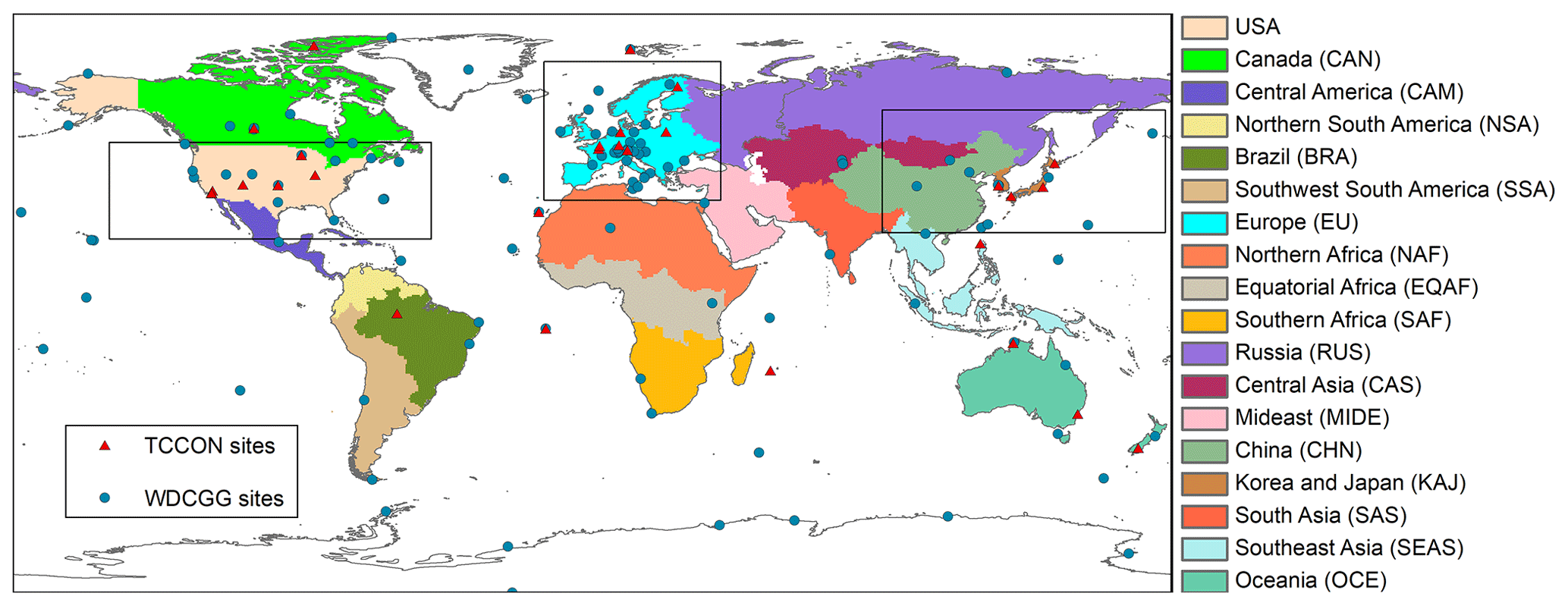
Figure A1The 18 regions used in this study. The WDCGG (blue dot) and TCCON (red triangle) sites are located on the map. The three black boxes select the WDCGG sites used in the model evaluation for the US, Europe, and China, respectively, in Figs. S7, S8, and S9. The TCCON stations include Indianapolis (Iraci et al., 2017a), Manaus (Dubey et al., 2017a), Sodankylä (Kivi et al., 2017), Lauder (Sherlock et al., 2017a, b), Burgos (Morino et al., 2018), Ascension Island (Feist et al., 2017), Réunion (De Mazière et al., 2017), Caltech (Wennberg et al., 2017a), Zugspitze (Sussmann and Rettinger, 2018), Ny Ålesund (Notholt et al., 2017a), Orléans (Warneke et al., 2017), Jet Propulsion Laboratory (Wennberg et al., 2017b, c), Saga (Kawakami et al., 2017), Izana (Blumenstock et al., 2017), Edwards (Iraci et al., 2017b), Garmisch (Sussmann and Rettinger, 2017), Bremen (Notholt et al., 2017b), Karlsruhe (Hase et al., 2017), Four Corners (Dubey et al., 2017b), Wollongong (Griffith et al., 2017a), East Trout Lake (Wunch et al., 2017), Paris (Té et al., 2017), Anmeyondo (Goo et al., 2017), Park Falls (Wennberg et al., 2017d), Lamont (Wennberg et al., 2017e), Bialystok (Deutscher et al., 2017), Rikubetsu (Morino et al., 2017a), Eureka (Strong et al., 2018), Tsukuba (Morino et al., 2017b), and Darwin (Griffith et al., 2017b).
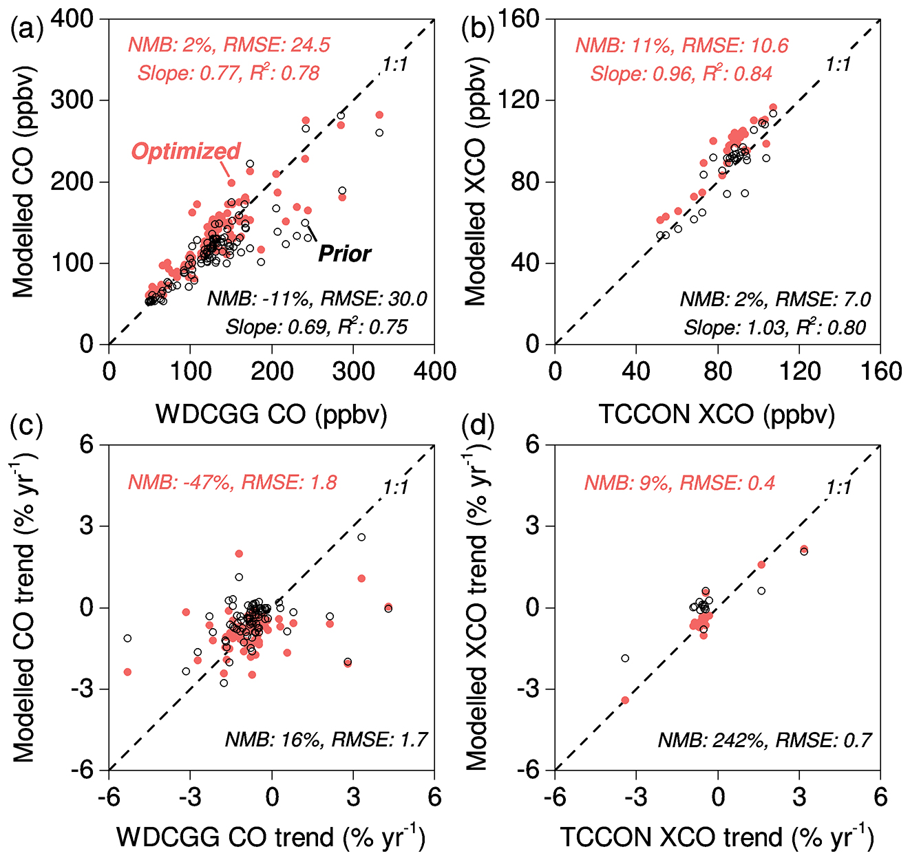
Figure B1Evaluation of Inversion no. 1 with independent ground-based observations. Annual average surface CO concentrations and XCO modeled by both prior (black dot) and optimized (red dot) emissions are compared with ground-based observations from the WDCGG (a) and TCCON networks (b), respectively. The 2000–2017 trends that are significant in a statistical test (p < 0.05) observed by WDCGG (c) and TCCON (d) are used to evaluate the modeled trends. The trends are calculated based on monthly time series using a curve fitting method as described in Zheng et al. (2018a).
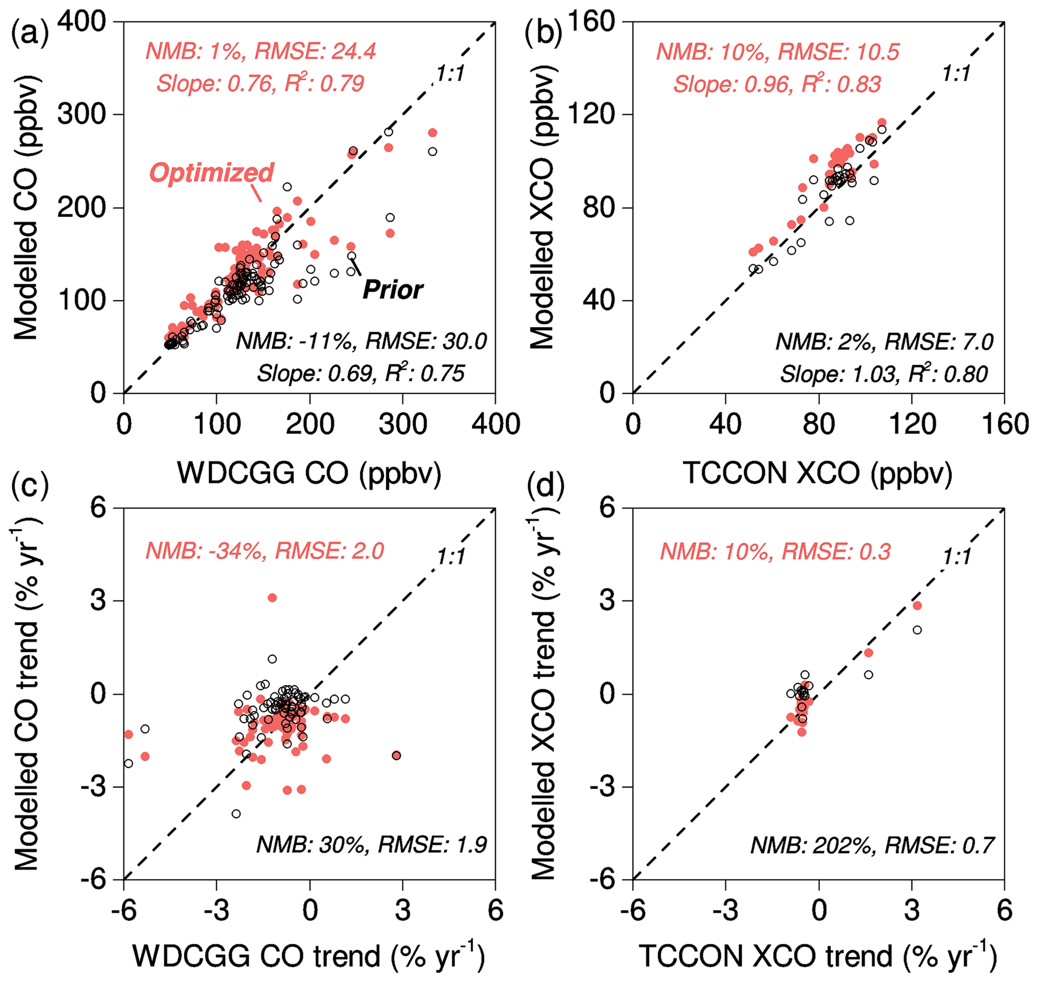
Figure B2Evaluation of Inversion no. 2 with independent ground-based observations. Annual average surface CO concentrations and XCO modeled by both prior (black dot) and optimized (red dot) emissions are compared with ground-based observations from the WDCGG (a) and TCCON networks (b), respectively. The 2005–2017 trends that are significant in a statistical test (p < 0.05) observed by WDCGG (c) and TCCON (d) are used to evaluate the modeled trends. The trends are calculated based on monthly time series using a curve fitting method as described in Zheng et al. (2018a).
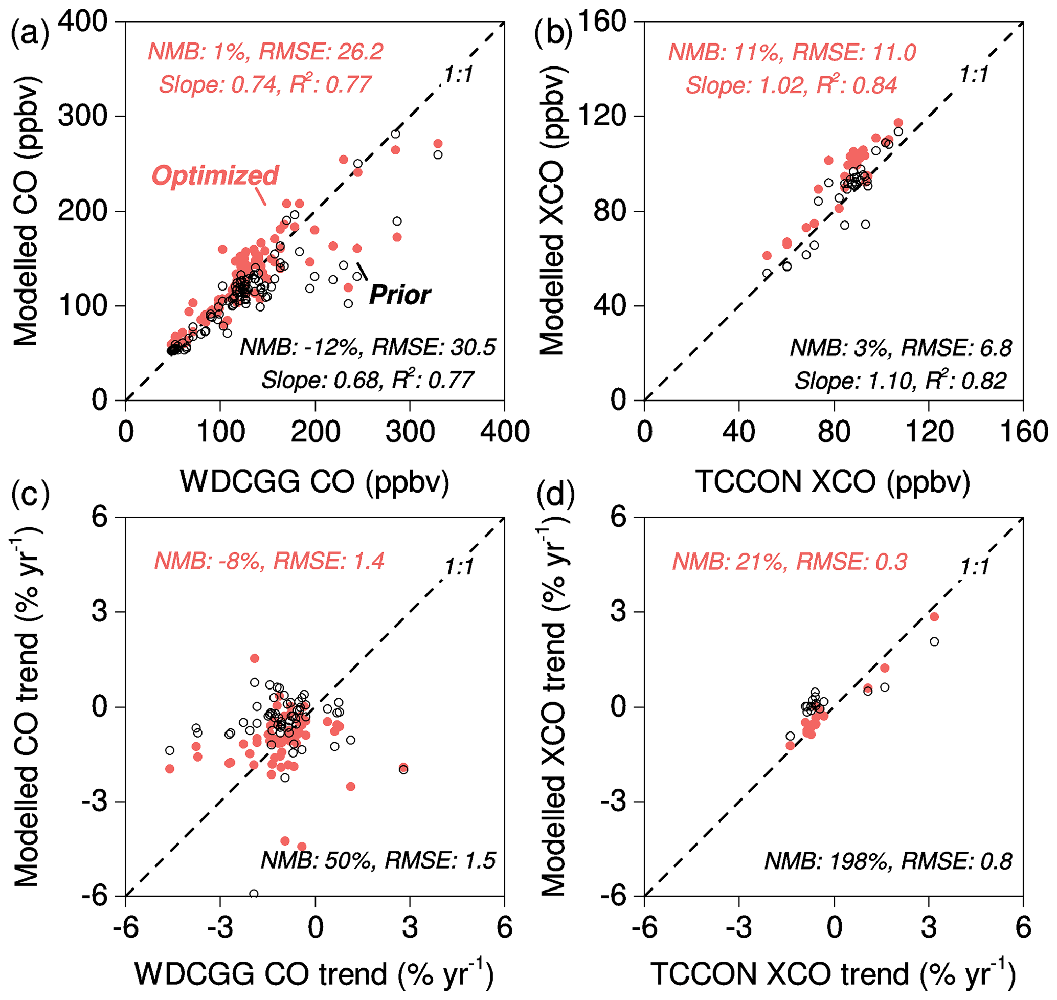
Figure B3Evaluation of Inversion no. 3 with independent ground-based observations. Annual average surface CO concentrations and XCO modeled by both prior (black dot) and optimized (red dot) emissions are compared with ground-based observations from the WDCGG (a) and TCCON networks (b), respectively. The 2010–2017 trends that are significant in a statistical test (p < 0.05) observed by WDCGG (c) and TCCON (d) are used to evaluate the modeled trends. The trends are calculated based on monthly time series using a curve fitting method as described in Zheng et al. (2018a).
The supplement related to this article is available online at: https://doi.org/10.5194/essd-11-1411-2019-supplement.
BZ, FC, and PC designed the study. BZ performed the inversion analysis of the global CO budget and created the data product. The manuscript was written by BZ and revised and discussed by all the coauthors.
The authors declare that they have no conflict of interest.
We acknowledge the NCAR MOPITT group for the production of the CO retrievals and the Goddard Earth Sciences Data and Information Services Center for the production of the SAO OMI HCHO retrievals. We thank the WDCGG and TCCON archives for publishing the ground-based CO observations, and we are grateful to all the people involved in maintaining the network and archiving the observation data. We also thank Francois Marabelle for computing support at LSCE. The GOSAT XCH4 retrievals are processed using the ALICE High Performance Computing Facility at the University of Leicester.
This work benefited from HPC resources from GENCI-TGCC (grant no. 2018-A0050102201). Robert J. Parker is funded via the UK National Centre for Earth Observation (NCEO grant no. nceo020005).
This paper was edited by Thomas Blunier and reviewed by three anonymous referees.
Ahmadov, R., Gerbig, C., Kretschmer, R., Koerner, S., Neininger, B., Dolman, A. J., and Sarrat, C.: Mesoscale covariance of transport and CO2 fluxes: Evidence from observations and simulations using the WRF-VPRM coupled atmosphere-biosphere model, J. Geophys. Res.-Atmos., 112, D22107, https://doi.org/10.1029/2007JD008552, 2007.
Andela, N. and van der Werf, G. R.: Recent trends in African fires driven by cropland expansion and El Niño to La Niña transition, Nat. Clim. Change, 4, 791–795, https://doi.org/10.1038/nclimate2313, 2014.
Andela, N., Morton, D. C., Giglio, L., Chen, Y., van der Werf, G. R., Kasibhatla, P. S., DeFries, R. S., Collatz, G. J., Hantson, S., Kloster, S., Bachelet, D., Forrest, M., Lasslop, G., Li, F., Mangeon, S., Melton, J. R., Yue, C., and Randerson, J. T.: A human-driven decline in global burned area, Science, 356, 1356–1362, https://doi.org/10.1126/science.aal4108, 2017.
Arellano, A. F., Kasibhatla, P. S., Giglio, L., van der Werf, G. R., Randerson, J. T., and Collatz, G. J.: Time-dependent inversion estimates of global biomass-burning CO emissions using Measurement of Pollution in the Troposphere (MOPITT) measurements, J. Geophys. Res.-Atmos., 111, D09303, https://doi.org/10.1029/2005JD006613, 2006.
Arellano Jr., A. F., Kasibhatla, P. S., Giglio, L., van der Werf, G. R., and Randerson, J. T.: Top-down estimates of global CO sources using MOPITT measurements, Geophys. Res. Lett., 31, L01104, https://doi.org/10.1029/2003GL018609, 2004.
Bloom, A. A., Bowman, K. W., Lee, M., Turner, A. J., Schroeder, R., Worden, J. R., Weidner, R., McDonald, K. C., and Jacob, D. J.: A global wetland methane emissions and uncertainty dataset for atmospheric chemical transport models (WetCHARTs version 1.0), Geosci. Model Dev., 10, 2141–2156, https://doi.org/10.5194/gmd-10-2141-2017, 2017.
Blumenstock, T., Hase, F., Schneider, M., García, O. E., and Sepúlveda, E.: TCCON data from Izana (ES), Release GGG2014.R1, https://doi.org/10.14291/tccon.ggg2014.izana01.r1, 2017.
Bruhn, D., Albert, K. R., Mikkelsen, T. N., and Ambus, P.: UV-induced carbon monoxide emission from living vegetation, Biogeosciences, 10, 7877–7882, https://doi.org/10.5194/bg-10-7877-2013, 2013.
Canadian National Fire Database: available at: http://cwfis.cfs.nrcan.gc.ca/ha/nfdb (last access: 16 January 2019), 2018.
Conte, L., Szopa, S., Séférian, R., and Bopp, L.: The oceanic cycle of carbon monoxide and its emissions to the atmosphere, Biogeosciences, 16, 881–902, https://doi.org/10.5194/bg-16-881-2019, 2019.
Chance, K.: OMI/Aura Formaldehyde (HCHO) Total Column 1-orbit L2 Swath 13×24 km V003, NASA Goddard Earth Sciences Data and Information Services Center (GES DISC), https://doi.org/10.5067/aura/omi/data2015, 2007 (data available at: https://aura.gesdisc.eosdis.nasa.gov/data/Aura_OMI_Level2/OMHCHO.003/, last access: 10 September 2019).
Chen, Y., Morton, D. C., Andela, N., van der Werf, G. R., Giglio, L., and Randerson, J. T.: A pan-tropical cascade of fire driven by El Niño/Southern Oscillation, Nat. Clim. Change, 7, 906–911, https://doi.org/10.1038/s41558-017-0014-8, 2017.
Chevallier, F., Fisher, M., Peylin, P., Serrar, S., Bousquet, P., Bréon, F. M., Chédin, A., and Ciais, P.: Inferring CO2 sources and sinks from satellite observations: Method and application to TOVS data, J. Geophys. Res.-Atmos., 110, D24309, https://doi.org/10.1029/2005JD006390, 2005.
Chevallier, F., Fortems, A., Bousquet, P., Pison, I., Szopa, S., Devaux, M., and Hauglustaine, D. A.: African CO emissions between years 2000 and 2006 as estimated from MOPITT observations, Biogeosciences, 6, 103–111, https://doi.org/10.5194/bg-6-103-2009, 2009.
Crippa, M., Janssens-Maenhout, G., Dentener, F., Guizzardi, D., Sindelarova, K., Muntean, M., Van Dingenen, R., and Granier, C.: Forty years of improvements in European air quality: regional policy-industry interactions with global impacts, Atmos. Chem. Phys., 16, 3825–3841, https://doi.org/10.5194/acp-16-3825-2016, 2016.
Crippa, M., Guizzardi, D., Muntean, M., Schaaf, E., Dentener, F., van Aardenne, J. A., Monni, S., Doering, U., Olivier, J. G. J., Pagliari, V., and Janssens-Maenhout, G.: Gridded emissions of air pollutants for the period 1970–2012 within EDGAR v4.3.2, Earth Syst. Sci. Data, 10, 1987–2013, https://doi.org/10.5194/essd-10-1987-2018, 2018.
Dee, D. P., Uppala, S. M., Simmons, A. J., Berrisford, P., Poli, P., Kobayashi, S., Andrae, U., Balmaseda, M. A., Balsamo, G., Bauer, P., Bechtold, P., Beljaars, A. C. M., van de Berg, L., Bidlot, J., Bormann, N., Delsol, C., Dragani, R., Fuentes, M., Geer, A. J., Haimberger, L., Healy, S. B., Hersbach, H., Hólm, E. V., Isaksen, L., Kållberg, P., Köhler, M., Matricardi, M., McNally, A. P., Monge-Sanz, B. M., Morcrette, J. J., Park, B. K., Peubey, C., de Rosnay, P., Tavolato, C., Thépaut, J. N., and Vitart, F.: The ERA-Interim reanalysis: configuration and performance of the data assimilation system, Q. J. Roy. Meteorol. Soc., 137, 553–597, https://doi.org/10.1002/qj.828, 2011.
Deeter, M. N., Edwards, D. P., Francis, G. L., Gille, J. C., Martínez-Alonso, S., Worden, H. M., and Sweeney, C.: A climate-scale satellite record for carbon monoxide: the MOPITT Version 7 product, Atmos. Meas. Tech., 10, 2533–2555, https://doi.org/10.5194/amt-10-2533-2017, 2017.
De Mazière, M., Sha, M. K., Desmet, F., Hermans, C., Scolas, F., Kumps, N., Metzger, J.-M., Duflot, V., and Cammas, J.-P.: TCCON data from Réunion Island (RE), Release GGG2014.R1, https://doi.org/10.14291/tccon.ggg2014.reunion01.r1, 2017.
De Smedt, I., Stavrakou, T., Müller, J.-F., van der A, R. J., and Van Roozendael, M.: Trend detection in satellite observations of formaldehyde tropospheric columns, Geophys. Res. Lett., 37, L18808, https://doi.org/10.1029/2010GL044245, 2010.
Deutscher, N. M., Notholt, J., Messerschmidt, J., Weinzierl, C., Warneke, T., Petri, C., and Grupe, P.: TCCON data from Bialystok (PL), Release GGG2014.R1, https://doi.org/10.14291/tccon.ggg2014.bialystok01.r1/1183984, 2017.
Dubey, M. K., Henderson, B. G., Green, D., Butterfield, Z. T., Keppel-Aleks, G., Allen, N. T., Blavier, J.-F., Roehl, C. M., Wunch, D., and Lindenmaier, R.: TCCON data from Manaus (BR), Release GGG2014.R0, https://doi.org/10.14291/tccon.ggg2014.manaus01.r0/1149274, 2017a.
Dubey, M. K., Lindenmaier, R., Henderson, B. G., Green, D., Allen, N. T., Roehl, C. M., Blavier, J.-F., Butterfield, Z. T., Love, S., Hamelmann, J. D., and Wunch, D.: TCCON data from Four Corners (US), Release GGG2014.R0, https://doi.org/10.14291/tccon.ggg2014.fourcorners01.r0/1149272, 2017b.
Duncan, B. N., Logan, J. A., Bey, I., Megretskaia, I. A., Yantosca, R. M., Novelli, P. C., Jones, N. B., and Rinsland, C. P.: Global budget of CO, 1988–1997: Source estimates and validation with a global model, J. Geophys. Res.-Atmos., 112, D22301, https://doi.org/10.1029/2007JD008459, 2007.
Feist, D. G., Arnold, S. G., John, N., and Geibel, M. C.: TCCON data from Ascension Island (SH), Release GGG2014.R0, https://doi.org/10.14291/tccon.ggg2014.ascension01.r0/1149285, 2017.
Folberth, G. A., Hauglustaine, D. A., Lathière, J., and Brocheton, F.: Interactive chemistry in the Laboratoire de Météorologie Dynamique general circulation model: model description and impact analysis of biogenic hydrocarbons on tropospheric chemistry, Atmos. Chem. Phys., 6, 2273–2319, https://doi.org/10.5194/acp-6-2273-2006, 2006.
Fortems-Cheiney, A., Chevallier, F., Pison, I., Bousquet, P., Szopa, S., Deeter, M. N., and Clerbaux, C.: Ten years of CO emissions as seen from Measurements of Pollution in the Troposphere (MOPITT), J. Geophys. Res.-Atmos., 116, D05304, https://doi.org/10.1029/2010JD014416, 2011.
Fortems-Cheiney, A., Chevallier, F., Pison, I., Bousquet, P., Saunois, M., Szopa, S., Cressot, C., Kurosu, T. P., Chance, K., and Fried, A.: The formaldehyde budget as seen by a global-scale multi-constraint and multi-species inversion system, Atmos. Chem. Phys., 12, 6699–6721, https://doi.org/10.5194/acp-12-6699-2012, 2012.
Gaubert, B., Worden, H. M., Arellano, A. F. J., Emmons, L. K., Tilmes, S., Barré, J., Martinez Alonso, S., Vitt, F., Anderson, J. L., Alkemade, F., Houweling, S., and Edwards, D. P.: Chemical Feedback From Decreasing Carbon Monoxide Emissions, Geophys. Res. Lett., 44, 9985–9995, https://doi.org/10.1002/2017GL074987, 2017.
Gilbert, J. C. and Lemaréchal, C.: Some numerical experiments with variable-storage quasi-Newton algorithms, Math. Program., 45, 407–435, https://doi.org/10.1007/bf01589113, 1989.
González Abad, G., Liu, X., Chance, K., Wang, H., Kurosu, T. P., and Suleiman, R.: Updated Smithsonian Astrophysical Observatory Ozone Monitoring Instrument (SAO OMI) formaldehyde retrieval, Atmos. Meas. Tech., 8, 19–32, https://doi.org/10.5194/amt-8-19-2015, 2015.
Granier, C., Bessagnet, B., Bond, T., D'Angiola, A., Denier van der Gon, H., Frost, G. J., Heil, A., Kaiser, J. W., Kinne, S., Klimont, Z., Kloster, S., Lamarque, J.-F., Liousse, C., Masui, T., Meleux, F., Mieville, A., Ohara, T., Raut, J.-C., Riahi, K., Schultz, M. G., Smith, S. J., Thompson, A., van Aardenne, J., van der Werf, G. R., and van Vuuren, D. P.: Evolution of anthropogenic and biomass burning emissions of air pollutants at global and regional scales during the 1980–2010 period, Climatic Chang., 109, 163–190, https://doi.org/10.1007/s10584-011-0154-1, 2011.
Gratz, L. E., Jaffe, D. A., and Hee, J. R.: Causes of increasing ozone and decreasing carbon monoxide in springtime at the Mt. Bachelor Observatory from 2004 to 2013, Atmos. Environ., 109, 323–330, https://doi.org/10.1016/j.atmosenv.2014.05.076, 2015.
Goo, T.-Y., Oh, Y.-S., and Velazco, V. A.: TCCON data from Anmeyondo (KR), Release GGG2014.R0, https://doi.org/10.14291/tccon.ggg2014.anmeyondo01.r0/1149284, 2017.
Griffith, D. W. T., Velazco, V. A., Deutscher, N. M., Paton-Walsh, C., Jones, N. B., Wilson, S. R., Macatangay, R. C., Kettlewell, G. C., Buchholz, R. R., and Riggenbach, M. O.: TCCON data from Wollongong (AU), Release GGG2014.R0, https://doi.org/10.14291/tccon.ggg2014.wollongong01.r0/1149291, 2017a.
Griffith, D. W. T., Deutscher, N. M., Velazco, V. A., Wennberg, P. O., Yavin, Y., Keppel-Aleks, G., Washenfelder, R. A., Toon, G. C., Blavier, J.-F., Paton-Walsh, C., Jones, N. B., Kettlewell, G. C., Connor, B. J., Macatangay, R. C., Roehl, C., Ryczek, M., Glowacki, J., Culgan, T., and Bryant, G. W.: TCCON data from Darwin (AU), Release GGG2014.R0, https://doi.org/10.14291/tccon.ggg2014.darwin01.r0/1149290, 2017b.
Hase, F., Blumenstock, T., Dohe, S., Groß, J., and Kiel, M.: TCCON data from Karlsruhe (DE), Release GGG2014.R1, https://doi.org/10.14291/tccon.ggg2014.karlsruhe01.r1/1182416, 2017.
Hoesly, R. M., Smith, S. J., Feng, L., Klimont, Z., Janssens-Maenhout, G., Pitkanen, T., Seibert, J. J., Vu, L., Andres, R. J., Bolt, R. M., Bond, T. C., Dawidowski, L., Kholod, N., Kurokawa, J.-I., Li, M., Liu, L., Lu, Z., Moura, M. C. P., O'Rourke, P. R., and Zhang, Q.: Historical (1750–2014) anthropogenic emissions of reactive gases and aerosols from the Community Emissions Data System (CEDS), Geosci. Model Dev., 11, 369–408, https://doi.org/10.5194/gmd-11-369-2018, 2018 (data available at: http://www.globalchange.umd.edu/ceds/ceds-cmip6-data/, last access: 10 September 2019).
Iraci, L. T., Podolske, J. R., Hillyard, P. W., Roehl, C., Wennberg, P. O., Blavier, J.-F., Landeros, J., Allen, N., Wunch, D., Zavaleta, J., Quigley, E., Osterman, G. B., Barrow, E., and Barney, J.: TCCON data from Indianapolis (US), Release GGG2014.R1, https://doi.org/10.14291/tccon.ggg2014.indianapolis01.r1/1330094, 2017a.
Iraci, L. T., Podolske, J. R., Hillyard, P. W., Roehl, C., Wennberg, P. O., Blavier, J.-F., Landeros, J., Allen, N., Wunch, D., Zavaleta, J., Quigley, E., Osterman, G. B., Albertson, R., Dunwoody, K., and Boyden, H.: TCCON data from Edwards (US), Release GGG2014.R1, https://doi.org/10.14291/tccon.ggg2014.edwards01.r1/1255068, 2017b.
Jiang, Z., Worden, J. R., Worden, H., Deeter, M., Jones, D. B. A., Arellano, A. F., and Henze, D. K.: A 15-year record of CO emissions constrained by MOPITT CO observations, Atmos. Chem. Phys., 17, 4565–4583, https://doi.org/10.5194/acp-17-4565-2017, 2017.
Jiang, Z., McDonald, B. C., Worden, H., Worden, J. R., Miyazaki, K., Qu, Z., Henze, D. K., Jones, D. B. A., Arellano, A. F., Fischer, E. V., Zhu, L., and Boersma, K. F.: Unexpected slowdown of US pollutant emission reduction in the past decade, P. Natl. Acad. Sci. USA, 115, 5099, https://doi.org/10.1073/pnas.1801191115, 2018.
Jiménez-Muñoz, J. C., Mattar, C., Barichivich, J., Santamaría-Artigas, A., Takahashi, K., Malhi, Y., Sobrino, J. A., and Schrier, G. v. d.: Record-breaking warming and extreme drought in the Amazon rainforest during the course of El Niño 2015–2016, Sci. Rep.-UK, 6, 33130, https://doi.org/10.1038/srep33130, 2016.
Kawakami, S., Ohyama, H., Arai, K., Okumura, H., Taura, C., Fukamachi, T., and Sakashita, M.: TCCON data from Saga (JP), Release GGG2014.R0, https://doi.org/10.14291/tccon.ggg2014.saga01.r0/1149283, 2017.
Khalil, M. A. K. and Rasmussen, R. A.: Global decrease in atmospheric carbon monoxide concentration, Nature, 370, 639–641, https://doi.org/10.1038/370639a0, 1994.
Kivi, R., Heikkinen, P., and Kyrö, E.: TCCON data from Sodankylä (FI), Release GGG2014.R0, https://doi.org/10.14291/tccon.ggg2014.sodankyla01.r0/1149280, 2017.
Kopacz, M., Jacob, D. J., Fisher, J. A., Logan, J. A., Zhang, L., Megretskaia, I. A., Yantosca, R. M., Singh, K., Henze, D. K., Burrows, J. P., Buchwitz, M., Khlystova, I., McMillan, W. W., Gille, J. C., Edwards, D. P., Eldering, A., Thouret, V., and Nedelec, P.: Global estimates of CO sources with high resolution by adjoint inversion of multiple satellite datasets (MOPITT, AIRS, SCIAMACHY, TES), Atmos. Chem. Phys., 10, 855–876, https://doi.org/10.5194/acp-10-855-2010, 2010.
Kuenen, J. J. P., Visschedijk, A. J. H., Jozwicka, M., and Denier van der Gon, H. A. C.: TNO-MACC_II emission inventory; a multi-year (2003–2009) consistent high-resolution European emission inventory for air quality modelling, Atmos. Chem. Phys., 14, 10963–10976, https://doi.org/10.5194/acp-14-10963-2014, 2014.
Kurokawa, J., Ohara, T., Morikawa, T., Hanayama, S., Janssens-Maenhout, G., Fukui, T., Kawashima, K., and Akimoto, H.: Emissions of air pollutants and greenhouse gases over Asian regions during 2000–2008: Regional Emission inventory in ASia (REAS) version 2, Atmos. Chem. Phys., 13, 11019–11058, https://doi.org/10.5194/acp-13-11019-2013, 2013.
Kuze, A., Suto, H., Nakajima, M., and Hamazaki, T.: Thermal and near infrared sensor for carbon observation Fourier-transform spectrometer on the Greenhouse Gases Observing Satellite for greenhouse gases monitoring, Appl. Opt., 48, 6716–6733, https://doi.org/10.1364/AO.48.006716, 2009.
Lelieveld, J., Gromov, S., Pozzer, A., and Taraborrelli, D.: Global tropospheric hydroxyl distribution, budget and reactivity, Atmos. Chem. Phys., 16, 12477–12493, https://doi.org/10.5194/acp-16-12477-2016, 2016.
Lewis, S. L., Brando, P. M., Phillips, O. L., van der Heijden, G. M. F., and Nepstad, D.: The 2010 Amazon Drought, Science, 331, 554–554, https://doi.org/10.1126/science.1200807, 2011.
Liang, Q., Chipperfield, M. P., Fleming, E. L., Abraham, N. L., Braesicke, P., Burkholder, J. B., Daniel, J. S., Dhomse, S., Fraser, P. J., Hardiman, S. C., Jackman, C. H., Kinnison, D. E., Krummel, P. B., Montzka, S. A., Morgenstern, O., McCulloch, A., Mühle, J., Newman, P. A., Orkin, V. L., Pitari, G., Prinn, R. G., Rigby, M., Rozanov, E., Stenke, A., Tummon, F., Velders, G. J. M., Visioni, D., and Weiss, R. F.: Deriving Global OH Abundance and Atmospheric Lifetimes for Long-Lived Gases: A Search for CH3CCl3 Alternatives, J. Geophys. Res.-Atmos., 122, 11914–11933, https://doi.org/10.1002/2017jd026926, 2017.
Liu, J., Bowman, K. W., Schimel, D. S., Parazoo, N. C., Jiang, Z., Lee, M., Bloom, A. A., Wunch, D., Frankenberg, C., Sun, Y., O'Dell, C. W., Gurney, K. R., Menemenlis, D., Gierach, M., Crisp, D., and Eldering, A.: Contrasting carbon cycle responses of the tropical continents to the 2015–2016 El Niño, Science, 358, eaam5690, https://doi.org/10.1126/science.aam5690, 2017.
McNorton, J., Wilson, C., Gloor, M., Parker, R. J., Boesch, H., Feng, W., Hossaini, R., and Chipperfield, M. P.: Attribution of recent increases in atmospheric methane through 3-D inverse modelling, Atmos. Chem. Phys., 18, 18149–18168, https://doi.org/10.5194/acp-18-18149-2018, 2018.
Miyazaki, K., Eskes, H., Sudo, K., Boersma, K. F., Bowman, K., and Kanaya, Y.: Decadal changes in global surface NOx emissions from multi-constituent satellite data assimilation, Atmos. Chem. Phys., 17, 807–837, https://doi.org/10.5194/acp-17-807-2017, 2017.
Montzka, S. A., Krol, M., Dlugokencky, E., Hall, B., Jöckel, P., and Lelieveld, J.: Small Interannual Variability of Global Atmospheric Hydroxyl, Science, 331, 67–69, https://doi.org/10.1126/science.1197640, 2011.
Morino, I., Yokozeki, N., Matsuzaki, T., and Horikawa, M.: TCCON data from Rikubetsu (JP), Release GGG2014.R2, https://doi.org/10.14291/tccon.ggg2014.rikubetsu01.r2, 2017a.
Morino, I., Matsuzaki, T., and Horikawa, M.: TCCON data from Tsukuba (JP), 125HR, Release GGG2014.R2, https://doi.org/10.14291/tccon.ggg2014.tsukuba02.r2, 2017b.
Morino, I., Velazco, V. A., Hori, A., Uchino, O., and Griffith, D. W. T.: TCCON data from Burgos, Ilocos Norte (PH), Release GGG2014.R0, https://doi.org/10.14291/tccon.ggg2014.burgos01.r0, 2018.
Müller, J.-F., Stavrakou, T., Bauwens, M., George, M., Hurtmans, D., Coheur, P.-F., Clerbaux, C., and Sweeney, C.: Top-Down CO Emissions Based On IASI Observations and Hemispheric Constraints on OH Levels, Geophys. Res. Lett., 45, 1621–1629, https://doi.org/10.1002/2017GL076697, 2018.
Myhre, G., Shindell, D., Bréon, F.-M., Collins, W., Fuglestvedt, J., Huang, J., Koch, D., Lamarque, J.-F., Lee, D., Mendoza, B., Nakajima, T., Robock, A., Stephens, G., Takemura, T., and Zhang, H.: Anthropogenic and natural radiative forcing, in: climate change 2013: the physical science basis Contribution of Working Group I to the Fifth Assessment Report of the Intergovernmental Panel on Climate Change, Cambridge, Cambridge University Press, 2013.
Naik, V., Voulgarakis, A., Fiore, A. M., Horowitz, L. W., Lamarque, J.-F., Lin, M., Prather, M. J., Young, P. J., Bergmann, D., Cameron-Smith, P. J., Cionni, I., Collins, W. J., Dalsøren, S. B., Doherty, R., Eyring, V., Faluvegi, G., Folberth, G. A., Josse, B., Lee, Y. H., MacKenzie, I. A., Nagashima, T., van Noije, T. P. C., Plummer, D. A., Righi, M., Rumbold, S. T., Skeie, R., Shindell, D. T., Stevenson, D. S., Strode, S., Sudo, K., Szopa, S., and Zeng, G.: Preindustrial to present-day changes in tropospheric hydroxyl radical and methane lifetime from the Atmospheric Chemistry and Climate Model Intercomparison Project (ACCMIP), Atmos. Chem. Phys., 13, 5277–5298, https://doi.org/10.5194/acp-13-5277-2013, 2013.
Naus, S., Montzka, S. A., Pandey, S., Basu, S., Dlugokencky, E. J., and Krol, M.: Constraints and biases in a tropospheric two-box model of OH, Atmos. Chem. Phys., 19, 407–424, https://doi.org/10.5194/acp-19-407-2019, 2019.
Nisbet, E. G., Manning, M. R., Dlugokencky, E. J., Fisher, R. E., Lowry, D., Michel, S. E., Myhre, C. L., Platt, S. M., Allen, G., Bousquet, P., Brownlow, R., Cain, M., France, J. L., Hermansen, O., Hossaini, R., Jones, A. E., Levin, I., Manning, A. C., Myhre, G., Pyle, J. A., Vaughn, B. H., Warwick, N. J., and White, J. W. C.: Very Strong Atmospheric Methane Growth in the 4 Years 2014–2017: Implications for the Paris Agreement, Global Biogeochem. Cy., 33, 318–342, https://doi.org/10.1029/2018gb006009, 2019.
Notholt, J., Warneke, T., Petri, C., Deutscher, N. M., Weinzierl, C., Palm, M., and Buschmann, M.: TCCON data from Ny Ålesund, Spitsbergen (NO), Release GGG2014.R0, https://doi.org/10.14291/tccon.ggg2014.nyalesund01.r0/1149278, 2017a.
Notholt, J., Petri, C., Warneke, T., Deutscher, N. M., Palm, M., Buschmann, M., Weinzierl, C., Macatangay, R. C., and Grupe, P.: TCCON data from Bremen (DE), Release GGG2014.R0, https://doi.org/10.14291/tccon.ggg2014.bremen01.r0/1149275, 2017b.
Novelli, P. C., Masarie, K. A., Lang, P. M., Hall, B. D., Myers, R. C., and Elkins, J. W.: Reanalysis of tropospheric CO trends: Effects of the 1997–1998 wildfires, J. Geophys. Res.-Atmos., 108, 4464, https://doi.org/10.1029/2002jd003031, 2003.
Olivier, J., Peters, J., Granier, C., Petron, G., Muller, J. F., and Wallens, S.: Present and future surface emissions of atmospheric compounds POET Report #2 EU project EVK2–1999–0001, available at: http://accent.aero.jussieu.fr/Documents/del2_final.doc (last access: 10 September 2019) 2003.
Palau, J. L., Pérez-Landa, G., Diéguez, J. J., Monter, C., and Millán, M. M.: The importance of meteorological scales to forecast air pollution scenarios on coastal complex terrain, Atmos. Chem. Phys., 5, 2771–2785, https://doi.org/10.5194/acp-5-2771-2005, 2005.
Park, K., Emmons, L. K., Wang, Z., and Mak, J. E.: Joint Application of Concentration and δ18O to Investigate the Global Atmospheric CO Budget, Atmosphere, 6, 547–578, https://doi.org/10.3390/atmos6050547, 2015.
Parker, R., Boesch, H., Cogan, A., Fraser, A., Feng, L., Palmer, P. I., Messerschmidt, J., Deutscher, N., Griffith, D. W. T., Notholt, J., Wennberg, P. O., and Wunch, D.: Methane observations from the Greenhouse Gases Observing SATellite: Comparison to ground-based TCCON data and model calculations, Geophys. Res. Lett., 38, L15807, https://doi.org/10.1029/2011GL047871, 2011.
Parker, R.: GOSAT proxy XCH4 data version 7.2, available at: http://www.leos.le.ac.uk/data/GHG/GOSAT/v7.2/CH4_GOS_OCPR_v7.2.tar.gz, (last access: 10 September 2019), 2018.
Patra, P. K., Houweling, S., Krol, M., Bousquet, P., Belikov, D., Bergmann, D., Bian, H., Cameron-Smith, P., Chipperfield, M. P., Corbin, K., Fortems-Cheiney, A., Fraser, A., Gloor, E., Hess, P., Ito, A., Kawa, S. R., Law, R. M., Loh, Z., Maksyutov, S., Meng, L., Palmer, P. I., Prinn, R. G., Rigby, M., Saito, R., and Wilson, C.: TransCom model simulations of CH4 and related species: linking transport, surface flux and chemical loss with CH4 variability in the troposphere and lower stratosphere, Atmos. Chem. Phys., 11, 12813–12837, https://doi.org/10.5194/acp-11-12813-2011, 2011.
Petrenko, V. V., Martinerie, P., Novelli, P., Etheridge, D. M., Levin, I., Wang, Z., Blunier, T., Chappellaz, J., Kaiser, J., Lang, P., Steele, L. P., Hammer, S., Mak, J., Langenfelds, R. L., Schwander, J., Severinghaus, J. P., Witrant, E., Petron, G., Battle, M. O., Forster, G., Sturges, W. T., Lamarque, J.-F., Steffen, K., and White, J. W. C.: A 60 yr record of atmospheric carbon monoxide reconstructed from Greenland firn air, Atmos. Chem. Phys., 13, 7567–7585, https://doi.org/10.5194/acp-13-7567-2013, 2013.
Pétron, G., Granier, C., Khattatov, B., Yudin, V., Lamarque, J.-F., Emmons, L., Gille, J., and Edwards, D. P.: Monthly CO surface sources inventory based on the 2000–2001 MOPITT satellite data, Geophys. Res. Lett., 31, L21107, https://doi.org/10.1029/2004GL020560, 2004.
Pison, I., Bousquet, P., Chevallier, F., Szopa, S., and Hauglustaine, D.: Multi-species inversion of CH4, CO and H2 emissions from surface measurements, Atmos. Chem. Phys., 9, 5281–5297, https://doi.org/10.5194/acp-9-5281-2009, 2009.
Rigby, M., Montzka, S. A., Prinn, R. G., White, J. W. C., Young, D., O'Doherty, S., Lunt, M. F., Ganesan, A. L., Manning, A. J., Simmonds, P. G., Salameh, P. K., Harth, C. M., Mühle, J., Weiss, R. F., Fraser, P. J., Steele, L. P., Krummel, P. B., McCulloch, A., and Park, S.: Role of atmospheric oxidation in recent methane growth, P. Natl. Acad. Sci. USA, 114, 5373, https://doi.org/10.1073/pnas.1616426114, 2017.
Roberts, G., Wooster, M. J., and Lagoudakis, E.: Annual and diurnal african biomass burning temporal dynamics, Biogeosciences, 6, 849–866, https://doi.org/10.5194/bg-6-849-2009, 2009.
Saunois, M., Bousquet, P., Poulter, B., Peregon, A., Ciais, P., Canadell, J. G., Dlugokencky, E. J., Etiope, G., Bastviken, D., Houweling, S., Janssens-Maenhout, G., Tubiello, F. N., Castaldi, S., Jackson, R. B., Alexe, M., Arora, V. K., Beerling, D. J., Bergamaschi, P., Blake, D. R., Brailsford, G., Brovkin, V., Bruhwiler, L., Crevoisier, C., Crill, P., Covey, K., Curry, C., Frankenberg, C., Gedney, N., Höglund-Isaksson, L., Ishizawa, M., Ito, A., Joos, F., Kim, H.-S., Kleinen, T., Krummel, P., Lamarque, J.-F., Langenfelds, R., Locatelli, R., Machida, T., Maksyutov, S., McDonald, K. C., Marshall, J., Melton, J. R., Morino, I., Naik, V., O'Doherty, S., Parmentier, F.-J. W., Patra, P. K., Peng, C., Peng, S., Peters, G. P., Pison, I., Prigent, C., Prinn, R., Ramonet, M., Riley, W. J., Saito, M., Santini, M., Schroeder, R., Simpson, I. J., Spahni, R., Steele, P., Takizawa, A., Thornton, B. F., Tian, H., Tohjima, Y., Viovy, N., Voulgarakis, A., van Weele, M., van der Werf, G. R., Weiss, R., Wiedinmyer, C., Wilton, D. J., Wiltshire, A., Worthy, D., Wunch, D., Xu, X., Yoshida, Y., Zhang, B., Zhang, Z., and Zhu, Q.: The global methane budget 2000–2012, Earth Syst. Sci. Data, 8, 697–751, https://doi.org/10.5194/essd-8-697-2016, 2016.
Schultz, M. G., Akimoto, H., Bottenheim, J., Buchmann, B., Galbally, I. E., Gilge, S., Helmig, D., Koide, H., Lewis, A. C., Novelli, P. C., Plass- Dülmer, C., Ryerson, T. B., Steinbacher, M., Steinbrecher, R., Tarasova, O., Tørseth, K., Thouret, V., and Zellweger, C.: The Global Atmosphere Watch reactive gases measurement network, Elem. Sci. Anth., 3, 000067, https://doi.org/10.12952/journal.elementa.000067, 2015.
Seinfeld, J. H. and Pandis, S. N.: Atmospheric Chemistry and Physics: From Air Pollution to Climate Change. Hoboken, N.J., J. Wiley, 2006.
Shen, L., Jacob, D. J., Zhu, L., Zhang, Q., Zheng, B., Sulprizio, M. P., Li, K., De Smedt, I., González Abad, G., Cao, H., Fu, T.-M., and Liao, H.: 2005–2016 trends of formaldehyde columns over China observed by satellites: increasing anthropogenic emissions of volatile organic compounds and decreasing agricultural fire emissions, Geophys. Res. Lett., 46, 4468–4475, https://doi.org/10.1029/2019gl082172, 2019.
Sherlock, V., Connor, B., Robinson, J., Shiona, H., Smale, D., and Pollard, D. F.: TCCON data from Lauder (NZ), 120HR, Release GGG2014.R0, https://doi.org/10.14291/tccon.ggg2014.lauder01.r0/1149293, 2017a.
Sherlock, V., Connor, B., Robinson, J., Shiona, H., Smale, D., and Pollard, D. F.: TCCON data from Lauder (NZ), 125HR, Release GGG2014.R0, https://doi.org/10.14291/tccon.ggg2014.lauder02.r0/1149298, 2017b.
Sindelarova, K., Granier, C., Bouarar, I., Guenther, A., Tilmes, S., Stavrakou, T., Müller, J.-F., Kuhn, U., Stefani, P., and Knorr, W.: Global data set of biogenic VOC emissions calculated by the MEGAN model over the last 30 years, Atmos. Chem. Phys., 14, 9317–9341, https://doi.org/10.5194/acp-14-9317-2014, 2014.
Stavrakou, T. and Müller, J.-F.: Grid-based versus big region approach for inverting CO emissions using Measurement of Pollution in the Troposphere (MOPITT) data, J. Geophys. Res.-Atmos., 111, D15304, https://doi.org/10.1029/2005JD006896, 2006.
Stein, O., Schultz, M. G., Bouarar, I., Clark, H., Huijnen, V., Gaudel, A., George, M., and Clerbaux, C.: On the wintertime low bias of Northern Hemisphere carbon monoxide found in global model simulations, Atmos. Chem. Phys., 14, 9295–9316, https://doi.org/10.5194/acp-14-9295-2014, 2014.
Strode, S. A., Worden, H. M., Damon, M., Douglass, A. R., Duncan, B. N., Emmons, L. K., Lamarque, J.-F., Manyin, M., Oman, L. D., Rodriguez, J. M., Strahan, S. E., and Tilmes, S.: Interpreting space-based trends in carbon monoxide with multiple models, Atmos. Chem. Phys., 16, 7285–7294, https://doi.org/10.5194/acp-16-7285-2016, 2016.
Strong, K., Roche, S., Franklin, J. E., Mendonca, J., Lutsch, E., Weaver, D., Fogal, P. F., Drummond, J. R., Batchelor, R., and Lindenmaier, R.: TCCON data from Eureka (CA), Release GGG2014.R3, https://doi.org/10.14291/tccon.ggg2014.eureka01.r3, 2018.
Sussmann, R. and Rettinger, M.: TCCON data from Garmisch (DE), Release GGG2014.R2, https://doi.org/10.14291/tccon.ggg2014.garmisch01.r2, 2017.
Sussmann, R. and Rettinger, M.: TCCON data from Zugspitze (DE), Release GGG2014.R1, https://doi.org/10.14291/tccon.ggg2014.zugspitze01.r1, 2018.
Tarr, M. A., Miller, W. L., and Zepp, R. G.: Direct carbon monoxide photoproduction from plant matter, J. Geophys. Res.-Atmos., 100, 11403–11413, https://doi.org/10.1029/94JD03324, 1995.
Té, Y., Jeseck, P., and Janssen, C.: TCCON data from Paris (FR), Release GGG2014.R0, https://doi.org/10.14291/tccon.ggg2014.paris01.r0/1149279, 2017.
Thonat, T., Crevoisier, C., Scott, N. A., Chédin, A., Armante, R., and Crépeau, L.: Signature of tropical fires in the diurnal cycle of tropospheric CO as seen from Metop-A/IASI, Atmos. Chem. Phys., 15, 13041–13057, https://doi.org/10.5194/acp-15-13041-2015, 2015.
Tiedtke, M.: A Comprehensive Mass Flux Scheme for Cumulus Parameterization in Large-Scale Models, Mon. Weather Rev., 117, 1779–1800, https://doi.org/10.1175/1520-0493(1989)117<1779:acmfsf>2.0.co;2, 1989.
Turner, A. J., Frankenberg, C., Wennberg, P. O., and Jacob, D. J.: Ambiguity in the causes for decadal trends in atmospheric methane and hydroxyl, P. Natl. Acad. Sci. USA, 114, 5367, https://doi.org/10.1073/pnas.1616020114, 2017.
Turner, A. J., Frankenberg, C., and Kort, E. A.: Interpreting contemporary trends in atmospheric methane, P. Natl. Acad. Sci. USA, 116, 2805–2813, https://doi.org/10.1073/pnas.1814297116, 2019.
United States Environmental Protection Agency (USEPA): Air Pollutant Emissions Trends Data, available at: https://www.epa.gov/sites/production/files/2018-04/national_tier1_caps.xlsx (last access: 29 March 2019), 2018.
van der Werf, G. R., Randerson, J. T., Giglio, L., Collatz, G. J., Kasibhatla, P. S., and Arellano Jr., A. F.: Interannual variability in global biomass burning emissions from 1997 to 2004, Atmos. Chem. Phys., 6, 3423–3441, https://doi.org/10.5194/acp-6-3423-2006, 2006.
van der Werf, G. R., Randerson, J. T., Giglio, L., van Leeuwen, T. T., Chen, Y., Rogers, B. M., Mu, M., van Marle, M. J. E., Morton, D. C., Collatz, G. J., Yokelson, R. J., and Kasibhatla, P. S.: Global fire emissions estimates during 1997–2016, Earth Syst. Sci. Data, 9, 697–720, https://doi.org/10.5194/essd-9-697-2017, 2017 (data available at: https://www.globalfiredata.org/, last access: 10 September 2019)
Voulgarakis, A., Naik, V., Lamarque, J.-F., Shindell, D. T., Young, P. J., Prather, M. J., Wild, O., Field, R. D., Bergmann, D., Cameron-Smith, P., Cionni, I., Collins, W. J., Dalsøren, S. B., Doherty, R. M., Eyring, V., Faluvegi, G., Folberth, G. A., Horowitz, L. W., Josse, B., MacKenzie, I. A., Nagashima, T., Plummer, D. A., Righi, M., Rumbold, S. T., Stevenson, D. S., Strode, S. A., Sudo, K., Szopa, S., and Zeng, G.: Analysis of present day and future OH and methane lifetime in the ACCMIP simulations, Atmos. Chem. Phys., 13, 2563–2587, https://doi.org/10.5194/acp-13-2563-2013, 2013.
Wang, Z., Chappellaz, J., Martinerie, P., Park, K., Petrenko, V., Witrant, E., Emmons, L. K., Blunier, T., Brenninkmeijer, C. A. M., and Mak, J. E.: The isotopic record of Northern Hemisphere atmospheric carbon monoxide since 1950: implications for the CO budget, Atmos. Chem. Phys., 12, 4365–4377, https://doi.org/10.5194/acp-12-4365-2012, 2012.
Warneke, T., Messerschmidt, J., Notholt, J., Weinzierl, C., Deutscher, N. M., Petri, C., and Grupe, P.: TCCON data from Orléans (FR), Release GGG2014.R0, https://doi.org/10.14291/tccon.ggg2014.orleans01.r0/1149276, 2017.
Wennberg, P. O., Wunch, D., Roehl, C. M., Blavier, J.-F., Toon, G. C., and Allen, N. T.: TCCON data from Caltech (US), Release GGG2014.R1, https://doi.org/10.14291/tccon.ggg2014.pasadena01.r1/1182415, 2017a.
Wennberg, P. O., Wunch, D., Yavin, Y., Toon, G. C., Blavier, J.-F., Allen, N. T., and Keppel-Aleks, G.: TCCON data from Jet Propulsion Laboratory (US), 2007, Release GGG2014.R0, https://doi.org/10.14291/tccon.ggg2014.jpl01.r0/1149163, 2017b.
Wennberg, P. O., Roehl, C. M., Blavier, J.-F., Wunch, D., and Allen, N. T.: TCCON data from Jet Propulsion Laboratory (US), 2011, Release GGG2014.R1, https://doi.org/10.14291/tccon.ggg2014.jpl02.r1/1330096, 2017c.
Wennberg, P. O., Roehl, C. M., Wunch, D., Toon, G. C., Blavier, J.-F., Washenfelder, R., Keppel-Aleks, G., Allen, N. T., and Ayers, J.: TCCON data from Park Falls (US), Release GGG2014.R1, https://doi.org/10.14291/tccon.ggg2014.parkfalls01.r1, 2017d.
Wennberg, P. O., Wunch, D., Roehl, C. M., Blavier, J.-F., Toon, G. C., and Allen, N. T.: TCCON data from Lamont (US), Release GGG2014.R1, https://doi.org/10.14291/tccon.ggg2014.lamont01.r1/1255070, 2017e.
Whitburn, S., Van Damme, M., Kaiser, J. W., van der Werf, G. R., Turquety, S., Hurtmans, D., Clarisse, L., Clerbaux, C., and Coheur, P. F.: Ammonia emissions in tropical biomass burning regions: Comparison between satellite-derived emissions and bottom-up fire inventories, Atmos. Environ., 121, 42–54, https://doi.org/10.1016/j.atmosenv.2015.03.015, 2015.
Worden, H. M., Deeter, M. N., Frankenberg, C., George, M., Nichitiu, F., Worden, J., Aben, I., Bowman, K. W., Clerbaux, C., Coheur, P. F., de Laat, A. T. J., Detweiler, R., Drummond, J. R., Edwards, D. P., Gille, J. C., Hurtmans, D., Luo, M., Martínez-Alonso, S., Massie, S., Pfister, G., and Warner, J. X.: Decadal record of satellite carbon monoxide observations, Atmos. Chem. Phys., 13, 837–850, https://doi.org/10.5194/acp-13-837-2013, 2013.
Wunch, D., Toon Geoffrey, C., Blavier Jean-François, L., Washenfelder Rebecca, A., Notholt, J., Connor Brian, J., Griffith David, W. T., Sherlock, V., and Wennberg Paul, O.: The Total Carbon Column Observing Network, Philos. T. Royal Soc. A, 369, 2087–2112, https://doi.org/10.1098/rsta.2010.0240, 2011.
Wunch, D., Mendonca, J., Colebatch, O., Allen, N. T., Blavier, J.-F., Roche, S., Hedelius, J., Neufeld, G., Springett, S., Worthy, D., Kessler, R., and Strong, K.: TCCON data from East Trout Lake, SK (CA), Release GGG2014.R1, https://doi.org/10.14291/tccon.ggg2014.easttroutlake01.r1, 2017.
Xu, L., Samanta, A., Costa, M. H., Ganguly, S., Nemani, R. R., and Myneni, R. B.: Widespread decline in greenness of Amazonian vegetation due to the 2010 drought, Geophys. Res. Lett., 38, L07402, https://doi.org/10.1029/2011GL046824, 2011.
Yin, Y., Chevallier, F., Ciais, P., Broquet, G., Fortems-Cheiney, A., Pison, I., and Saunois, M.: Decadal trends in global CO emissions as seen by MOPITT, Atmos. Chem. Phys., 15, 13433–13451, https://doi.org/10.5194/acp-15-13433-2015, 2015.
Yin, Y., Ciais, P., Chevallier, F., van der Werf, G. R., Fanin, T., Broquet, G., Boesch, H., Cozic, A., Hauglustaine, D., Szopa, S., and Wang, Y.: Variability of fire carbon emissions in equatorial Asia and its nonlinear sensitivity to El Niño, Geophys. Res. Lett., 43, 10472–10479, https://doi.org/10.1002/2016GL070971, 2016.
Zheng, B., Chevallier, F., Ciais, P., Yin, Y., Deeter, M., Worden, H., Wang, Y. L., Zhang, Q., and He, K. B.: Rapid decline in carbon monoxide emissions and export from East Asia between years 2005 and 2016, Environ. Res. Lett., 13, 044007, https://doi.org/10.1088/1748-9326/aab2b3, 2018a.
Zheng, B., Chevallier, F., Ciais, P., Yin, Y., and Wang, Y.: On the Role of the Flaming to Smoldering Transition in the Seasonal Cycle of African Fire Emissions, Geophys. Res. Lett., 45, 11998–12007, https://doi.org/10.1029/2018GL079092, 2018b.
Zheng, B., Tong, D., Li, M., Liu, F., Hong, C., Geng, G., Li, H., Li, X., Peng, L., Qi, J., Yan, L., Zhang, Y., Zhao, H., Zheng, Y., He, K., and Zhang, Q.: Trends in China's anthropogenic emissions since 2010 as the consequence of clean air actions, Atmos. Chem. Phys., 18, 14095–14111, https://doi.org/10.5194/acp-18-14095-2018, 2018c.
Zheng, B., Chevallier, F., and Ciais, P.: Global atmospheric carbon monoxide budget 2000–2017, figshare, https://doi.org/10.6084/m9.figshare.c.4454453.v1, 2019.
Ziskin, D.: MOPITT Level 2 Derived CO (Near and Thermal Infrared Radiances) HDF file- Version 7, NASA Langley Atmospheric Science Data Center DAAC, https://doi.org/10.5067/terra/mopitt/mop02j_l2.007, 2016 (data available at: https://l0dup05.larc.nasa.gov/opendap/MOPITT/MOP02J.007/, last access: 10 September 2019).
Zhu, L., Mickley, L. J., Jacob, D. J., Marais, E. A., Sheng, J., Hu, L., Abad, G. G., and Chance, K.: Long-term (2005–2014) trends in formaldehyde (HCHO) columns across North America as seen by the OMI satellite instrument: Evidence of changing emissions of volatile organic compounds, Geophys. Res. Lett., 44, 7079–7086, https://doi.org/10.1002/2017GL073859, 2017.
- Abstract
- Introduction
- Methods
- Results
- Discussion
- Data availability
- Conclusions
- Appendix A: Region splitting in this study
- Appendix B: Evaluation of posterior simulations of Inversion nos. 1, 2, and 3
- Author contributions
- Competing interests
- Acknowledgements
- Financial support
- Review statement
- References
- Supplement