the Creative Commons Attribution 4.0 License.
the Creative Commons Attribution 4.0 License.
 | 25 Sep 2019
GLODAPv2.2019 – an update of GLODAPv2
Nico Lange
Robert M. Key
Toste Tanhua
Marta Álvarez
Susan Becker
Henry C. Bittig
Brendan R. Carter
Leticia Cotrim da Cunha
Richard A. Feely
Steven van Heuven
Mario Hoppema
Masao Ishii
Emil Jeansson
Steve D. Jones
Sara Jutterström
Maren K. Karlsen
Alex Kozyr
Siv K. Lauvset
Claire Lo Monaco
Akihiko Murata
Fiz F. Pérez
Benjamin Pfeil
Carsten Schirnick
Reiner Steinfeldt
Toru Suzuki
Maciej Telszewski
Bronte Tilbrook
Anton Velo
Rik Wanninkhof
The Global Ocean Data Analysis Project (GLODAP) is a synthesis effort providing regular compilations of surface to bottom ocean biogeochemical data, with an emphasis on seawater inorganic carbon chemistry and related variables determined through chemical analysis of water samples. This update of GLODAPv2, v2.2019, adds data from 116 cruises to the previous version, extending its coverage in time from 2013 to 2017, while also adding some data from prior years. GLODAPv2.2019 includes measurements from more than 1.1 million water samples from the global oceans collected on 840 cruises. The data for the 12 GLODAP core variables (salinity, oxygen, nitrate, silicate, phosphate, dissolved inorganic carbon, total alkalinity, pH, CFC-11, CFC-12, CFC-113, and CCl4) have undergone extensive quality control, especially systematic evaluation of bias. The data are available in two formats: (i) as submitted by the data originator but updated to WOCE exchange format and (ii) as a merged data product with adjustments applied to minimize bias. These adjustments were derived by comparing the data from the 116 new cruises with the data from the 724 quality-controlled cruises of the GLODAPv2 data product. They correct for errors related to measurement, calibration, and data handling practices, taking into account any known or likely time trends or variations. The compiled and adjusted data product is believed to be consistent to better than 0.005 in salinity, 1 % in oxygen, 2 % in nitrate, 2 % in silicate, 2 % in phosphate, 4 µmol kg−1 in dissolved inorganic carbon, 4 µmol kg−1 in total alkalinity, 0.01–0.02 in pH, and 5 % in the halogenated transient tracers. The compilation also includes data for several other variables, such as isotopic tracers. These were not subjected to bias comparison or adjustments.
The original data, their documentation and DOI codes are available in the Ocean Carbon Data System of NOAA NCEI (https://www.nodc.noaa.gov/ocads/oceans/GLODAPv2_2019/, last access: 17 September 2019). This site also provides access to the merged data product, which is provided as a single global file and as four regional ones – the Arctic, Atlantic, Indian, and Pacific oceans – under https://doi.org/10.25921/xnme-wr20 (Olsen et al., 2019). The product files also include significant ancillary and approximated data. These were obtained by interpolation of, or calculation from, measured data. This paper documents the GLODAPv2.2019 methods and provides a broad overview of the secondary quality control procedures and results.


The oceans mitigate climate change by absorbing CO2 corresponding to a significant fraction of anthropogenic CO2 emissions (Gruber et al., 2019; Le Quéré et al., 2018) and most of the excess heat in the Earth system caused by the enhanced greenhouse effect resulting from the fraction of CO2 and other greenhouse gases remaining in the atmosphere (Cheng et al., 2017). The objective of GLODAP (Global Ocean Data Analysis Project, https://www.glodap.info/, last access: 17 September 2019) is to ensure provision of high-quality and bias-corrected water column bottle data from the ocean surface to bottom that document the evolving changes in physical and chemical ocean properties ascribed to global change, e.g., the inventory of the excess CO2 in the ocean, natural oceanic carbon, ocean acidification, ventilation rates, oxygen levels, and vertical nutrient transports. The core, quality-controlled, and bias-corrected GLODAP variables are salinity, dissolved oxygen, inorganic macronutrients (nitrate, silicate, and phosphate), seawater CO2 chemistry variables (dissolved inorganic carbon – TCO2, total alkalinity – TAlk, and pH on the total H+ scale), and the halogenated transient tracers CFC-11, CFC-12, CFC-113, and CCl4.
Other chemical tracers have been measured on the cruises included in GLODAP. A subset of these data is also distributed as part of the product but has not been extensively quality controlled or checked for measurement biases in this effort. Examples include stable isotopes of carbon and oxygen (δ13C and δ18O), radioisotopes (14C, 3H, 3He), noble gases (He, Ne), and organic material including total organic carbon (TOC), dissolved organic carbon (DOC), total dissolved nitrogen (TDN), and chlorophyll a (Chl a). For some of these variables, better sources of data may exist. In particular, for helium isotope and tritium data the product by Jenkins et al. (2019) should be used. Measurements of sulfur hexafluoride (SF6) are also included. This is an important transient tracer as its atmospheric (and ocean) levels are still increasing, in contrast to CFC-11 and CFC-12 for which emissions were curbed following the implementation of the Montreal Protocol (Prinn et al., 2018). GLODAP also includes derived variables to facilitate interpretation, such as potential density anomalies and apparent oxygen utilization (AOU). A full list of variables included in the product is provided in Table 1.
Table 1Variables in the GLODAPv2.2019 comma separated (csv) product files, their units, short and flag names, and corresponding names in the individual cruise exchange files. In the MATLAB product files that are also supplied a “G2” has been added to every variable name.
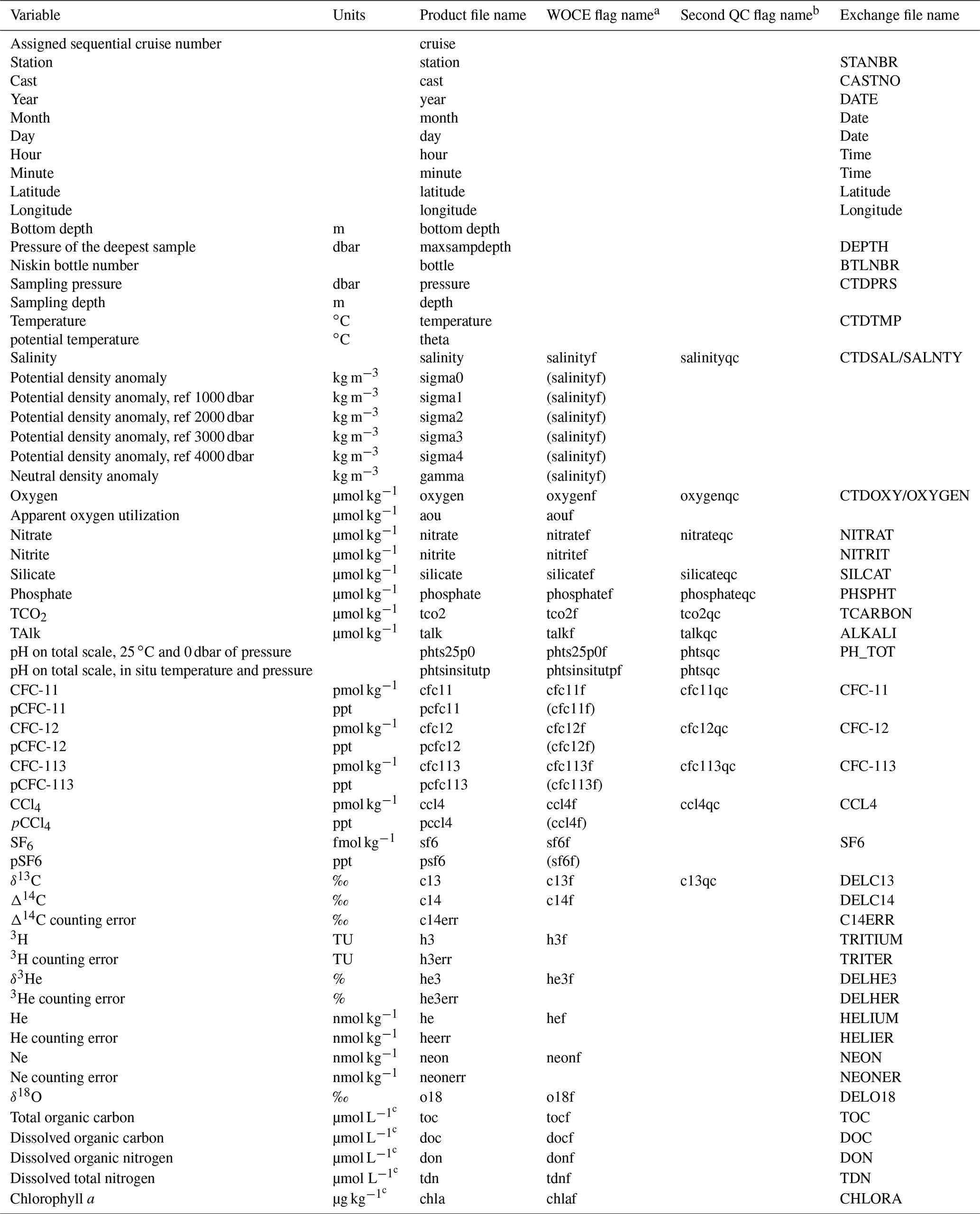
a The only derived variable assigned a separate WOCE flag is AOU as it depends strongly on both temperature and oxygen (and less strongly on salinity). For the other derived variables, the applicable WOCE flag is given in parentheses. b Secondary QC flags indicate whether data have been subjected to full secondary QC (1) or not (0), as described in Sect. 3. c Units have not been checked; some values are in micromoles per kilogram (for TOC, DOC, DON, TDN) or microgram per liter (for Chl a) are probable.
The first version of GLODAP, GLODAPv1.1, was released in 2005 (Key et al., 2004; Sabine et al., 2005). It contains data from 115 cruises with biogeochemical measurements from the global ocean. The vast majority of these are the sections covered during the World Ocean Circulation Experiment and the Joint Global Ocean Flux Study (WOCE/JGOFS) in the 1990s, but data from important “historical” cruises were also included, such as from the Geochemical Ocean Sections Study (GEOSECS), Transient Traces in the Ocean (TTO), and South Atlantic Ventilation Experiment (SAVE). The second version of GLODAP, GLODAPv2, was released in 2016 (Key et al., 2015; Lauvset et al., 2016; Olsen et al., 2016) with data from 724 scientific cruises: those included in GLODAPv1.1, those amassed for the Carbon in the Atlantic Ocean (CARINA) data synthesis (Key et al., 2010); those amassed for the Pacific Ocean Interior Carbon (PACIFICA) synthesis (Suzuki et al., 2013), and data from 168 additional cruises. The additional cruises include many collected within the framework of the “repeat hydrography” program (Talley et al., 2016), instigated in the early 2000s as part of CLIVAR and since 2007 organized as the Global Ocean Ship-based Hydrographic Investigations Program (GO-SHIP). Both GLODAPv1.1 and GLODAPv2 data were released in three formats: (i) as submitted by the data originator but reformatted to WOCE exchange format (Swift and Diggs, 2008) and subjected to primary quality control to flag outliers, (ii) as a merged data product with bias minimization adjustments applied, and (iii) as globally mapped climatological distributions. We refer to the first as the original data, to the second as the data product, and to the third as the mapped product.
The GLODAP products have been widely used. The first version formed the basis for the first data-based estimate of the global ocean inventory of anthropogenic carbon (Sabine et al., 2004), and the descriptive paper on GLODAPv1.1 (Key et al., 2004) has been cited more than 800 times according to Web of Science (Clarivate Analytics). For GLODAPv2, we have registered more than 120 applications. Examples include model evaluation (Beadling et al., 2018; Goris et al., 2018; Tjiputra et al., 2018; Ward et al., 2018), model initialization (Orr et al., 2017), water mass analyses (Jeansson et al., 2017; Peters et al., 2018; Rae and Broecker, 2018), ocean acidification (Fassbender et al., 2017; García-Ibáñez et al., 2016; Perez et al., 2018) calibration of Argo biogeochemical sensor measurements (Bushinsky et al., 2017; Johnson et al., 2017), calibration of multiple linear regression (MLR) and neural-network-based methods for biogeochemical data estimation (Bittig et al., 2018; Carter et al., 2018; Fry et al., 2016; Sauzède et al., 2017), contextualization of paleo-oceanographic data (Glock et al., 2018; Sessford et al., 2018), and calculation of inventory, transport, and variability of ocean carbon (DeVries et al., 2017; Fröb et al., 2016, 2018; Gruber et al., 2019; Panassa et al., 2018; Pardo et al., 2017; Quay et al., 2017). A full list of GLODAPv2 citations is provided at https://www.glodap.info/index.php/glodap-impact/ (last access: 17 September 2019).
Principles and practices for ensuring open access to research data have been established, in particular the Findable, Accessible, Interoperable, Reusable (FAIR) principles (Wilkinson et al., 2016), and are largely adhered to by the oceanographic community. Data are routinely made available on a per cruise basis through national and international data centers. However, the plethora of file formats and different levels of documentation combined with the need to retrieve data on a per cruise basis from different access points limits the realization of the full scientific potential of the data. For biogeochemical data there is the added complexity of different levels of standardization and calibration, and even variable units, such that the comparability between many data sets is poor. Standard operating procedures have been developed for some variables (Dickson et al., 2007; Hood et al., 2010; Hydes et al., 2012) and certified reference materials (CRMs) exist for seawater TCO2 and TAlk measurements (Dickson et al., 2003) and for nutrients in seawater (CRMNS; Aoyama et al., 2012; Ota et al., 2010). Still, biases in data occur. These can arise from poor sampling and general operation practices, calibration procedures, instrument design, and calculations. The use of CRMs does not by itself ensure accurate measurements of seawater CO2 chemistry (Bockmon and Dickson, 2015), and the CRMNS have only become available recently and are not universally used. For salinity and oxygen, lack of – or improper – conductivity–temperature–depth (CTD) sensor calibration is an additional and widespread problem (Olsen et al., 2016). For halogenated transient tracers, uncertainties in the standard gas composition, extracted water volume, and purge efficiency typically provide the largest sources of uncertainty. In addition to bias, occasional outliers occur. In rare cases poor precision can render a set of data unusable. GLODAP deals with these issues by presenting the data in a uniform format, by including any documentation that was either submitted or could be attained, and by subjecting the data to primary and secondary quality control assessments, focusing on precision and consistency, respectively. Adjustments are applied to the data to minimize severe cases of bias.
A total of 12 years separated the release of the two versions of GLODAP. The urgency and complexity of modern climate change issues necessitate more frequent updates. Ocean carbon uptake responds quickly to annual-to-decadal changes in ocean circulation (Fröb et al., 2016; Landschützer et al., 2015), ocean acidification is progressing at unprecedented rates and already causing carbonate mineral undersaturation in some regions (Feely et al., 2008; Qi et al., 2017), oxygen minimum zones are rapidly expanding (Breitburg et al., 2018), and declining nutrient supply to the euphotic zone is potentially changing phytoplankton composition in certain large ocean regions (Rousseaux and Gregg, 2015). In addition, improvements in data management practices and increased computational resources are transforming approaches to, and expectations for, integrated data products. The Surface Ocean CO2 Atlas (SOCAT) is a prominent example in this regard with annual releases and rapid use in global carbon budgets (Bakker et al., 2014, 2016; Le Quéré et al., 2018; Pfeil et al., 2013). GLODAP is also becoming an important source of calibration and validation data for the biogeochemical sensors that are now deployed on autonomous platforms. Altogether, regular and rapid updates are important.
This contribution documents the first such regular update of GLODAP, which adds data from 116 new cruises to the 724 included in GLODAPv2 and corrects errors and omissions in GLODAPv2. It also forms the basis for the documentation of future updates, adopting the Earth System Science Data “living data” format for evolving data sets.
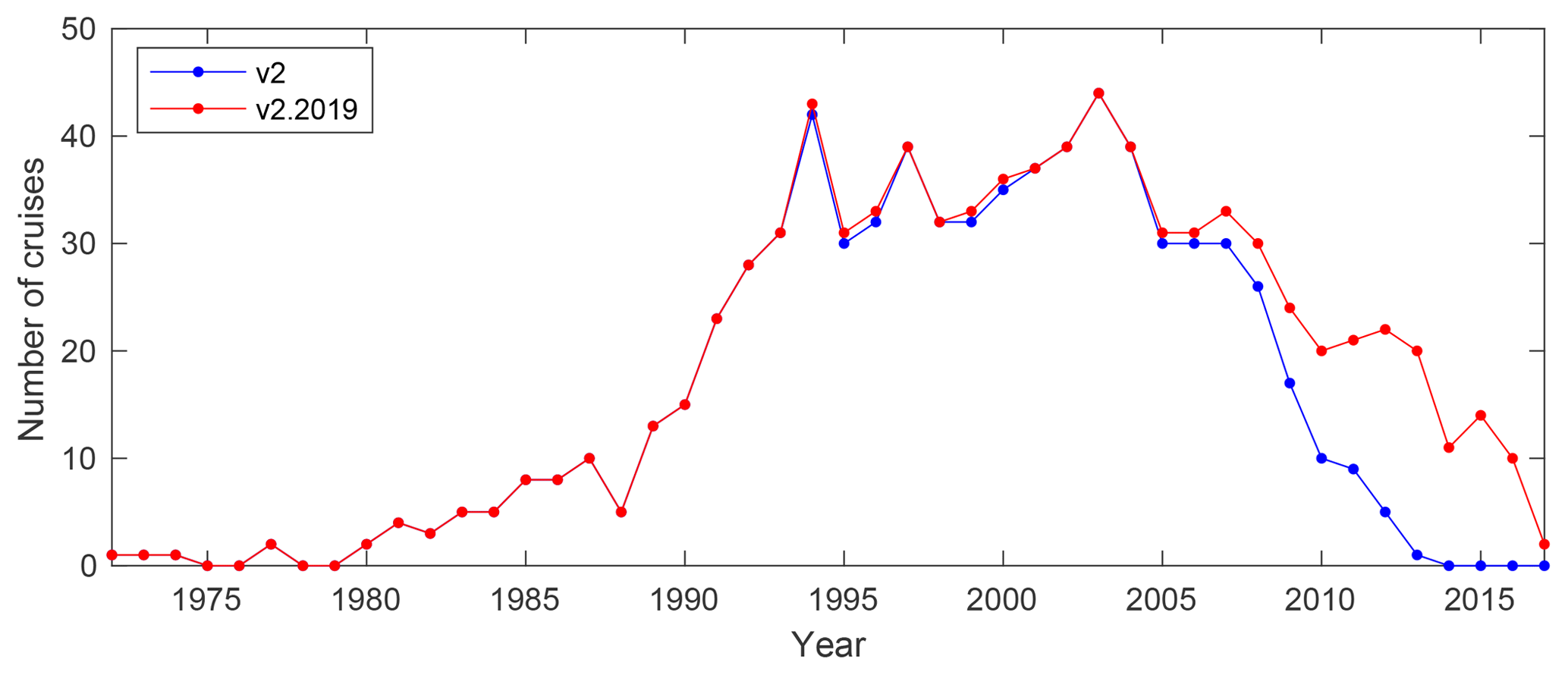
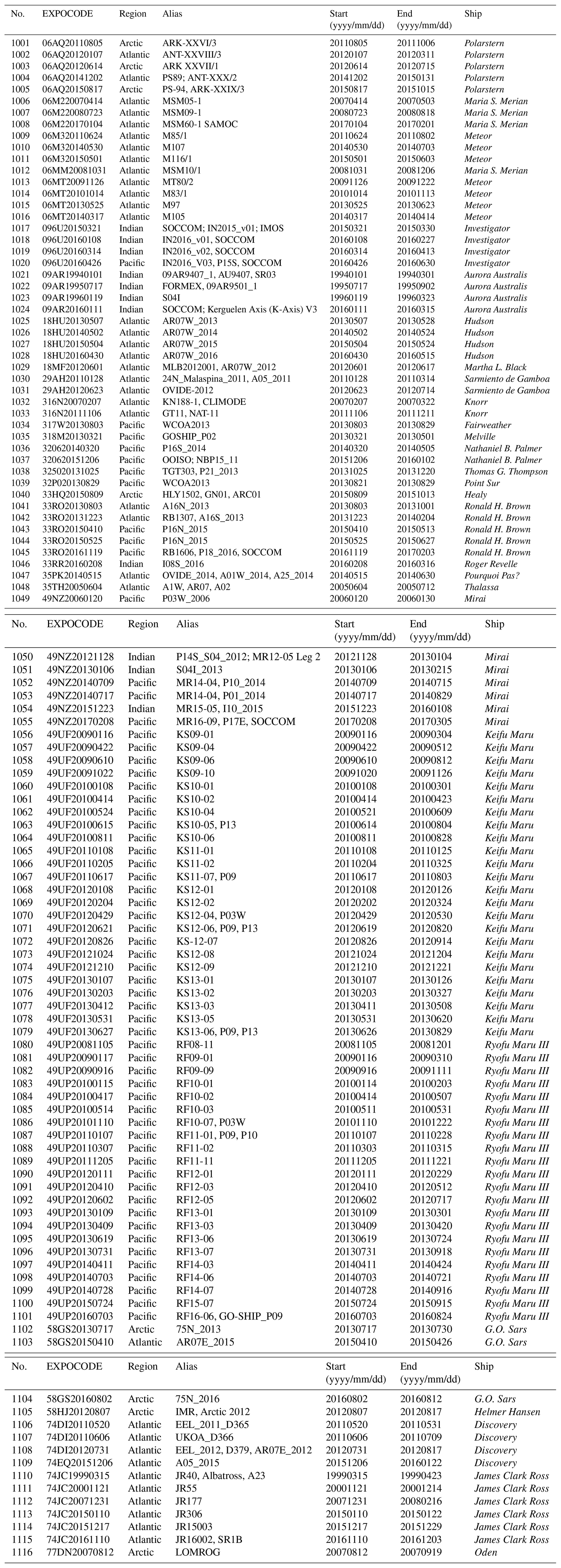
GLODAPv2.2019 (Olsen et al., 2019) contains data from 840 cruises, covering the global ocean from 1972 to 2017. The sampling locations of the 116 cruises added in this update are shown alongside those of GLODAPv2 in Fig. 1, while the coverage in time is shown in Fig. 2. Compared to GLODAPv2, the added data are mostly repeat observations and extend the coverage in time. Information on cruises added to this version is provided in Table A1 in the Appendix.
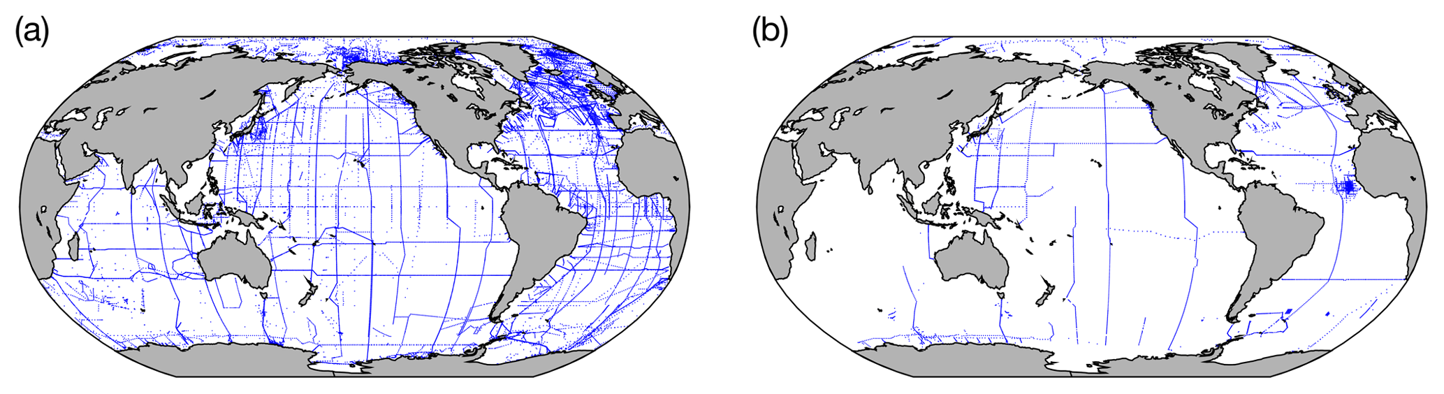
Figure 1Location of stations in (a) GLODAPv2 released in 2016 and for (b) the new data added in this update.
All new cruises were subjected to primary (Sect. 3.1) and secondary (Sect. 3.2) quality control (QC). These procedures remain essentially the same as those for GLODAPv2. However, the secondary QC aimed only to ensure the consistency of the data from the 116 new cruises to GLODAPv2. A consistency analysis of the full GLODAPv2.2019 product (as done with the original GLODAPv2 product) has not been carried out, as it would be too demanding in terms of time and resources to allow for frequent updates, particularly in terms of application of inversion results. The QC of GLODAPv2 produced a sufficiently accurate data set that can serve as a reliable reference (this is in fact already done by some investigators to test their newly collected data; e.g., Panassa et al., 2018). The aim is to conduct a full analysis (i.e., including an inversion) again after the completion of the third GO-SHIP survey, currently scheduled to be completed by 2023. Until that time, intermediate products like this will be released regularly (every 1 or 2 years). A naming convention has been introduced to distinguish intermediate from full product updates. For the latter the version number will change, while for the former the year of release is added.
3.1 Data assembly and primary quality control
The data for the 116 new cruises were retrieved from data centers (typically CCHDO, NCEI, PANGAEA) or submitted directly to us. Each cruise is identified by an EXPOCODE. The EXPOCODE is guaranteed to be unique and constructed by combining the country code and platform code with the date of departure in the format YYYYMMDD. The country and platform codes were taken from the ICES library (https://www.ices.dk/marine-data/vocabularies/Pages/default.aspx, last access: 17 September 2019).
The individual cruise data files were converted to WOCE exchange format: a comma-delimited ASCII format for CTD and bottle data from hydrographic cruises. GLODAP deals only with bottle data, and their exchange format is briefly reviewed here with full details provided in Swift and Diggs (2008). The first line of each exchange file specifies the data type, in the case of GLODAP this is “BOTTLE”, followed by a date and time stamp and identification of the person/group who prepared the file, e.g., “PRINUNIVRMK” is Princeton University, Robert M. Key. Next follows the README section. This provides brief cruise-specific information, such as dates, ship, region, method and quality notes for each variable measured, citation information, and references to any papers that used or presented the data. The README information was typically assembled from the information contained in the metadata submitted by the data originator. In some cases, issues noted during the primary QC and other information such as file update notes are included. The only rule for the README section is that it be concise, informative, and as correct as possible. The README section is followed by data column headers, their units, and then the actual data. The headers and units are standardized and provided in Table 1 for the variables included in GLODAPv2.2019. Exchange file preparation entailed units conversion in some cases, most frequently from milliliters per liter (mL L−1; oxygen) or micromoles per liter (µmol L−1; nutrients) to micromoles per kilogram of seawater (µmol kg−1). The default procedure for nutrients was to use seawater density at reported salinity, an assumed lab temperature of 22 ∘C, and pressure of 1 atm. For oxygen, the factor 44.66 was used for the milliliter to micromole conversion, while for the per liter to per kilogram conversion density based on reported salinity and draw temperatures was preferred, but draw temperature was frequently not reported and potential density was used instead. The potential errors introduced in any of these procedures are insignificant. Missing numbers are indicated by -999, with trailing zeros to comply with the number format for the variable in question, as specified in Swift and Diggs (2008).
Each data column (except temperature and pressure, which are assumed “good” if they exist) has an associated column of data flags. For the exchange files, these flags conform to the WOCE definitions for water sample bottles and are listed in Table 2. If no such WOCE flags were submitted with the data, they were assigned by us. In any case, incoming files were subjected to primary QC to detect questionable or bad data. This was carried out following Sabine et al. (2005) and Tanhua et al. (2010), primarily by inspecting property–property plots. Outliers showing up in two or more different such plots were generally defined as questionable and flagged as such. In some cases, outliers were only detected during the secondary QC; the consequential flag changes have then also been applied in the original cruise data files.
Table 2WOCE flags in GLODAPv2.2019 exchange format original data files and product files.
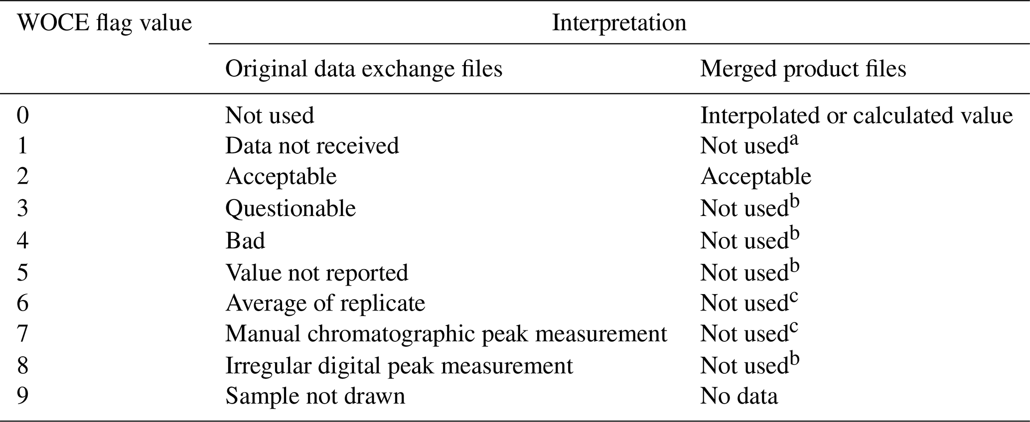
a Flag set to 9 in product files. b Data are not included in the GLODAPv2.2019 product files and their flags set to 9. c Data are included, but flag set to 2.
3.2 Secondary quality control
The aim for the secondary QC was to identify and correct any significant biases in the data from the 116 new cruises relative to GLODAPv2, while retaining any signal due to time changes. To this end, secondary QC in the form of consistency analyses was conducted to identify offsets in the data. All identified offsets were scrutinized by the GLODAP reference group at a meeting in Seattle in September 2018 in order to decide the adjustments to be applied to correct for the offset (if any). To guide this process, a set of initial minimum adjustment limits was used (Table 3). These are set according to the expected measurement precision for each variable, and are the same as those used for GLODAPv2, apart from TAlk and pH. For TAlk the limit was lowered from 6 to 4 µmol kg−1 to better reflect the current level of precision of TAlk measurements (Bockmon and Dickson, 2015). For pH the limit was raised from 0.005 to 0.01, for reasons discussed in Sect. 3.2.4. In addition to the magnitude of the offset, factors such as its precision, persistence towards reference cruises, regional dynamics, and the occurrence of time trends or other variations were considered. Thus, not all offsets larger than the initial minimum limits have been adjusted for. A guiding principle for these considerations was to not apply an adjustment whenever in doubt. In some cases, when data and offsets were very precise and the cruise conducted in a region where variability is expected to be small, adjustments lower than the minimum limits were applied. Any adjustment was applied uniformly to all values for a variable and cruise, i.e., an underlying assumption is that cruises suffer from either no or a single and constant measurement bias. Except for where explicitly noted (Sect. 3.3.1), no adjustments were changed for data previously included in GLODAPv2.

Crossover comparisons, MLRs, and comparison of deep-water averages were used to identify offsets for salinity, oxygen, nutrients, TCO2, and TAlk (Sect. 3.2.2 and 3.2.3). For pH, an additional evaluation of the internal consistency of the seawater CO2 chemistry variables was used whenever possible (Sect. 3.2.4). For the halogenated transient tracers, examination of surface saturation levels and relationship among the tracers were used to assess the data consistency (Sect. 3.4.5). For salinity and oxygen, CTD and bottle values were merged into a “hybrid” variable prior to the consistency analyses (Sect. 3.2.1).
3.2.1 Merging of sensor and bottle data
Salinity and oxygen data can be obtained either by analysis of water samples (bottle data) and/or directly from the CTD sensor pack. These two types are merged and presented as a single variable in the product. The merging was conducted prior to the consistency checks, ensuring their internal calibration in the product. Note that we did not add data from the high-resolution CTD files (as obtained on the downcast) to the bottle data files. The merging procedures were only applied to the bottle data files, which commonly include values recorded by the CTD at the pressures of the upcast when the water samples are collected. Whenever both CTD and bottle data were present in a data file, the merging step considered the deviation between the two and calibrated the CTD values if required and possible. Altogether seven scenarios are possible, where the fourth never occurred during our analyses, but is included to maintain consistency with GLODAPv2. The number of cases encountered for each scenario is summarized in Sect. 4.1.
-
No data are available: no action needed.
-
No bottle values: use CTD values.
-
No CTD values: use bottle values.
-
Too few data of both types for comparison and more than 80 % of the records have bottle values: use bottle values.
-
The CTD values do not deviate significantly from bottle values: replace missing bottle values with CTD values.
-
The CTD values deviate significantly from bottle values: calibrate CTD values using linear fit with respect to bottle data and replace missing bottle values with the so-calibrated CTD values.
-
The CTD values deviate significantly from bottle values, and no good linear fit can be obtained for the cruise: use bottle values and discard CTD values.
3.2.2 Crossover analyses
The crossover analyses were conducted with the MATLAB toolbox prepared by Lauvset and Tanhua (2015) and with the GLODAPv2 data product as reference. In areas where a strong trend in salinity was present, the TAlk and TCO2 data were salinity normalized following Friis et al. (2003), before crossover analysis.
The toolbox implements the “running-cluster” crossover analysis first described by Tanhua et al. (2010). This analysis compares data from two cruises on a station-by-station basis and calculates a weighted mean offset between the two and its weighted standard deviation. The weighting is based on the scatter in the data such that data that have less scatter have a larger influence on the comparison than data with more scatter. Whether the scatter reflects actual variability or data precision is irrelevant in this context as increased scatter regardless decreases the confidence in the comparison. Stations that are compared must be within 2∘ arc distance (∼200 km) of each other, and only deep data are used. This minimizes effects of natural variability. Typically, we used 1500 dbar as the upper depth limit, but in regions where deep mixing occurs (such as the Nordic, Labrador, and Irminger seas) a more conservative limit of 2000 dbar was applied. As an example, the crossover for phosphate as measured on the two cruises 58GS20150410 and 64PE20070830 is shown in Fig. 3. For phosphate the offset is determined as a ratio. This is also the case for the other nutrients, oxygen, and the halogenated transient tracers. For salinity, TCO2, TAlk, and pH, absolute offsets are used, in accordance with the procedures followed for GLODAPv2. The phosphate values from 58GS20150410 are significantly higher, at 1.12±0.016 times those measured at the 64PE20070830 cruise; this is then the weighted mean offset.
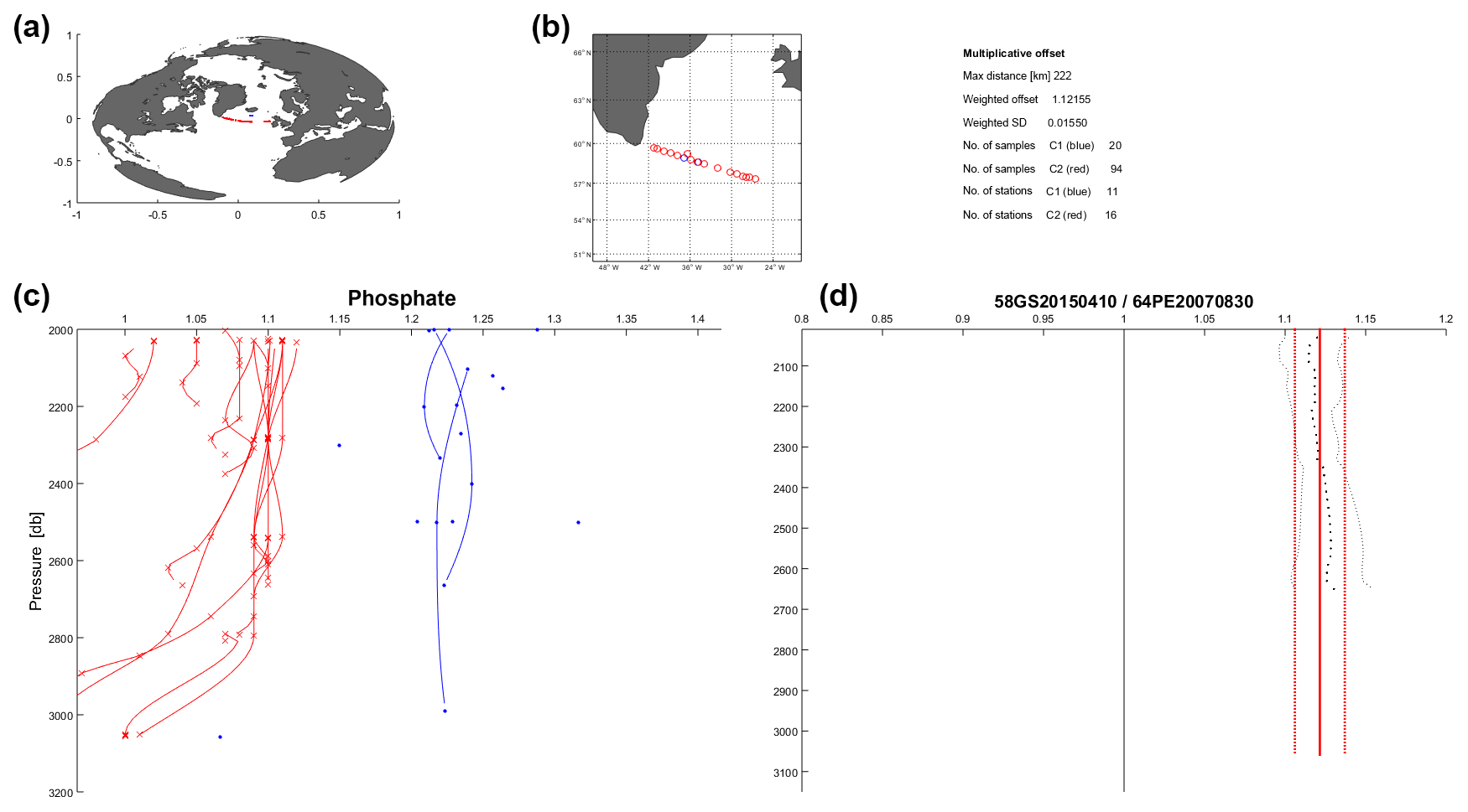
Figure 3Example crossover figure, for phosphate for cruises 58GS20150410 (blue) and 64PE20070830 (red), as it was generated during the crossover analysis. Panels (a) and (b) show the station positions; panel (c) shows the data below the upper depth limit (in this case 2000 dbar as the Irminger Sea is a site of active deep mixing; Fröb et al., 2016) as points and the interpolated profiles as lines. Non-interpolated data either did not meet minimum depth separation requirements (Table 4 in Key et al., 2010) or are the deepest sampling depth. The interpolation do not extrapolate to this. Panel (d) shows the mean difference (as a ratio) profile (black, dots) with its standard deviation, and also the weighted mean offset (straight, red) and weighted standard deviation. Summary statistics are provided in (b).

Figure 4Example summary figure, for phosphate crossovers for 58GS20150410 versus the cruises in GLODAPv2 (with cruise EXPOCODE listed on the x axis sorted according to year the cruise was conducted). The black dots and vertical error bars show the weighted mean offset (as a ratio) and standard deviation for each crossover. The weighted mean of all these offsets is shown in the red line and is 1.13±0.01. The black dashed lines are reference lines for a ±4 % (0.96–1.04) offset. The limit for applying an adjustment for phosphate is half of this, ±2 %.
For each of the 116 new cruises, such a crossover comparison was conducted against all cruises possible in GLODAPv2, i.e., all cruises that had stations closer than 2∘ arc distance to any station for the cruise in question. The summary figure for phosphate at 58GS20150410 is shown in Fig. 4. Clearly, the phosphate data measured at this cruise are high when compared to the data measured at all nearby cruises included in GLODAPv2. An offset of this kind, exceeding the initial minimum adjustment limit (Table 3) and with no obvious time trend, qualifies for an adjustment of the data in the merged data product.
3.2.3 Other consistency analyses
A few new cruises had no or very few valid crossovers with GLODAPv2 data. In that situation two other consistency analyses were carried out for salinity, oxygen, nutrients, TCO2, and TAlk data, namely MLR analyses and deep-water averages, broadly following Jutterström et al. (2010). For the MLRs, the presence of bias in the data for the cruise in question was identified by comparing the MLR generated with the measured value, while for the deep-water averages the approach is trivial. These methods were useful in the data-sparse Arctic and Southern oceans. Both analyses were conducted on samples collected below 1500 or 2000 dbar pressure to minimize the effects of natural variations, and both used available GLODAPv2 data from within 2∘ of the cruise in question to generate the MLR or deep-water average. The lower depth limit was set to the deepest sample for the cruise in question. For the MLRs, all of the abovementioned variables could be included among the independent variables (e.g., for a TAlk MLR, salinity, oxygen, nutrients, and TCO2 were allowed), with the exact selection determined based on the statistical robustness of the fit, as evaluated using the coefficient of determination (r2) and root-mean-square error (RMSE). MLRs that were based on variables that were suspect for the cruise in question were avoided (e.g., if oxygen appeared biased it was not included as an independent variable). The MLRs could be based on 10 to 500 samples, and the robustness of the fit (r2, RMSE) and quantity of fitting data were considered when using the results to guide whether to apply a correction. The same applies for the deep-water averages (i.e., the standard deviation of the mean). MLR and deep-water average results showing offsets above the minimum adjustment limits were carefully scrutinized, along with any crossover results that existed, to determine whether or not to apply an actual adjustment.
3.2.4 pH scale conversion and quality control
A total of 77 of the 116 new cruises included pH data. For about 30 % of these, the pH data were not supplied on the total scale, and at 25 ∘C and 0 dbar pressure, which is the GLODAP standard. These data were converted to total pH scale and temperature and pressure of 25 ∘C and 0 dbar. The conversions were conducted by using CO2SYS (Lewis and Wallace, 1998) for MATLAB (van Heuven et al., 2011) with reported pH and TAlk as inputs, and generating pH output values at total scale at 25 ∘C and 0 dbar of pressure (named phts25p0 in the product). Whenever TAlk data were missing, these values were approximated as 67 times salinity. The proportionality (67) is the mean ratio of TAlk to salinity in the GLODAPv2 data. This is sufficiently accurate for scale–temperature–pressure conversions. Data for phosphate and silicate are also needed and were, whenever missing, determined using CANYON-B (Bittig et al., 2018). The conversion was conducted with the carbonate dissociation constants of Lueker et al. (2000), the bisulfate dissociation constant of Dickson (1990), and the borate-to-salinity ratio of Uppström (1974). These procedures are the same as used for GLODAPv2 (Olsen et al., 2016), except for the CANYON-B estimation of phosphate and silicate.
The secondary quality control of the pH data also followed previous procedures, using a combination of crossovers and internal consistency calculations. The latter were conducted when a cruise had data for TCO2 and TAlk, in addition to pH. Note that internal consistency was only considered for the secondary QC of pH, and not for the secondary QC of TCO2 and TAlk. Hence, the adjustments applied for pH are not only a bias correction but also a seawater CO2 chemistry consistency correction. This is one factor that makes the secondary quality control of pH data problematic, in particular with regard to the application of a uniform correction for an entire cruise or leg based on offsets in deep data. pH dependent offsets between pH determined spectrophotometrically with purified dyes and pH calculated from TCO2 and TAlk have recently been found. For example, at a pH of 7.6 the calculated pH is higher by ∼0.01 than measured pH (Carter et al., 2018). The causes of these discrepancies are not entirely clear, suggestions include deficiencies in dissociation constants used for the seawater CO2 chemistry calculations, errors in the total boron-to-salinity ratio, and unknown protolytes affecting the TAlk (Carter et al., 2018; Fong and Dickson, 2019). Such low pH values exist only in the deep North Pacific Ocean. Here, application of pH corrections based on seawater CO2 consistency considerations could impact the correction. Broadly speaking, the pH data in GLODAP have been obtained using a variety of methods (e.g., potentiometric measurements, and spectrophotometric measurements with purified or impure dyes). The pH values produced by these different approaches have documented pH-dependent offsets from one another (Carter et al., 2013; Liu et al., 2011; Patsavas et al., 2015; Yao et al., 2007) that challenge the viability of the uniform adjustments applied (Carter et al., 2018). While we have continued to apply such uniform offsets for this update, we have chosen the higher initial minimum adjustment limit of 0.01, which is twice that used for GLODAPv2 (0.005), to minimize the possibility of false corrections. The full ramifications and a revised strategy for identifying and minimizing bias in pH data is a topic for future development of the GLODAP data synthesis procedures. The full collection of pH values in GLODAPv2.2019 should only be considered to be consistent between cruises to 0.01 to 0.02 pH units.
3.2.5 Halogenated transient tracers
For the halogenated transient tracers (CFC-11, CFC-12, CFC-113, and CCl4; CFCs for short), inspection of surface saturation levels and evaluation of relationships between the tracers for each cruise were used to identify biases, rather than crossover analyses. Crossover analysis is of limited value for these variables given their transient nature and low deep-water concentrations. As for GLODAPv2, the procedures were the same as those applied for CARINA (Jeansson et al., 2010; Steinfeldt et al., 2010).
3.3 Merged product generation
The merged product file for GLODAPv2.2019 was created by correcting known issues in the GLODAPv2 merged file, and then appending a merged and bias-corrected file containing the 116 new cruises to this error-corrected GLODAPv2 file.
3.3.1 Updates and corrections for GLODAPv2
Several minor omissions and errors have been identified in the GLODAPv2 data product since its release in early 2016. Most of these have been corrected in this release. In addition, some recently available data have been added for a few cruises. The changes are as follows.
-
For 29 cruises spectrophotometric pH data were available but not included in the data product despite having passed secondary quality control. The data from 24 of these cruises are now included, while for the other five cruises the data have been discarded following more in-depth quality control. Whenever possible (Sect. 3.3.2), TAlk or TCO2 was calculated for these cruises as well.
-
The extension “.1” has been removed from the three EXPOCODES 316N19720718.1, 316N19871123.1, and 316N19871123.1.
-
For 33LG20090901 salinity has been included.
-
For 35TH20040604 nutrient data have been replaced with updated data from the PI.
-
For 09AR20071216 TAlk and TCO2 data have been updated.
-
For 33AT20120324 and 33AT20120419 DOC, TAlk, and SF6 data have been updated.
-
For 35UCKERFIXTS TAlk and TCO2 data have been adjusted by −45 and −39 µmol kg−1, respectively.
-
Secondary QC flags for calculated carbon variables are corrected.
-
For 99 records in GLODAPv2 unrealistic differences between sampling pressure and depth were noted. This has been corrected by using the original reported pressure and recalculating depth.
-
Impossible dates (e.g., 31 November) and time stamps (e.g., minute =81) were fixed for a small number of cruises.
-
Recently available/updated data for radioisotope and stable isotopes as well as noble gases were added to eight cruises.
-
For 06AQ19960317 the 3H data have been flagged as bad.
-
For 21 cruises the δ13C values have been adjusted according to the results from Becker et al. (2016). To enable identification of δ13C subjected to secondary QC, a secondary QC flag for δ13C has been included in the GLODAPv2.2019 product file.
-
For 64PE20070830 and 06M220090714 halogenated transient tracer data have been updated.
-
Some outliers detected since the release have been removed (from the merged GLODAPv2.2019 product) and flagged as bad/questionable (in the original cruise data files).
-
Neutral density, γ, was recalculated for the entire product file using the global polynomial of Sérazin (2011), which consists of a set of polynomials for each ocean basin, joined together at their boundaries by weighting functions.
3.3.2 Merging
The new data were merged into a bias-minimized product file following the procedures used for GLODAPv1.1 (Key et al., 2004; Sabine et al., 2005), CARINA (Key et al., 2010), PACIFICA (Suzuki et al., 2013), and GLODAPv2 (Olsen et al., 2016), but with minor changes.
Data from the 116 new cruises were merged and sorted according to EXPOCODE, station, and pressure. Cruise numbers were assigned consecutively, starting from 1001, so they can be distinguished from the GLODAPv2 cruises that ended at 724.
Whenever nitrate plus nitrite were reported instead of nitrate and explicit nitrite concentrations were also given, these were subtracted to get the nitrate values; otherwise, NO3+NO2 was renamed as NO3. As nitrite concentrations are very small in the open ocean, this has no practical implications.
When bottom depths were not given, they were approximated as the deepest sample pressure +10 dbar or extracted from ETOPO1 (Amante and Eakins, 2009), whichever was greater. For GLODAPv2, these values were extracted from the Terrain Base (National Geophysical Data Center/NESDIS/NOAA/U.S. Department of Commerce, 1995). This change has no practical implications, as the variable is only included for drawing approximate bottom topography for sections.
Whenever temperature was missing, all data for that record were removed and their flags set to 9. The same was done when both pressure and depth were missing. For all surface samples collected using buckets or similar, the bottle number was set to zero.
All data with WOCE quality flags 3, 4, 5, or 8 were excluded from the product files (value set to −999/NaN) and their flags set to 9. Hence, in the product files a flag 9 can indicate not measured (as is also the case for the original exchange-formatted data files) or excluded from product; in any case, no data value appears. All flags 6 (good replicate measurement) and 7 (manual chromatographic peak measurement) were set to 2.
Whenever either sampling pressure or depth was missing this was calculated following UNESCO (1981).
For both oxygen and salinity, any reported CTD and bottle values were merged following procedures summarized in Sect. 3.2.1.
Missing salinity, oxygen, nitrate, silicate, and phosphate values were vertically interpolated whenever practical, using a quasi-Hermitian piecewise polynomial. “Whenever practical” means that interpolation was limited to the vertical data separation distances given in Table 4 in Key et al. (2010). Interpolated values have been assigned a WOCE quality flag 0.
Table 4Summary of salinity and oxygen calibration needs and actions; number of occurrences for each of the scenarios identified.

The data for the 12 core variables were corrected for bias using the adjustments determined during the secondary QC. For each of these variables the data product also has separate columns of secondary QC flags, indicating by cruise and variable whether (“1”) or not (“0”) data successfully received secondary QC. A 0 flag here means that data were too shallow or geographically too isolated for consistency analyses. For one of the new cruises, an adjustment that had been recommended for the δ13C data by Becker et al. (2016) was applied.
Values for potential temperature and potential density anomalies (referenced to 0, 1000, 2000, 3000, and 4000 dbar) were calculated following Fofonoff (1977) and Bryden (1973). Neutral density was calculated using Sérazin (2011). Apparent oxygen utilization was determined using the combined fit in Garcia and Gordon (1992).
Partial pressures for CFC-11, CFC-12, CFC-113, CCl4, and SF6 were calculated using the solubilities by Warner and Weiss (1985), Bu and Warner (1995), Bullister and Wisegarver (1998), and Bullister et al. (2002).
Whenever only two seawater CO2 chemistry variables were reported, the third was calculated using CO2SYS (Lewis and Wallace, 1998) for MATLAB (van Heuven et al., 2011), with the constants set as for the pH conversions (Sect. 3.2.4). If this resulted in a mix of measured and calculated values for a certain CO2 system variable for a specific cruise, and if the number of calculated values was equal to or exceeded twice the number of measured values, then all measured values were replaced by calculated values. Calculated values have been assigned WOCE flag 0.
The resulting merged file for the 116 new cruises was appended to the merged product file for GLODAPv2.
All material produced during the secondary QC is available at the online GLODAP Adjustment Table hosted by GEOMAR, Kiel, Germany, at https://glodapv2-2019.geomar.de/ (last access: 17 September 2019), and which can also be accessed through https://www.glodap.info/. This is similar in form and function to the GLODAPv2 Adjustment Table (Olsen et al., 2016) and includes a brief written statement for any adjustments applied.
4.1 Sensor and bottle data merge for salinity and oxygen
Table 4 summarizes the actions taken for the merging of the CTD and bottle data for salinity and oxygen. For most cruises (88 %) both CTD and bottle data were included for salinity in the original cruise data files and for all these cruises the two data types were found to be consistent. For comparison, only 52 % of the GLODAPv2 entries included both, and for a large fraction of these (35 %) the CTD values were uncalibrated (Olsen et al., 2016). For oxygen, 50 % of the cruises included both CTD O2 and bottle values; however, more than a third of these (38 %) had uncalibrated CTD O2 values. For comparison, half of the cruises in GLODAPv2 with both data types (50 %) had uncalibrated CTD O2 (Olsen et al., 2016); this fraction is therefore improving, but it is still too large. Our simple linear calibration gave satisfactory results for eight of these cruises, while for 13 no good fit could be obtained and their CTD O2 data have not been included in the merged product. For data files that only contain bottle values for either or both variables, the tallies are somewhat uncertain, as some CTD values might have been mislabeled by the data originators.
4.2 Adjustment summary
The secondary QC actions for the 12 core variables are summarized in Table 5. Compared to GLODAPv2, the fraction of data that is adjusted is smaller. A percentage of 0 %–10 % of the 116 new cruises are adjusted for each core variable, whereas for the 724 cruises in GLODAPv2, 5 %–30 % were adjusted for each core variable. The number of adjusted cruises is particularly low for salinity (only one of the new cruises was adjusted, i.e., 1 % compared to 5 % for the 724 GLODAPv2 cruises), for the halogenated transient tracers (0 %–3 % adjusted, depending on variable, compared to 6 %–10 % for GLODAPv2), and for TCO2 (two cruises, i.e., 2 % compared to 17 % for GLODAPv2).
Table 5Summary of secondary QC actions per variable for the 116 new cruises.

a The data are included in the data product file as is, with a secondary QC flag of 1. b The adjusted data are included in the data product file with a secondary QC flag of 1. c Data appear of good quality but have not been subjected to full secondary QC. They are included in the data product with a secondary QC flag of 0. d Data are of uncertain quality and suspended until full secondary QC has been carried out; they are excluded from the data product. e Data are of poor quality and excluded from the data product.
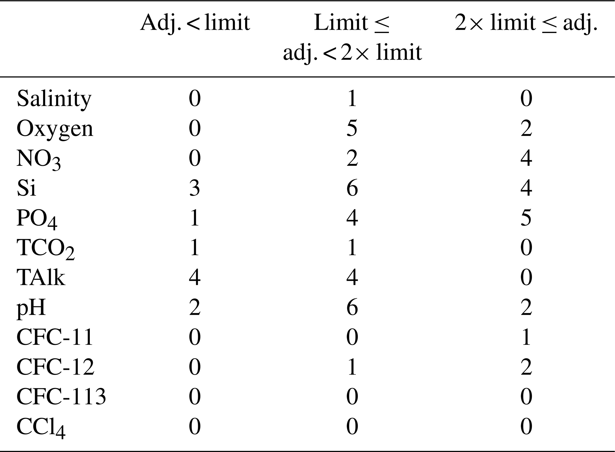
The distributions of the magnitude of adjustments applied are presented in Fig. 5 and Table 6. For salinity, oxygen, and silicate, adjustments between 1 and 2 times the initial minimum adjustment limit are most prevalent. For nitrate, phosphate, CFC-11, and CFC-12, adjustments equal to or larger than 2 times the limit are most prevalent. For the salinity and oxygen this reflects that any biases in the data tend to be between 1 and 2 times the limit, while for CFC-11 and CFC-12 it also likely reflects limitations in our ability to confidently identify small biases. These limitations are related to the strongly transient nature of the CFCs. For TCO2 and TAlk, none of the adjustments are larger than 2 times the adjustment limit, and for both properties half of the adjustments applied are below the limit. For TAlk, this distribution of adjustments supports the lowered minimum adjustment limit of 4 µmol kg−1 (instead of 6 µmol kg−1); these data have sufficient precision to enable the identification of such small adjustments.
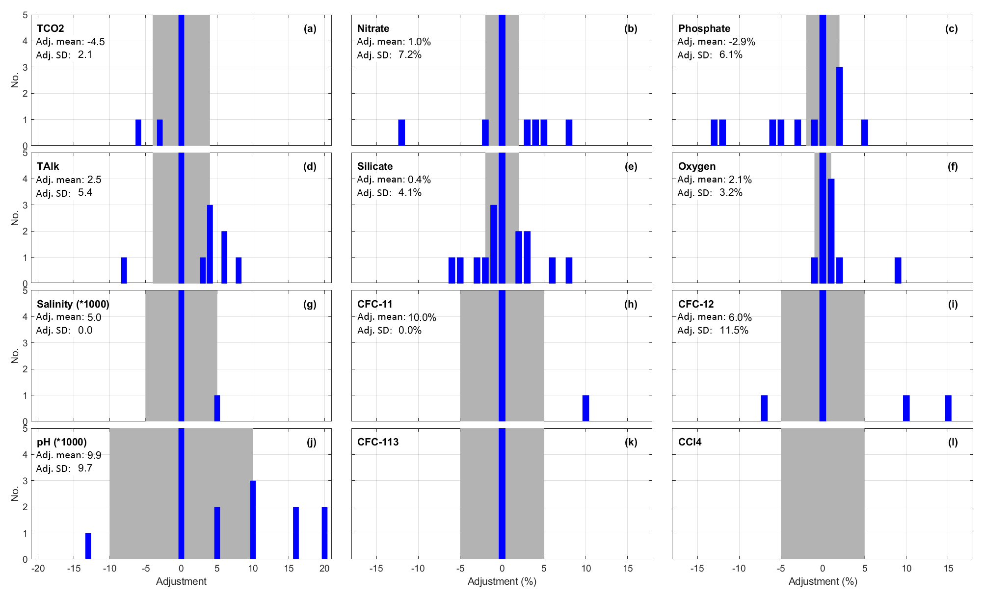
Figure 5Distribution of applied adjustments for each core variable that received secondary QC. Grey areas depict the initial minimum adjustment limits. The figure includes numbers for data subjected to secondary quality control only. Note also that the y-axis scale is set to render the number of adjustments to be visible, so the bar showing zero offset (0 bar) for each variable is cut off (see Table 5 for these numbers).
Table 6Summary of the distribution of applied adjustments per variable, in number of adjustments applied for each variable.
For TAlk, seven out of eight adjustments are positive (i.e., the data are biased low), for pH nine out of 10 adjustments are positive, and for oxygen six out of seven are positive. The adjustments for the other variables were more distributed around zero. For TAlk, prevalence of a negative bias was also observed in the interlaboratory comparison reported by Bockmon and Dickson (2015), who suggested the cause being the use of end point titrations rather than the (preferred) equivalence point titrations. However, six out of seven of the negative bias cruises were Japanese. A tendency for bias in Japanese cruises to be negative was also identified in GLODAPv2 and may be due to the use of internal reference material. We note that the TAlk data from 23 out of 29 Japanese cruises with viable deep crossover checks had no apparent deep offset, so the majority of new TAlk data from Japan were consistent with GLODAPv2 even with the lowered threshold.
The prevalence of positive pH adjustments may relate to the fact that at low pH (as is common in the deeper waters where crossover analyses are done), measurements made with purified dyes tend to be lower than pH determined using electrodes, using impure spectrophotometric dyes with older dye coefficients (Clayton and Byrne, 1993), or calculated from TCO2 and TAlk (Carter et al., 2018). The latter three types of pH data constitute the bulk of the reference data for the consistency checks, so the prevalence of a modern negative bias may be a consequence of limitations in the approaches used for the secondary quality control of the pH data in GLODAP. As mentioned above, refining these should be a priority in the future. Here, we acknowledge the issue and believe that a realistic estimate of the consistency of the pH data in the product is approximately 0.01–0.02.
Crossover comparison is conducted on deep-water samples so atmospheric exchange during sample collection on the new cruises is not a viable explanation for the trend of positive oxygen adjustments. Atmospheric contamination would usually increase deep-water oxygen concentrations since deep oxygen levels are usually low. The data are not collected in any particular region, or associated with any specific laboratory, country, or method. Consequently, no particular explanation can be offered for the prevalence of positive adjustments.
Table 7Improvements resulting from quality control of the 116 new cruises, per basin and for the global data set. The numbers in the table are the weighted mean of the absolute offset of unadjusted and adjusted data versus GLODAPv2. n is the total number of valid crossovers in the global ocean for the variable in question.
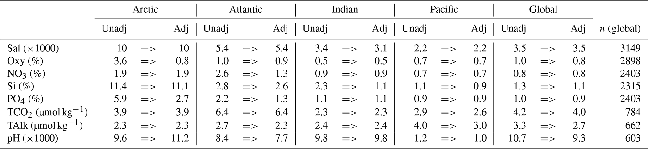
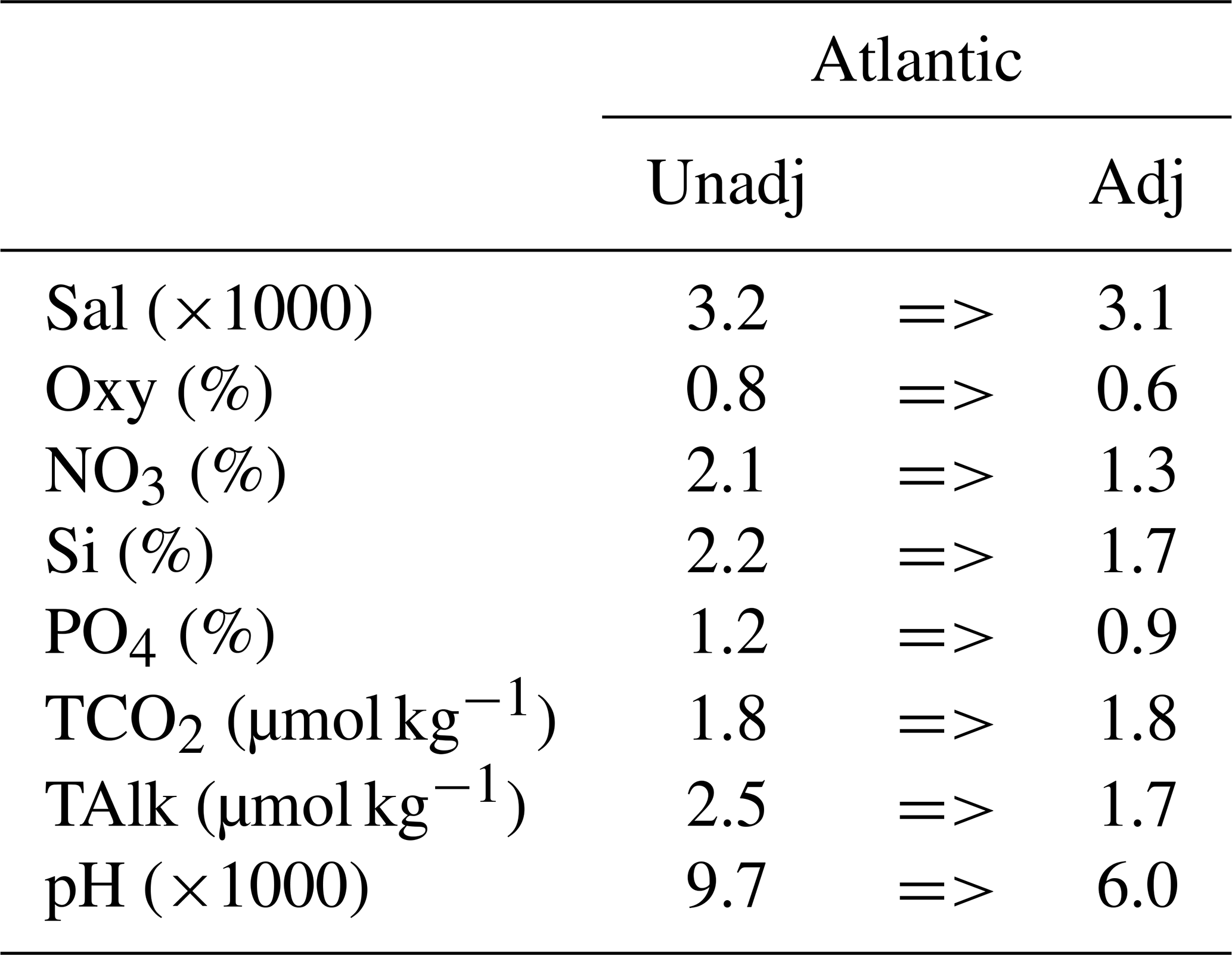
The improvement in data consistency is evaluated by comparing the weighted mean of the absolute offsets for all crossovers before and after the adjustments have been applied. This “consistency improvement” for core variables is presented in Table 7. CFCs were omitted for previously discussed reasons (Sect. 3.2.5). Globally, the improvement is modest, except for TAlk, where the consistency was improved from 3.3 to 2.7 µmol kg−1. Considering the initial data quality, this result was expected. But this does not imply that the data were initially consistent everywhere. Rather, for some regions and variables there are substantial improvements when the adjustments are applied. For example, Arctic Ocean oxygen and phosphate, Atlantic Ocean nitrate and phosphate, Indian Ocean silicate, and Pacific Ocean TAlk data all show considerable improvements.
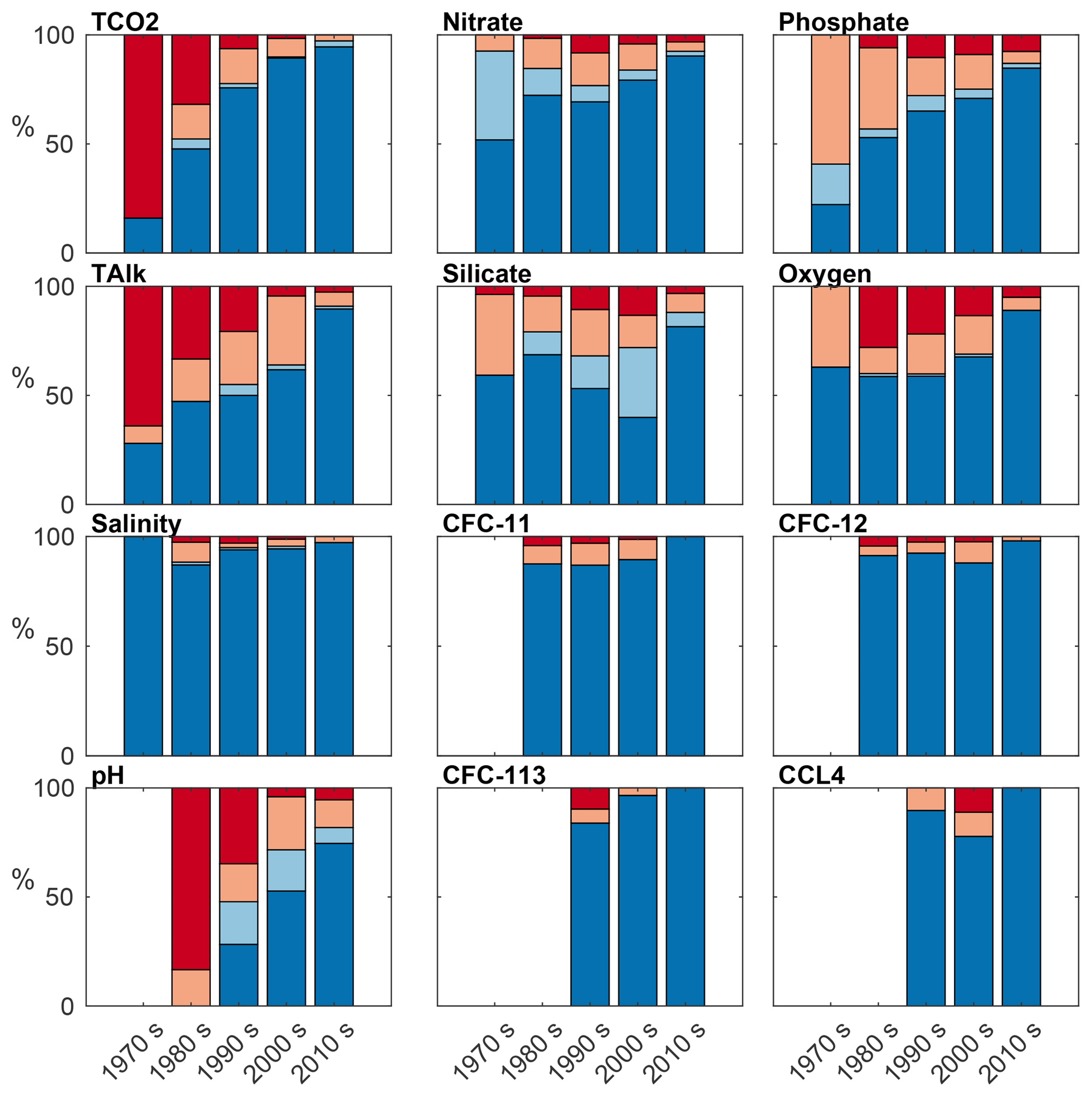
Figure 6Distribution of applied adjustments per decade for the 840 cruises included in GLODAPv2.2019. Dark blue: not adjusted; light blue: absolute adjustment is smaller than initial minimum adjustment limit (Table 3); orange: absolute adjustment is between limit and 2 times the limit, red: absolute adjustment is larger than 2 times the limit.
For the Arctic and Atlantic oceans there are substantial offsets for many variables with respect to GLODAPv2 even after the adjustments have been applied. This relates to actual variability in deep waters of the northern North Atlantic and Arctic regions. For example, the weighted mean of the absolute offset for Arctic Ocean silicate for the adjusted data is 11.1 % and that for salinity is 10 ppm (i.e., a salinity of 0.01). This can be ascribed to two cruises, 58GS20130717 and 58GS20160802, conducted in the Greenland Sea where an increasing presence of Arctic sourced deep waters generates changes in these properties (Blindheim and Rey, 2004; Lauvset et al., 2018; Olafsson and Olsen, 2010; Olsen et al., 2009) that have not been corrected for. The impact of northern variability on the final consistency estimate can be determined for the Atlantic Ocean by excluding all data north of 50∘ N from the analysis. This gives a much better initial and final consistency, on par with that for the Indian and Pacific oceans (Table 8).
Table 8Improvements resulting from the quality control of Atlantic cruises south of 50∘ N.
The various iterations of GLODAP now provide insight into initial data quality covering more than 4 decades. Figure 6 summarizes the applied absolute adjustment magnitude per decade. For several variables improvement is evident over time. Most TCO2 and TAlk data from the 1970s needed an adjustment, but this fraction steadily declines until only a small percentage is adjusted. This is encouraging and demonstrates the value of standardizing sampling and measurement practices (Dickson et al., 2007), the widespread use of CRMs (Dickson et al., 2003), and instrument automation. The pH adjustment frequency also has a downward trend; however, the situation is far from ideal and a topic for future development in GLODAP. For the nutrients and oxygen, only phosphate adjustment frequency decreases from decade to decade. However, we do note that the more recent data, from the 2010s, receive the fewest adjustments. This may reflect recent increased attention that seawater nutrient measurements have received through an operations manual (Hydes et al., 2012), availability of CRMNS (Aoyama et al., 2012; Ota et al., 2010), and SCOR working group no. 147, towards comparability of global oceanic nutrient data (COMPONUT). For silicate, the fraction of cruises receiving adjustments is largest in the 1990s and 2000s. This is related to the 2 % offset between US and Japanese cruises in the Pacific Ocean that was revealed during production of GLODAPv2 and discussed in Olsen et al. (2016). For salinity and the halogenated transient tracers, the number of adjusted cruises is small in every decade.
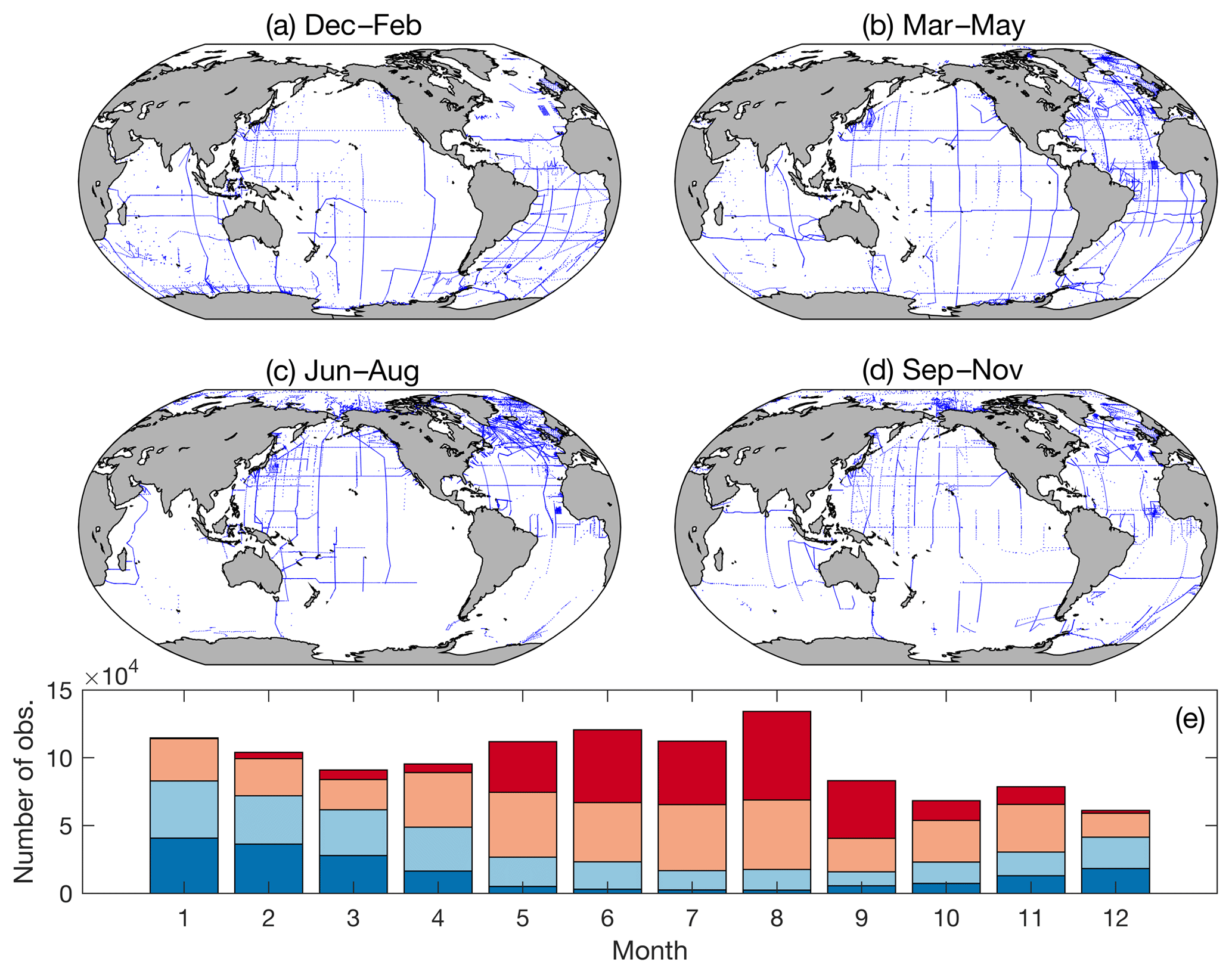
Figure 7Distribution of data in GLODAPv2.2019 in (a) December–February, (b) March–May, (c) June–August, and (d) September–November and (e) number of observations for each month north of 45∘ N (red), north of the Equator to 45∘ N (orange), the Equator to 45∘ S (light blue), and south of 45∘ S (dark blue).
The GLODAPv2.2019 merged and adjusted data product is archived at NOAA NCEI under https://doi.org/10.25921/xnme-wr20 (Olsen et al., 2019). These data and ancillary information are also available via our web pages https://www.glodap.info/ and https://www.nodc.noaa.gov/ocads/oceans/GLODAPv2_2019/ (last access: 19 September 2019). The data are available as comma-separated ascii files (*.csv) and as binary MATLAB files (*.mat). Regional subsets are also available for the Arctic, Atlantic, Pacific, and Indian oceans. There are no data overlaps between regional subsets and each cruise exists in only one basin file even if data from that cruise cross basin boundaries. The station locations in each basin file are shown in Fig. 9. The product file variables are listed in Table 1. A lookup table for matching the EXPOCODE of a cruise with its GLODAP cruise number is provided with the data files. In the MATLAB files this information is also available as a cell array. A “known issues document” accompanies the data files and provides an overview of known errors and omissions in the data product files. It is regularly updated, and users are encouraged to inform us whenever any new issues are identified. It is critical that users consult this document whenever the data products are used.
The original cruise files are available through the GLODAPv2.2019 cruise summary table (CST) hosted by NOAA NCEI: https://www.nodc.noaa.gov/ocads/oceans/GLODAPv2. Each of these files has been assigned a DOI, but these are not listed here. The CST also provides brief information on each cruise and access to metadata, cruise reports, and the Adjustment Table entry for each cruise.
While GLODAPv2.2019 is made available without any restrictions, users of the data should adhere to the fair data use principles.
For investigations that rely on a particular (set of) cruise(s), recognize the contribution of GLODAP data contributors by at least citing the articles where the data are described and, preferably, contacting principal investigators for exploring opportunities for collaboration and co-authorship. To this end, relevant articles and principle investigator names are provided in the CST. This comes with the additional benefit that the principal investigators often possess expert insight into the data and/or particular region under investigation. This can improve scientific quality and promote data sharing.
Cite this paper in any scientific publications that result from usage of the product. Citations provide us with the most efficient means to track the use of this product, which is important for attracting funding to enable the preparation of future updates.
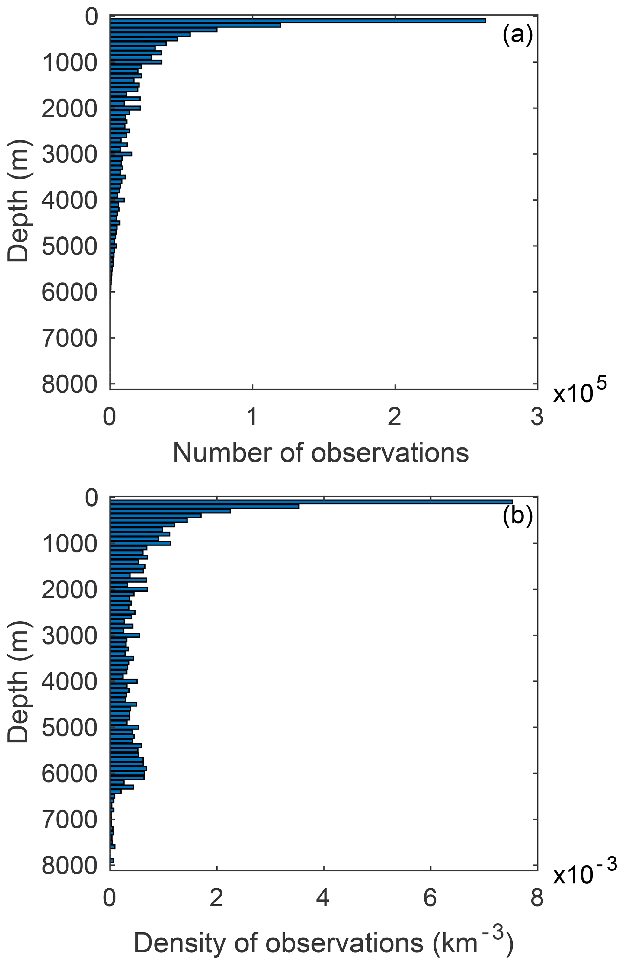
Figure 8Number (a) and density (b) of observations in 100 m depth layers. The latter was calculated by dividing the number of observations in each layer by its global volume calculated from ETOPO2v2 (National Geophysical Data Center, 2006). For example, in the layer between 0 and 100 m there are on average 0.0075 observations per cubic kilometer. One observation is one water sampling point and has data for several variables.
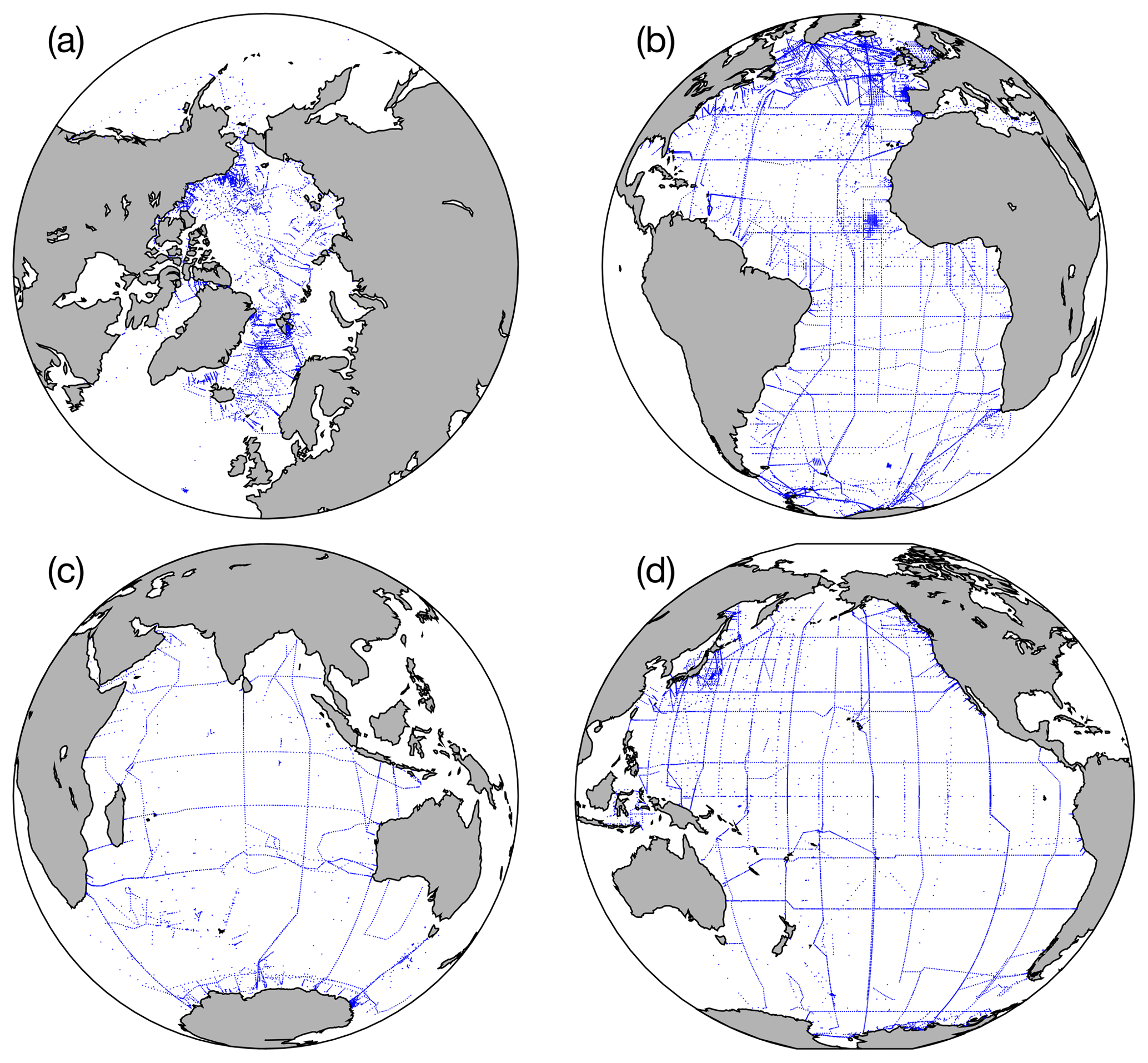
Figure 9Locations of stations included in the (a) Arctic, (b) Atlantic, (c) Indian, and (d) Pacific ocean product files for the whole GLODAPv2.2019 data set.
GLODAPv2.2019 is an update of GLODAPv2. Data from 116 new cruises have been added to supplement the earlier release and extend temporal coverage by 4 years. GLODAP now includes 45 years, 1972–2017, of global interior ocean biogeochemical data from 840 cruises. Figure 7 illustrates the seasonal distribution of the data. There is a bias around summertime in the data in both hemispheres; most data are collected during April through November in the Northern Hemisphere while most data are collected during November through April in the Southern Hemisphere. These tendencies are strongest for the poleward regions and reflect the harsh conditions during winter months, which make fieldwork difficult. Figure 8 illustrates the distribution of data with depth. The upper 100 m is the best sampled part of the global ocean, in terms of both number (Fig. 8a) and density (Fig. 8b) of observations. The number of observations steadily declines with depth. In part, this is caused by the reduction of ocean volume towards greater depths. Below 1000 m the density of observations stabilizes and even increases between 5000 and 6000 m; the latter is a zone where the volume of each depth surface decreases sharply (Weatherall et al., 2015). In the deep trenches, i.e., areas deeper than ∼6000 m, both number and density of observations are fairly low.
Except for salinity and oxygen, the core data were collected exclusively through chemical analyses of individually collected water samples. The data of 12 core variables: salinity, oxygen, nitrate, silicate, phosphate, TCO2, TAlk, pH, CFC-11, CFC-12, CFC-113, and CCl4 were subjected to primary quality control to identify questionable or bad data points (outliers) and secondary quality control to identify systematic measurement biases. The data are provided in two ways: as a set of individual exchange-formatted original cruise data files with assigned WOCE flags, and as globally and regionally merged data product files with adjustments applied to the data according to the outcome of the consistency analyses. Importantly, no adjustments were applied to data in the individual cruise files.
The consistency analyses were conducted by comparing the data from the 116 new cruises to GLODAPv2. Adjustments were only applied when the offsets were believed to reflect biases related to measurement, calibration, and/or data handling practices. The Adjustment Table at https://glodapv2-2019.geomar.de lists all applied adjustments and provides a brief justification for each. The consistency analyses rely on deep ocean data (> 1500 or 2000 dbar depending on region). Data consistency for cruises with exclusively shallow sampling were not examined. Secondary QC flags for the 12 core variables in the product files indicate whether (1) or not (0) the data successfully received secondary QC. If deep data were present, but the consistency analyses were inconclusive, this flag was also set to 0. A secondary QC flag of 0 does not by itself imply that the data are of lower quality than those with a flag of 1. It means these data have not been as thoroughly checked. For δ13C, the QC results by Becker et al. (2016) for the North Atlantic were applied, and a secondary QC flag was therefore added to this variable.
The primary, WOCE, QC flags in the product files are also important, although simplified (e.g., all questionable and bad data were removed). For salinity, oxygen, and the nutrients, any data flagged 0 are interpolated rather than measured. For TCO2, TAlk, and pH, any data flagged 0 are calculated from two measured seawater CO2 variables. Finally, while questionable (WOCE flag =3) and bad (WOCE flag =4) data have been excluded from the product files, some may have gone unnoticed through our analyses. Users are encouraged to report on any data that appear suspicious.
Based on the initial minimum adjustment limits and the improvement of the consistency from the adjustments (Tables 7 and 8), the data subjected to consistency analyses are believed to be consistent to better than 0.005 in salinity, 1 % in oxygen, 2 % in nitrate, 2 % in silicate, 2 % in phosphate, 4 µmol kg−1 in TCO2, and 5 % for the halogenated transient tracers. For TAlk the stated consistency for GLODAPv2 is 6 µmol kg−1 (Olsen et al., 2016). We now believe this is better, 4 µmol kg−1, not only for the 116 new cruises, but also for all data in GLODAPv2 from 2016 as well. This is based on the global average absolute offset for TAlk in the adjusted GLODAPv2 data product of 2.8 µmol kg−1 (Table 5 in Olsen et al., 2016) and the use of the initial minimum adjustment limit of 4 µmol kg−1 for the cruises added with the present version. For pH on the other hand, the consistency among all data is likely not better than 0.01–0.02.
Table A1Cruises included in GLODAPv2.2019 that did not appear in GLODAPv2. Complete information on each cruise, such as variables included and chief scientist and principal investigator names, is provided in the cruise summary table at https://www.nodc.noaa.gov/ocads/oceans/GLODAPv2_2019/cruise_table_v2019.html (last access: 17 September 2019).
AO and TT led the team that produced this update. RMK, AK, MKK, and BP compiled the original data files. NL conducted the secondary QC analyses. CS manages the Adjustment Table e-infrastructure. AK maintains the GLODAPv2 web pages at NCEI/OCADS while SDJ maintains https://www.glodap.info/. All authors contributed to the interpretation of the secondary QC results and decisions on whether to apply actual adjustments. Many conducted ancillary QC analyses. AO wrote the paper with input from all authors.
The authors declare that they have no conflict of interest.
GLODAPv2.2019 would not have been possible without the effort of the many scientists who secured funding, dedicated time to collect, and willingly shared the data that are included. Chief scientists at the various cruises and principal investigators for specific variables are listed in the online cruise summary table.
Meeting and travel support was provided by the IOCCP (via the US National Science Foundation grant OCE-1840868 to the Scientific Committee on Oceanic Research), NOAA PMEL, the AtlantOS project (EU H2020 grant agreement 633211), and the Bjerknes Centre for Climate Research. Henry C. Bittig, Nico Lange, Fiz F. Pérez, Anton Velo, and Siv K. Lauvset were funded by the AtlantOS project. Robert M. Key received partial support from NOAA CICS grant NA14OAR4320106 during the last year of this effort. Contributions from Rik Wanninkhof, Brendan R. Carter, and Richard R. Feely are supported by the Ocean Observing and Monitoring Division, Office of Oceanic and Atmospheric Research of NOAA (data management and synthesis grant N8R3CEA-PDM).
This research has been supported by the Horizon 2020 (AtlantOS (grant no. 633211)), the National Science Foundation (grant no. OCE-1840868), and the National Oceanic and Atmospheric Administration (grant nos. NA14OAR4320106 and N8R3CEAPDM).
This paper was edited by Giuseppe M. R. Manzella and reviewed by Nicolas Gruber and one anonymous referee.
Amante, C. and Eakins, B. W.: ETOPO1 1 Arc-minute global relief model: procedures, data sources and analysis, NOAA Technical Memorandum NESDIS NGDC-24, National Geophysial Data Center, Marine Geology and Geophysics Division, Boulder, CO, USA, 2009.
Aoyama, M., Ota, H., Kimura, M., Kitao, T., Mitsuda, H., Murata, A., and Sato, K.: Current status of homogeneity and stability of the reference materials for nutrients in Seawater, Anal. Sci., 28, 911–916, 2012.
Bakker, D. C. E., Pfeil, B., Smith, K., Hankin, S., Olsen, A., Alin, S. R., Cosca, C., Harasawa, S., Kozyr, A., Nojiri, Y., O'Brien, K. M., Schuster, U., Telszewski, M., Tilbrook, B., Wada, C., Akl, J., Barbero, L., Bates, N. R., Boutin, J., Bozec, Y., Cai, W.-J., Castle, R. D., Chavez, F. P., Chen, L., Chierici, M., Currie, K., de Baar, H. J. W., Evans, W., Feely, R. A., Fransson, A., Gao, Z., Hales, B., Hardman-Mountford, N. J., Hoppema, M., Huang, W.-J., Hunt, C. W., Huss, B., Ichikawa, T., Johannessen, T., Jones, E. M., Jones, S. D., Jutterström, S., Kitidis, V., Körtzinger, A., Landschützer, P., Lauvset, S. K., Lefèvre, N., Manke, A. B., Mathis, J. T., Merlivat, L., Metzl, N., Murata, A., Newberger, T., Omar, A. M., Ono, T., Park, G.-H., Paterson, K., Pierrot, D., Ríos, A. F., Sabine, C. L., Saito, S., Salisbury, J., Sarma, V. V. S. S., Schlitzer, R., Sieger, R., Skjelvan, I., Steinhoff, T., Sullivan, K. F., Sun, H., Sutton, A. J., Suzuki, T., Sweeney, C., Takahashi, T., Tjiputra, J., Tsurushima, N., van Heuven, S. M. A. C., Vandemark, D., Vlahos, P., Wallace, D. W. R., Wanninkhof, R., and Watson, A. J.: An update to the Surface Ocean CO2 Atlas (SOCAT version 2), Earth Syst. Sci. Data, 6, 69–90, https://doi.org/10.5194/essd-6-69-2014, 2014.
Bakker, D. C. E., Pfeil, B., Landa, C. S., Metzl, N., O'Brien, K. M., Olsen, A., Smith, K., Cosca, C., Harasawa, S., Jones, S. D., Nakaoka, S., Nojiri, Y., Schuster, U., Steinhoff, T., Sweeney, C., Takahashi, T., Tilbrook, B., Wada, C., Wanninkhof, R., Alin, S. R., Balestrini, C. F., Barbero, L., Bates, N. R., Bianchi, A. A., Bonou, F., Boutin, J., Bozec, Y., Burger, E. F., Cai, W.-J., Castle, R. D., Chen, L., Chierici, M., Currie, K., Evans, W., Featherstone, C., Feely, R. A., Fransson, A., Goyet, C., Greenwood, N., Gregor, L., Hankin, S., Hardman-Mountford, N. J., Harlay, J., Hauck, J., Hoppema, M., Humphreys, M. P., Hunt, C. W., Huss, B., Ibánhez, J. S. P., Johannessen, T., Keeling, R., Kitidis, V., Körtzinger, A., Kozyr, A., Krasakopoulou, E., Kuwata, A., Landschützer, P., Lauvset, S. K., Lefèvre, N., Lo Monaco, C., Manke, A., Mathis, J. T., Merlivat, L., Millero, F. J., Monteiro, P. M. S., Munro, D. R., Murata, A., Newberger, T., Omar, A. M., Ono, T., Paterson, K., Pearce, D., Pierrot, D., Robbins, L. L., Saito, S., Salisbury, J., Schlitzer, R., Schneider, B., Schweitzer, R., Sieger, R., Skjelvan, I., Sullivan, K. F., Sutherland, S. C., Sutton, A. J., Tadokoro, K., Telszewski, M., Tuma, M., van Heuven, S. M. A. C., Vandemark, D., Ward, B., Watson, A. J., and Xu, S.: A multi-decade record of high-quality fCO2 data in version 3 of the Surface Ocean CO2 Atlas (SOCAT), Earth Syst. Sci. Data, 8, 383–413, https://doi.org/10.5194/essd-8-383-2016, 2016.
Beadling, R. L., Russell, J. L., Stouffer, R. J., and Goodman, P. J.: Evaluation of subtropical North Atlantic Ocean circulation in CMIP5 models against the observational Array at 26.5 degrees N and its changes under continued warming, J. Climate, 31, 9697–9718, 2018.
Becker, M., Andersen, N., Erlenkeuser, H., Humphreys, M. P., Tanhua, T., and Körtzinger, A.: An internally consistent dataset of δ13C-DIC in the North Atlantic Ocean – NAC13v1, Earth Syst. Sci. Data, 8, 559–570, https://doi.org/10.5194/essd-8-559-2016, 2016.
Bittig, H. C., Steinhoff, T., Claustre, H., Fiedler, B., Williams, N. L., Sauzède, R., Körtzinger, A., and Gattuso, J.-P.: An alternative to static climatologies: Robust estimation of open ocean CO2 variables and nutrient concentrations from T, S, and O2 data using Bayesian Neural Networks, Frontiers in Marine Science, 5, 328, https://doi.org/10.3389/fmars.2018.00328, 2018.
Blindheim, J. and Rey, F.: Water-mass formation and distribution in the Nordic Seas during the 1990s, ICES J. Mar. Sci., 61, 846–863, 2004.
Bockmon, E. E. and Dickson, A. G.: An inter-laboratory comparison assessing the quality of seawater carbon dioxide measurements, Mar. Chem., 171, 36–43, 2015.
Breitburg, D., Levin, L. A., Oschlies, A., Grégoire, M., Chavez, F. P., Conley, D. J., Garçon, V., Gilbert, D., Gutiérrez, D., Isensee, K., Jacinto, G. S., Limburg, K. E., Montes, I., Naqvi, S. W. A., Pitcher, G. C., Rabalais, N. N., Roman, M. R., Rose, K. A., Seibel, B. A., Telszewski, M., Yasuhara, M., and Zhang, J.: Declining oxygen in the global ocean and coastal waters, Science, 359, eaam7240, https://doi.org/10.1126/science.aam7240, 2018.
Bryden, H. L.: New polynomials for thermal-expansion, adiabatic temperature gradient and potential temperature of sea-water, Deep-Sea Res., 20, 401–408, 1973.
Bu, X. and Warner, M. J.: Solubility of chlorofluorocarbon-113 in water and seawater, Deep-Sea Res. Pt. I, 42, 1151–1161, 1995.
Bullister, J. L. and Wisegarver, D. P.: The solubility of carbon tetrachloride in water and seawater, Deep-Sea Res. Pt. I, 45, 1285–1302, 1998.
Bullister, J. L., Wisegarver, D. P., and Menzia, F. A.: The solubility of sulfur hexafluoride in water and seawater, Deep-Sea Res. Pt. I, 49, 175–187, 2002.
Bushinsky, S. M., Gray, A. R., Johnson, K. S., and Sarmiento, J. L.: Oxygen in the Southern Ocean from Argo floats: Determination of processes driving air-sea fluxes, J. Geophys. Res.-Oceans, 122, 8661–8682, 2017.
Carter, B. R., Radich, J. A., Doyle, H. L., and Dickson, A. G.: An automated system for spectrophotometric seawater pH measurements, Limnol. Oceanogr.-Meth., 11, 16–27, 2013.
Carter, B. R., Feely, R. A., Williams, N. L., Dickson, A. G., Fong, M. B., and Takeshita, Y.: Updated methods for global locally interpolated estimation of alkalinity, pH, and nitrate, Limnol. Oceanogr.-Meth., 16, 119–131, 2018.
Cheng, L. J., Trenberth, K. E., Fasullo, J., Boyer, T., Abraham, J., and Zhu, J.: Improved estimates of ocean heat content from 1960 to 2015, Sci. Adv., 3, e1601545, https://doi.org/10.1126/sciadv.1601545, 2017.
Clayton, T. D. and Byrne, R. H.: Spectrophotometric seawater pH measurements – Total hydrogen-ion concentration scale calibration of m-cresol purple and at-sea results, Deep-Sea Res. Pt. I, 40, 2115–2129, 1993.
DeVries, T., Holzer, M., and Primeau, F.: Recent increase in oceanic carbon uptake driven by weaker upper-ocean overturning, Nature, 542, 215–218, 2017.
Dickson, A. G.: Standard potential of the reaction: AgCl(s) H2(g) = Ag(s) + HCl(aq) and the standard acidity constant of the ion in synthetic sea water from 273.15 to 318.15 K, J. Chem. Thermodyn., 22, 113–127, 1990.
Dickson, A. G., Afghan, J. D., and Anderson, G. C.: Reference materials for oceanic CO2 analysis: a method for the certification of total alkalinity, Mar. Chem., 80, 185–197, 2003.
Dickson, A. G., Sabine, C. L., and Christian, J. R.: Guide to Best Practices for Ocean CO2 measurements, PICES Special Publication 3, 191 pp., 2007.
Fassbender, A. J., Sabine, C. L., and Palevsky, H. I.: Nonuniform ocean acidification and attenuation of the ocean carbon sink, Geophys. Res. Lett., 44, 8404–8413, 2017.
Feely, R. A., Sabine, C. L., Hernandez-Ayon, J. M., Ianson, D., and Hales, B.: Evidence for upwelling of corrosive “acidified” water onto the continental shelf, Science, 320, 1490–1492, 2008.
Fofonoff, N. P.: Computation of potential temperature of seawater for an arbitrary reference pressure, Deep-Sea Res., 24, 489–491, 1977.
Fong, M. B. and Dickson, A. G.: Insights from GO-SHIP hydrography data into the thermodynamic consistency of CO2 system measurements in seawater, Mar. Chem., 211, 52–63, https://doi.org/10.1016/j.marchem.2019.03.006, 2019.
Friis, K., Körtzinger, A., and Wallace, D. W. R.: The salinity normalization of marine inorganic carbon chemistry data, Geophys. Res. Lett., 30, 1085, https://doi.org/10.1029/2002gl015898, 2003.
Fröb, F., Olsen, A., Vage, K., Moore, G. W. K., Yashayaev, I., Jeansson, E., and Rajasakaren, B.: Irminger Sea deep convection injects oxygen and anthropogenic carbon to the ocean interior, Nat. Commun., 7, 13244, https://doi.org/10.1038/ncomms13244, 2016.
Fröb, F., Olsen, A., Pérez, F. F., García-Ibáñez, M. I., Jeansson, E., Omar, A., and Lauvset, S. K.: Inorganic carbon and water masses in the Irminger Sea since 1991, Biogeosciences, 15, 51–72, https://doi.org/10.5194/bg-15-51-2018, 2018.
Fry, C. H., Tyrrell, T., and Achterberg, E. P.: Analysis of longitudinal variations in North Pacific alkalinity to improve predictive algorithms, Global Biogeochem. Cy., 30, 1493–1508, 2016.
Garcia, H. E. and Gordon, L. I.: Oxygen solubility in seawater – Better fitting equations, Limnol. Oceanogr., 37, 1307–1312, 1992.
García-Ibáñez, M. I., Zunino, P., Fröb, F., Carracedo, L. I., Ríos, A. F., Mercier, H., Olsen, A., and Pérez, F. F.: Ocean acidification in the subpolar North Atlantic: rates and mechanisms controlling pH changes, Biogeosciences, 13, 3701–3715, https://doi.org/10.5194/bg-13-3701-2016, 2016.
Glock, N., Erdem, Z., Wallmann, K., Somes, C. J., Liebetrau, V., Schonfeld, J., Gorb, S., and Eisenhauer, A.: Coupling of oceanic carbon and nitrogen facilitates spatially resolved quantitative reconstruction of nitrate inventories, Nat. Commun., 9, 1217, https://doi.org/10.1038/s41467-018-03647-5, 2018.
Goris, N., Tjiputra, J. F., Olsen, A., Schwinger, J., Lauvset, S. K., and Jeansson, E.: Constraining projection-based estimates of the future North Atlantic carbon uptake, J. Climate, 31, 3959–3978, 2018.
Gruber, N., Clement, D., Carter, B. R., Feely, R. A., van Heuven, S., Hoppema, M., Ishii, M., Key, R. M., Kozyr, A., Lauvset, S. K., Lo Monaco, C., Mathis, J. T., Murata, A., Olsen, A., Perez, F. F., Sabine, C. L., Tanhua, T., and Wanninkhof, R.: The oceanic sink for anthropogenic CO2 from 1994 to 2007, Science, 363, 1193–1199, 2019.
Hood, E. M., Sabine, C. L., and Sloyan, B. M. (Eds.): The GO-SHIP Repeat Hydrography Manual: A Collection of Expert Reports and Guidelines, IOCCP Report Number 14, ICPO Publication Series Number 134, available at: http://www.go-ship.org/HydroMan.html (last access: 17 September 2019), 2010.
Hydes, D. J., Aoyama, A., Aminot, A., Bakker, K., Becker, S., Coverly, S., Daniel, A., Dickson, A. G., Grosso, O., Kerouel, R., van Ooijen, J., Sato, K., Tanhua, T., Woodward, E. M. S., and Zhang, J.-Z.: Determination of dissolved nutrients in seawater with high precision and intercomparability using gas-segmented continuous flow analysers, in: The GO SHIP Repeat Hydrography Manual: A Collection of Expert Reports and Guidelines, edited by: Hood, E. M., Sabine, C., and Sloyan, B. M., IOCCP Report Number 14, ICPO Publication Series Number 134, 2012.
Jeansson, E., Olsen, A., and Jutterström, S.: Arctic Intermediate Water in the Nordic Seas, 1991–2009, Deep-Sea Res. Pt. I, 128, 82–97, 2017.
Jeansson, E., Olsson, K. A., Tanhua, T., and Bullister, J. L.: Nordic Seas and Arctic Ocean CFC data in CARINA, Earth Syst. Sci. Data, 2, 79–97, https://doi.org/10.5194/essd-2-79-2010, 2010.
Jenkins, W. J., Doney, S. C., Fendrock, M., Fine, R., Gamo, T., Jean-Baptiste, P., Key, R., Klein, B., Lupton, J. E., Newton, R., Rhein, M., Roether, W., Sano, Y., Schlitzer, R., Schlosser, P., and Swift, J.: A comprehensive global oceanic dataset of helium isotope and tritium measurements, Earth Syst. Sci. Data, 11, 441–454, https://doi.org/10.5194/essd-11-441-2019, 2019.
Johnson, K. S., Plant, J. N., Coletti, L. J., Jannasch, H. W., Sakamoto, C. M., Riser, S. C., Swift, D. D., Williams, N. L., Boss, E., Haentjens, N., Talley, L. D., and Sarmiento, J. L.: Biogeochemical sensor performance in the SOCCOM profiling float array, J. Geophys. Res.-Oceans, 122, 6416–6436, 2017.
Jutterström, S., Anderson, L. G., Bates, N. R., Bellerby, R., Johannessen, T., Jones, E. P., Key, R. M., Lin, X., Olsen, A., and Omar, A. M.: Arctic Ocean data in CARINA, Earth Syst. Sci. Data, 2, 71–78, https://doi.org/10.5194/essd-2-71-2010, 2010.
Key, R. M., Kozyr, A., Sabine, C. L., Lee, K., Wanninkhof, R., Bullister, J. L., Feely, R. A., Millero, F. J., Mordy, C., and Peng, T. H.: A global ocean carbon climatology: Results from Global Data Analysis Project (GLODAP), Global Biogeochem. Cy., 18, GB4031, https://doi.org/10.1029/2004GB002247, 2004.
Key, R. M., Tanhua, T., Olsen, A., Hoppema, M., Jutterström, S., Schirnick, C., van Heuven, S., Kozyr, A., Lin, X., Velo, A., Wallace, D. W. R., and Mintrop, L.: The CARINA data synthesis project: introduction and overview, Earth Syst. Sci. Data, 2, 105–121, https://doi.org/10.5194/essd-2-105-2010, 2010.
Key, R. M., Olsen, A., van Heuven, S., Lauvset, S. K., Velo, A., Lin, X., Schirnick, C., Kozyr, A., Tanhua, T., Hoppema, M., Jutterstrom, S., Steinfeldt, R., Jeansson, E., Ishii, M., Perez, F. F., and Suzuki, T.: Global Ocean Data Analysis Project, Version 2 (GLODAPv2), ORNL/CDIAC-162, ND-P093., Carbon Dioxide Information Analysis Center, Oak Ridge National Laboratory, US Department of Energy, Oak Ridge, Tennessee, 2015.
Landschützer, P., Gruber, N., Haumann, A., Rodenbeck, C., Bakker, D. C. E., van Heuven, S., Hoppema, M., Metzl, N., Sweeney, C., Takahashi, T., Tilbrook, B., and Wanninkhof, R.: The reinvigoration of the Southern Ocean carbon sink, Science, 349, 1221–1224, 2015.
Lauvset, S. K. and Tanhua, T.: A toolbox for secondary quality control on ocean chemistry and hydrographic data, Limnol. Oceanogr.-Meth., 13, 601–608, 2015.
Lauvset, S. K., Key, R. M., Olsen, A., van Heuven, S., Velo, A., Lin, X., Schirnick, C., Kozyr, A., Tanhua, T., Hoppema, M., Jutterström, S., Steinfeldt, R., Jeansson, E., Ishii, M., Perez, F. F., Suzuki, T., and Watelet, S.: A new global interior ocean mapped climatology: the GLODAP version 2, Earth Syst. Sci. Data, 8, 325–340, https://doi.org/10.5194/essd-8-325-2016, 2016.
Lauvset, S. K., Brakstad, A., Vage, K., Olsen, A., Jeansson, E., and Mork, K. A.: Continued warming, salinification and oxygenation of the Greenland Sea gyre, Tellus A, 70, 1–9, 2018.
Le Quéré, C., Andrew, R. M., Friedlingstein, P., Sitch, S., Hauck, J., Pongratz, J., Pickers, P. A., Korsbakken, J. I., Peters, G. P., Canadell, J. G., Arneth, A., Arora, V. K., Barbero, L., Bastos, A., Bopp, L., Chevallier, F., Chini, L. P., Ciais, P., Doney, S. C., Gkritzalis, T., Goll, D. S., Harris, I., Haverd, V., Hoffman, F. M., Hoppema, M., Houghton, R. A., Hurtt, G., Ilyina, T., Jain, A. K., Johannessen, T., Jones, C. D., Kato, E., Keeling, R. F., Goldewijk, K. K., Landschützer, P., Lefèvre, N., Lienert, S., Liu, Z., Lombardozzi, D., Metzl, N., Munro, D. R., Nabel, J. E. M. S., Nakaoka, S., Neill, C., Olsen, A., Ono, T., Patra, P., Peregon, A., Peters, W., Peylin, P., Pfeil, B., Pierrot, D., Poulter, B., Rehder, G., Resplandy, L., Robertson, E., Rocher, M., Rödenbeck, C., Schuster, U., Schwinger, J., Séférian, R., Skjelvan, I., Steinhoff, T., Sutton, A., Tans, P. P., Tian, H., Tilbrook, B., Tubiello, F. N., van der Laan-Luijkx, I. T., van der Werf, G. R., Viovy, N., Walker, A. P., Wiltshire, A. J., Wright, R., Zaehle, S., and Zheng, B.: Global Carbon Budget 2018, Earth Syst. Sci. Data, 10, 2141–2194, https://doi.org/10.5194/essd-10-2141-2018, 2018.
Lewis, E. and Wallace, D. W. R.: Program developed for CO2 system calculations, ORNL/CDIAC-105, Carbon Dioxide Information Analysis Center, Oak Ridge National Laboratory, Oak Ridge, TN, USA, 1998.
Liu, X. W., Patsavas, M. C., and Byrne, R. H.: Purification and characterization of meta-cresol purple for spectrophotometric seawater pH measurements, Environ. Sci. Technol., 45, 4862–4868, 2011.
Lueker, T. J., Dickson, A. G., and Keeling, C. D.: Ocean pCO2 calculated from dissolved inorganic carbon, alkalinity, and equations for K-1 and K-2: validation based on laboratory measurements of CO2 in gas and seawater at equilibrium, Mar. Chem., 70, 105–119, 2000.
National Geophysical Data Center: 2-minute Gridded Global Relief Data (ETOPO2) v2. National Geophysical Data Center, NOAA, https://doi.org/10.7289/V5J1012Q, 2006.
National Geophysical Data Center/NESDIS/NOAA/U.S. Department of Commerce: TerrainBase, Global 5 Arc-minute Ocean Depth and Land Elevation from the US National Geophysical Data Center (NGDC). Research Data Archive at the National Center for Atmospheric Research, Computational and Information Systems Laboratory, https://doi.org/10.5065/E08M-4482, 1995.
Olafsson, J. and Olsen, A.: Nordic Seas nutrients data in CARINA, Earth Syst. Sci. Data, 2, 205–213, https://doi.org/10.5194/essd-2-205-2010, 2010.
Olsen, A., Key, R. M., Jeansson, E., Falck, E., Olafsson, J., van Heuven, S., Skjelvan, I., Omar, A. M., Olsson, K. A., Anderson, L. G., Jutterström, S., Rey, F., Johannessen, T., Bellerby, R. G. J., Blindheim, J., Bullister, J. L., Pfeil, B., Lin, X., Kozyr, A., Schirnick, C., Tanhua, T., and Wallace, D. W. R.: Overview of the Nordic Seas CARINA data and salinity measurements, Earth Syst. Sci. Data, 1, 25–34, https://doi.org/10.5194/essd-1-25-2009, 2009.
Olsen, A., Key, R. M., van Heuven, S., Lauvset, S. K., Velo, A., Lin, X., Schirnick, C., Kozyr, A., Tanhua, T., Hoppema, M., Jutterström, S., Steinfeldt, R., Jeansson, E., Ishii, M., Pérez, F. F., and Suzuki, T.: The Global Ocean Data Analysis Project version 2 (GLODAPv2) – an internally consistent data product for the world ocean, Earth Syst. Sci. Data, 8, 297–323, https://doi.org/10.5194/essd-8-297-2016, 2016.
Olsen, A., Lange, N., Key, R. M., Tanhua, T., Àlvarez, M., Becker, S., Bittig, H. C., Carter, B. R., Cotrim da Cunha, L., Feely, R. A., van Heuven, S., Hoppema, M., Ishii, M., Jeansson, E., Jones, S. D., Jutterström, S., Karlsen, M. K., Kozyr, A., Lauvset, S. K., Lo Monaco, C., Murata, A., Pérez, F. F., Pfeil, B., Schirnick, C., Steinfeldt, R., Suzuki, T., Telszewski, M., Tilbrook, B., Velo, A., and Wanninkhof, R.: Global Ocean Data Analysis Project, version 2.2019 (GLODAPv2.2019), NOAA National Centers for Environmental Information, https://doi.org/10.25921/xnme-wr20, 2019.
Orr, J. C., Najjar, R. G., Aumont, O., Bopp, L., Bullister, J. L., Danabasoglu, G., Doney, S. C., Dunne, J. P., Dutay, J.-C., Graven, H., Griffies, S. M., John, J. G., Joos, F., Levin, I., Lindsay, K., Matear, R. J., McKinley, G. A., Mouchet, A., Oschlies, A., Romanou, A., Schlitzer, R., Tagliabue, A., Tanhua, T., and Yool, A.: Biogeochemical protocols and diagnostics for the CMIP6 Ocean Model Intercomparison Project (OMIP), Geosci. Model Dev., 10, 2169–2199, https://doi.org/10.5194/gmd-10-2169-2017, 2017.
Ota, H., Mitsuda, H., Kimura, M., and Kitao, T.: Reference materials for nutrients in seawater: Their development and present homogenity and stability, in: Comparability of nutrients in the world's oceans, edited by: Aoyama, A., Dickson, A. G., Hydes, D. J., Murata, A., Oh, J. R., Roose, P., and Woodward, E. M. S., Mother Tank, Tsukuba, Japan, 2010.
Panassa, E., Santana-Casiano, J. M., Gonzalez-Davila, M., Hoppema, M., van Heuven, S., Völker, C., Wolf-Gladrow, D., and Hauck, J.: Variability of nutrients and carbon dioxide in the Antarctic Intermediate Water between 1990 and 2014, Ocean Dynam., 68, 295–308, 2018.
Pardo, P. C., Tilbrook, B., Langlais, C., Trull, T. W., and Rintoul, S. R.: Carbon uptake and biogeochemical change in the Southern Ocean, south of Tasmania, Biogeosciences, 14, 5217–5237, https://doi.org/10.5194/bg-14-5217-2017, 2017.
Patsavas, M. C., Byrne, R. H., Wanninkhof, R., Feely, R. A., and Cai, W. J.: Internal consistency of marine carbonate system measurements and assessments of aragonite saturation state: Insights from two US coastal cruises, Mar. Chem., 176, 9–20, 2015.
Perez, F. F., Fontela, M., Garcia-Ibanez, M. I., Mercier, H., Velo, A., Lherminier, P., Zunino, P., de la Paz, M., Alonso-Perez, F., Guallart, E. E., and Padin, X. A.: Meridional overturning circulation conveys fast acidification to the deep Atlantic Ocean, Nature, 554, 515–518, 2018.
Peters, B. D., Jenkins, W. J., Swift, J. H., German, C. R., Moffett, J. W., Cutter, G. A., Brzezinski, M. A., and Casciotti, K. L.: Water mass analysis of the 2013 US GEOTRACES eastern Pacific zonal transect (GP16), Mar. Chem., 201, 6–19, 2018.
Pfeil, B., Olsen, A., Bakker, D. C. E., Hankin, S., Koyuk, H., Kozyr, A., Malczyk, J., Manke, A., Metzl, N., Sabine, C. L., Akl, J., Alin, S. R., Bates, N., Bellerby, R. G. J., Borges, A., Boutin, J., Brown, P. J., Cai, W.-J., Chavez, F. P., Chen, A., Cosca, C., Fassbender, A. J., Feely, R. A., González-Dávila, M., Goyet, C., Hales, B., Hardman-Mountford, N., Heinze, C., Hood, M., Hoppema, M., Hunt, C. W., Hydes, D., Ishii, M., Johannessen, T., Jones, S. D., Key, R. M., Körtzinger, A., Landschützer, P., Lauvset, S. K., Lefèvre, N., Lenton, A., Lourantou, A., Merlivat, L., Midorikawa, T., Mintrop, L., Miyazaki, C., Murata, A., Nakadate, A., Nakano, Y., Nakaoka, S., Nojiri, Y., Omar, A. M., Padin, X. A., Park, G.-H., Paterson, K., Perez, F. F., Pierrot, D., Poisson, A., Ríos, A. F., Santana-Casiano, J. M., Salisbury, J., Sarma, V. V. S. S., Schlitzer, R., Schneider, B., Schuster, U., Sieger, R., Skjelvan, I., Steinhoff, T., Suzuki, T., Takahashi, T., Tedesco, K., Telszewski, M., Thomas, H., Tilbrook, B., Tjiputra, J., Vandemark, D., Veness, T., Wanninkhof, R., Watson, A. J., Weiss, R., Wong, C. S., and Yoshikawa-Inoue, H.: A uniform, quality controlled Surface Ocean CO2 Atlas (SOCAT), Earth Syst. Sci. Data, 5, 125–143, https://doi.org/10.5194/essd-5-125-2013, 2013.
Prinn, R. G., Weiss, R. F., Arduini, J., Arnold, T., DeWitt, H. L., Fraser, P. J., Ganesan, A. L., Gasore, J., Harth, C. M., Hermansen, O., Kim, J., Krummel, P. B., Li, S., Loh, Z. M., Lunder, C. R., Maione, M., Manning, A. J., Miller, B. R., Mitrevski, B., Mühle, J., O'Doherty, S., Park, S., Reimann, S., Rigby, M., Saito, T., Salameh, P. K., Schmidt, R., Simmonds, P. G., Steele, L. P., Vollmer, M. K., Wang, R. H., Yao, B., Yokouchi, Y., Young, D., and Zhou, L.: History of chemically and radiatively important atmospheric gases from the Advanced Global Atmospheric Gases Experiment (AGAGE), Earth Syst. Sci. Data, 10, 985–1018, https://doi.org/10.5194/essd-10-985-2018, 2018.
Qi, D., Chen, L., Chen, B., Gao, Z., Zhong, W., Feely, Richard A., Anderson, Leif G., Sun, H., Chen, J., Chen, M., Zhan, L., Zhang, Y., and Cai, W.-J.: Increase in acidifying water in the western Arctic Ocean, Nat. Clim. Change, 7, 195, 2017.
Quay, P., Sonnerup, R., Munro, D., and Sweeney, C.: Anthropogenic CO2 accumulation and uptake rates in the Pacific Ocean based on changes in the 13C∕12C of dissolved inorganic carbon, Global Biogeochem. Cy., 31, 59–80, 2017.
Rae, J. W. B. and Broecker, W.: What fraction of the Pacific and Indian oceans' deep water is formed in the Southern Ocean?, Biogeosciences, 15, 3779–3794, https://doi.org/10.5194/bg-15-3779-2018, 2018.
Rousseaux, C. S. and Gregg, W. W.: Recent decadal trends in global phytoplankton composition, Global Biogeochem. Cy., 29, 1674–1688, 2015.
Sabine, C., Key, R. M., Kozyr, A., Feely, R. A., Wanninkhof, R., Millero, F. J., Peng, T.-H., Bullister, J. L., and Lee, K.: Global Ocean Data Analysis Project (GLODAP): Results and Data, ORNL/CDIAC-145, NDP-083, Carbon Dioxide Information Analysis Center, Oak Ridge National Laboratory, U.S. Department of Energy, Oak Ridge, TN, USA, 2005.
Sabine, C. L., Feely, R. A., Gruber, N., Key, R. M., Lee, K., Bullister, J. L., Wanninkhof, R., Wong, C. S., Wallace, D. W. R., Tilbrook, B., Millero, F. J., Peng, T. H., Kozyr, A., Ono, T., and Rios, A. F.: The oceanic sink for anthropogenic CO2, Science, 305, 367–371, 2004.
Sauzède, R., Bittig, H. C., Claustre, H., Pasqueron de Fommervault, O., Gattuso, J.-P., Legendre, L., and Johnson, K. S.: Estimates of water-column nutrient concentrations and carbonate system parameters in the global ocean: A novel approach based on neural networks, Frontiers in Marine Science, 4. 128, https://doi.org/10.3389/fmars.2017.00128, 2017.
Sérazin, G.: An approximate neutral density variable for the World's oceans, Master's Thesis, Ecole Centrale, Lyon, Ècully, France, 2011.
Sessford, E. G., Tisserand, A. A., Risebrobakken, B., Andersson, C., Dokken, T., and Jansen, E.: High-resolution benthic Mg∕Ca temperature record of the intermediate water in the Denmark Strait across D-O stadial-interstadial cycles, Paleoceanogr. Paleoclimatology, 33, 1169–1185, 2018.
Steinfeldt, R., Tanhua, T., Bullister, J. L., Key, R. M., Rhein, M., and Köhler, J.: Atlantic CFC data in CARINA, Earth Syst. Sci. Data, 2, 1–15, https://doi.org/10.5194/essd-2-1-2010, 2010.
Suzuki, T., Ishii, M., Aoyama, A., Christian, J. R., Enyo, K., Kawano, T., Key, R. M., Kosugi, N., Kozyr, A., Miller, L. A., Murata, A., Nakano, T., Ono, T., Saino, T., Sasaki, K., Sasano, D., Takatani, Y., Wakita, M., and Sabine, C.: PACIFICA Data Synthesis Project, ORNL/CDIAC-159, NDP-092, Carbon Dioxide Information Analysis Center, Oak Ridge National Laboratory, U.S. Department of Energy, Oak Ridge, TN, USA, 2013.
Swift, J. and Diggs, S. C.: Description of WHP exchange format for CTD/Hydrographic data, CLIVAR and Carbon Hydrographic Data Office, UCSD Scripps Institution of Oceanography, San Diego, Ca, US, 2008.
Talley, L. D., Feely, R. A., Sloyan, B. M., Wanninkhof, R., Baringer, M. O., Bullister, J. L., Carlson, C. A., Doney, S. C., Fine, R. A., Firing, E., Gruber, N., Hansell, D. A., Ishii, M., Johnson, G. C., Katsumata, K., Key, R. M., Kramp, M., Langdon, C., Macdonald, A. M., Mathis, J. T., McDonagh, E. L., Mecking, S., Millero, F. J., Mordy, C. W., Nakano, T., Sabine, C. L., Smethie, W. M., Swift, J. H., Tanhua, T., Thurnherr, A. M., Warner, M. J., and Zhang, J. Z.: Changes in ocean heat, carbon content, and ventilation: A review of the first decade of GO-SHIP global repeat hydrography, Annu. Rev. Mar. Sci., 8, 185–215, 2016.
Tanhua, T., van Heuven, S., Key, R. M., Velo, A., Olsen, A., and Schirnick, C.: Quality control procedures and methods of the CARINA database, Earth Syst. Sci. Data, 2, 35–49, https://doi.org/10.5194/essd-2-35-2010, 2010.
Tjiputra, J. F., Goris, N., Lauvset, S. K., Heinze, C., Olsen, A., Schwinger, J., and Steinfeldt, R.: Mechanisms and Early Detections of Multidecadal Oxygen Changes in the Interior Subpolar North Atlantic, Geophys. Res. Lett., 45, 4218–4229, 2018.
UNESCO: Tenth report of the joint panel on oceanographic tables and standards, UNESCO Technical Paper in Marine Science, 36, 13–21, 1981.
Uppström, L. R.: Boron ∕ Chlorinity ratio of deep-sea water from Pacific Ocean, Deep-Sea Res., 21, 161–162, 1974.
van Heuven, S., Pierrot, D., Rae, J. W. B., Lewis, E., and Wallace, D. W. R.: MATLAB program developed for CO2 system calculations, ORNL/CDIAC-105b, Carbon Dioxide Information Analysis Center, Oak Ridge National Laboratory, Oak Ridge, TN, USA, 2011.
Ward, B. A., Wilson, J. D., Death, R. M., Monteiro, F. M., Yool, A., and Ridgwell, A.: EcoGEnIE 1.0: plankton ecology in the cGEnIE Earth system model, Geosci. Model Dev., 11, 4241–4267, https://doi.org/10.5194/gmd-11-4241-2018, 2018.
Warner, M. J. and Weiss, R. F.: Solubilities of chlorofluorocarbon-11 and chlorofluorocarbon-12 in water and seawater, Deep-Sea Res., 32, 1485–1497, 1985.
Weatherall, P., Marks, K. M., Jakobsson, M., Schmitt, T., Tani, S., Arndt, J. E., Rovere, M., Chayes, D., Ferrini, V., and Wigley, R.: A new digital bathymetric model of the world's oceans, Earth Space Sci., 2, 331–345, 2015.
Wilkinson, M. D., Dumontier, M., Aalbersberg, I. J., Appleton, G., Axton, M., Baak, A., Blomberg, N., Boiten, J.-W., da Silva Santos, L. B., Bourne, P. E., Bouwman, J., Brookes, A. J., Clark, T., Crosas, M., Dillo, I., Dumon, O., Edmunds, S., Evelo, C. T., Finkers, R., Gonzalez-Beltran, A., Gray, A. J. G., Groth, P., Goble, C., Grethe, J. S., Heringa, J., 't Hoen, P. A. C., Hooft, R., Kuhn, T., Kok, R., Kok, J., Lusher, S. J., Martone, M. E., Mons, A., Packer, A. L., Persson, B., Rocca-Serra, P., Roos, M., van Schaik, R., Sansone, S.-A., Schultes, E., Sengstag, T., Slater, T., Strawn, G., Swertz, M. A., Thompson, M., van der Lei, J., van Mulligen, E., Velterop, J., Waagmeester, A., Wittenburg, P., Wolstencroft, K., Zhao, J., and Mons, B.: The FAIR Guiding Principles for scientific data management and stewardship, Scientific Data, 3, 160018, https://doi.org/10.1038/sdata.2016.18, 2016.
Yao, W. S., Liu, X. W., and Byrne, R. H.: Impurities in indicators used for spectrophotometric seawater pH measurements: Assessment and remedies, Mar. Chem., 107, 167–172, 2007.
- Article
(3829 KB) - Full-text XML