the Creative Commons Attribution 4.0 License.
the Creative Commons Attribution 4.0 License.
 | 01 Oct 2019
Hydrometeorological and gravity signals at the Argentine-German Geodetic Observatory (AGGO) in La Plata
Michal Mikolaj
Andreas Güntner
Claudio Brunini
Hartmut Wziontek
Mauricio Gende
Stephan Schröder
Augusto M. Cassino
Alfredo Pasquaré
Marvin Reich
Anne Hartmann
Fernando A. Oreiro
Jonathan Pendiuk
Luis Guarracino
Ezequiel D. Antokoletz
The Argentine-German Geodetic Observatory (AGGO) is one of the very few sites in the Southern Hemisphere equipped with comprehensive cutting-edge geodetic instrumentation. The employed observation techniques are used for a wide range of geophysical applications. The data set provides gravity time series and selected gravity models together with the hydrometeorological monitoring data of the observatory. These parameters are of great interest to the scientific community, e.g. for achieving accurate realization of terrestrial and celestial reference frames. Moreover, the availability of the hydrometeorological products is beneficial to inhabitants of the region as they allow for monitoring of environmental changes and natural hazards including extreme events. The hydrological data set is composed of time series of groundwater level, modelled and observed soil moisture content, soil temperature, and physical soil properties and aquifer properties. The meteorological time series include air temperature, humidity, pressure, wind speed, solar radiation, precipitation, and derived reference evapotranspiration. These data products are extended by gravity models of hydrological, oceanic, La Plata estuary, and atmospheric effects. The quality of the provided meteorological time series is tested via comparison to the two closest WMO (World Meteorological Organization) sites where data are available only in an inferior temporal resolution. The hydrological series are validated by comparing the respective forward-modelled gravity effects to independent gravity observations reduced up to a signal corresponding to local water storage variation. Most of the time series cover the time span between April 2016 and November 2018 with either no or only few missing data points. The data set is available at https://doi.org/10.5880/GFZ.5.4.2018.001 (Mikolaj et al., 2018).


Existing observation systems at the Argentine-German Geodetic Observatory (AGGO) comprise high-precision geodetic positioning by Global Navigation Satellite Systems (GNSS), satellite laser ranging (SLR), very-long-baseline interferometry (VLBI), a high-precision superconducting gravimeter (SG), absolute gravimeters (AG), and seismology. This ranks AGGO among the significant contributors to the global geodetic Earth observation network. Moreover, the authorities committed to a long-term cooperation in providing high-quality data to the international community.
The geodetic observations mentioned above will be or already are distributed via discipline-specific databases such as IGETS for SG (Voigt et al., 2016, http://igets.u-strasbg.fr, last access: 19 November 2018), VLBI IVS/BKG database (http://ccivs.bkg.bund.de, last access: 3 December 2018), IGS (http://igs.org, last access: 30 November 2018), and SIRGAS (Sánchez et al., 2015, http://sirgas.org, last access: 30 November 2018), both storing GNSS observations. These databases complement each other, especially owing to the common sensitivity of the observations to Earth's surface displacement. Surface displacements are caused by a variety of geophysical phenomena such as subsidence (e.g. Battaglia et al., 2006; Dixon et al., 2006), pre-seismic and co-seismic changes (e.g. Imanishi et al., 2004; Heki and Matsuo, 2010), tides (e.g. Braitenberg et al., 2018; Sato et al., 2006), or local- to regional-scale hydrological loading due to water storage changes (e.g. Boy and Hinderer, 2006; Dill and Dobslaw, 2013). Hydrometeorological observations such as those presented in this study are essential for modelling of these Earth surface displacements. Compared to GNSS, SLR, and VLBI, gravimeters are additionally sensitive to the direct effect of mass redistribution. Hence, gravity observations can deliver information on surface and subsurface water storage changes. These include groundwater withdrawal (e.g. Wilson et al., 2011), water recharge (e.g. Kennedy et al., 2016), floods, and storm surges (e.g. Oreiro et al., 2018). Such processes and events may all have tangible effects and increasing relevance for the inhabitants of the study region, known as Buenos Aires Pampa, given that intense floods causing huge material and some human losses have hit the area more frequently since 1980. Hence, the availability of comprehensive hydrometeorological and gravity data sets as presented here may contribute to the development of innovative management practices for water resources and natural hazards. In addition, the in situ hydrological and gravity data are essential for correcting the other geodetic observations of the observatory for hydrological effects so that they may be more suitable for studying other geophysical processes such as those mentioned above, and for the evaluation of satellite gravity observations by GRACE and GRACE-Follow On missions using ground-based monitoring (e.g. Crossley et al., 2014; Van Camp et al., 2014).
In this article, we present a data set comprising the majority of the recorded and modelled hydrometeorological and gravity time series at AGGO. The hydrological data set includes soil moisture and groundwater variations. Meteorological time series comprise air temperature, humidity, pressure, wind speed, solar net radiation, and precipitation. Additional modelled variables and parameters like soil properties, reference evapotranspiration, and local- and large-scale gravity time series are made available for further use. In this way, the gravity recordings at AGGO can conveniently be reduced for large-scale hydrology, atmosphere, and non-tidal ocean loading effects. The data set is divided into three levels comprising observed, processed, and modelled time series. Level 1 consists of unmodified recorded data. This type of data is suitable for all users interested in uncorrected observations that are not affected by any processing steps or other data manipulation applied by the provider. Users interested in filtered data corrected for known instrumental issues are advised to use Level 2 products. Level 2 data consist of Level 1 data corrected for artefacts and gaps. Level 3 products utilize the Level 2 outputs to model time series such as evapotranspiration or water storage in the vadose zone. The data set covers approximately 2.5 years between April 2016 and November 2018.
The Argentine-German Geodetic Observatory was inaugurated in July 2015 as a flagship project of scientific cooperation between both countries. AGGO is situated north-west of La Plata city in Buenos Aires Province (see Fig. 1). The topography in the whole area is flat and formed by the sediments of the Paraná and Uruguay rivers in the Río de la Plata estuary. The distance of AGGO to the shores of the estuary is approximately 13 km. The estuary width varies significantly and reaches approximately 40 km in the profile crossing the observatory. The proximity to the extremely large estuary plays an important role in observations at AGGO, especially owing to the frequent storm surges. Further details on the characteristics of the estuary and its hydrological regimes can be found in Oreiro et al. (2018).
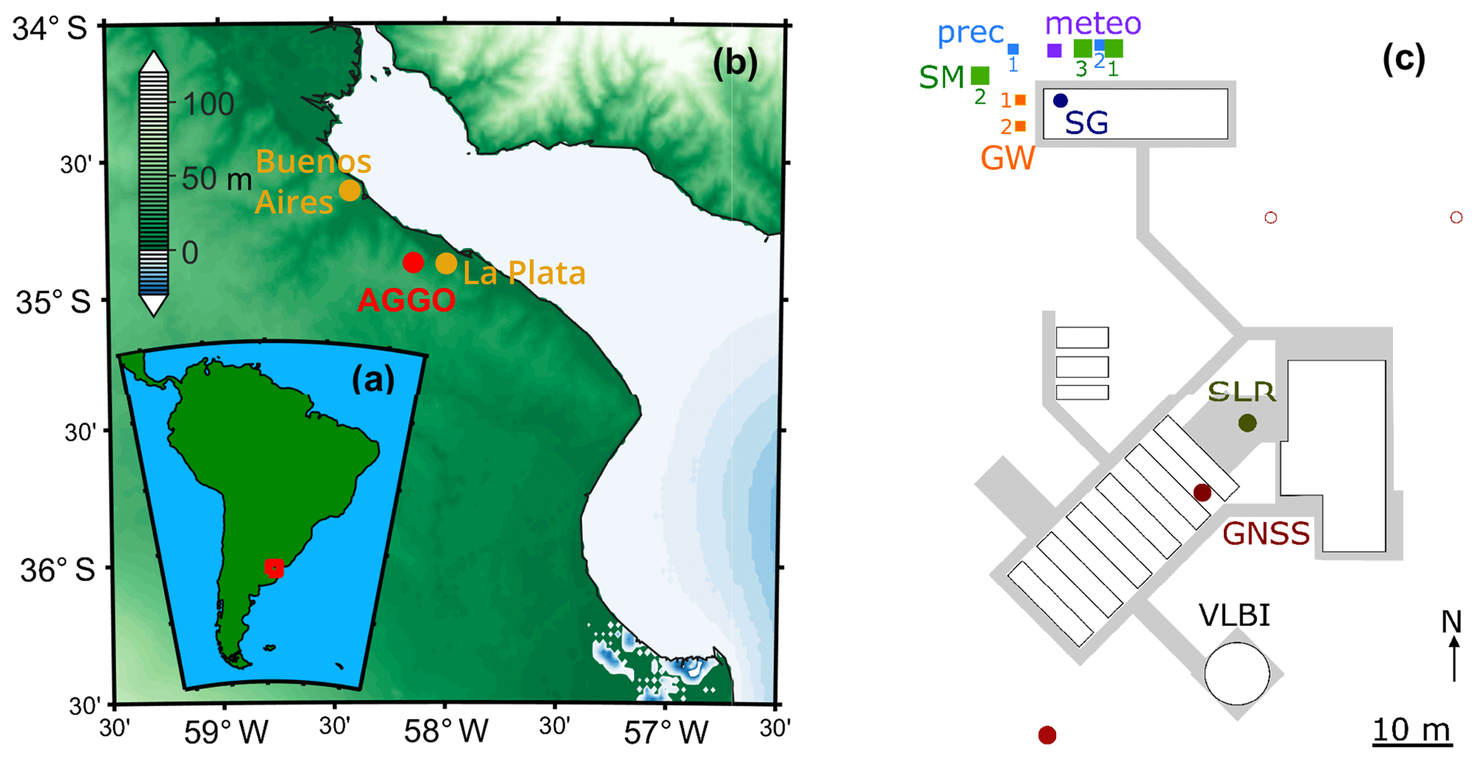
Figure 1Location of the study site (a, b, ϕ= 34∘52′24′′ S, λ= 58∘8′24′′ W). The local map (c on the right) shows the approximate instrumentation position (in colour), buildings as of April 2017 (white), and pavements (grey) at the AGGO site. Precipitation gauges (prec) in blue, soil pits for soil moisture (SM) sensors in green, weather station (meteo) in purple, superconducting gravimeter (SG) in dark blue, Global Navigation Satellite System (GNSS) antennas in red, groundwater (GW) observation wells in orange, and satellite laser ranging (SLR) station in dark green. The map was created using Amante and Eakins (2009), Wessel and Smith (1996), and M_Map toolbox (http://eoas.ubc.ca/~rich/map.html, last access: 2 November 2018).
The observatory was constructed on a plain formerly covered by eucalyptus trees. The eucalyptus forest still surrounds the majority of the area of the observatory. There are plans, however, to cut down the closest trees which could alter the hydrological regime in the future. The remaining area is covered by grassland, partially used as extensive pastureland. The observatory estate itself is predominately covered by grass with parts filled up with gravel. A geotechnical survey comprising three vertical profiles was carried out prior to the construction of the observatory. All profiles showed clayey soil (soil classification MH) with some calcareous layers up to a spatially varying depth of 3.9 to 6 m. Silty clayey to silty soils (class ML) were found up to the maximum depth of the borehole (10.2 m). The soil samples taken independently of the geotechnical survey for a laboratory analysis are summarized in Sect. 3.1.1 (Table 2).
The climate at AGGO can be classified according to Kottek et al. (2006) as Cfa (using Köppen–Geiger climate zone map; Rubel et al., 2017), i.e. humid subtropical climate. The long record from 1961 to 1990 at the meteorological station in La Plata (WMO station number 87593) processed by NOAA's National Climatic Data Center (ftp://ftp.atdd.noaa.gov/pub/GCOS/WMO-Normals, last access: 2 November 2018) shows daily mean temperature of 15.8 ∘C with mean maximum in January (22.6) and minimum in July (9.2). The mean annual relative humidity equals 77.2 % and the mean precipitation reaches 1007 mm. It should be noted that the distance between this meteorological station and AGGO is 24.2 km. Nonetheless, similar values (maximal difference of around 4 %) are observed at a site north-west of AGGO (36.5 km) in Buenos Aires (WMO station number 87576).
From a hydrogeological point of view, AGGO is located over the unconfined Pampeano aquifer (Pleistocene). The Pampeano formation has a thickness of about 30 m in this area and is composed predominantly of aeolian clayey to sandy silt (loess). Underlying the Pampeano is the semiconfined Puelche aquifer (early Pliocene), which is the main source of groundwater in the region. The Puelche formation is mostly of alluvial origin and it is formed by yellowish quartz sands, with local thin intercalations of gravels and/or clays. The contact between the Pampeano and Puelche formations is often marked by a silty clay layer that confines the Puelche aquifer. The regional groundwater flow of this aquifer system is toward the Río de La Plata estuary (zone of discharge) with very low hydraulic gradients.
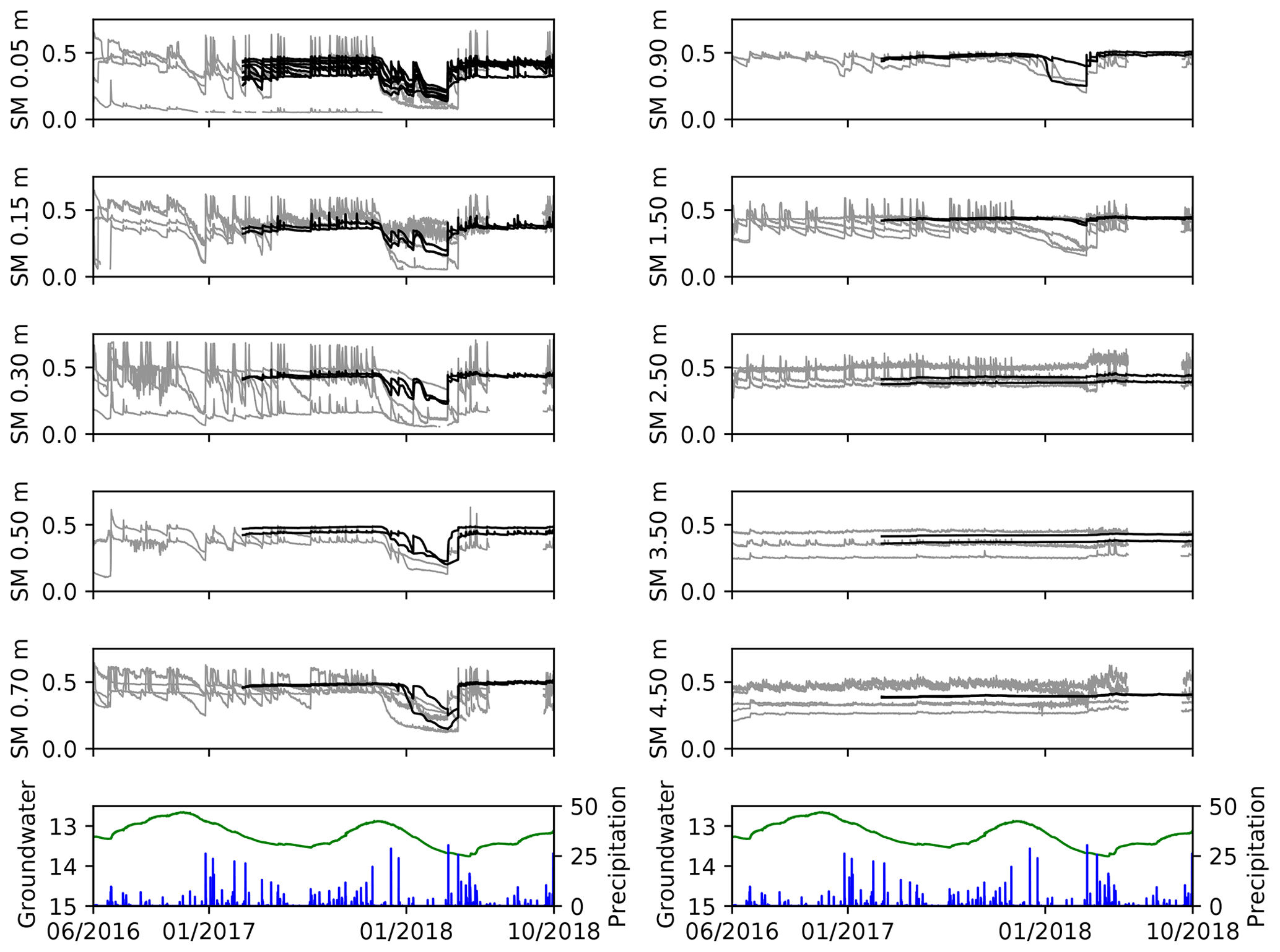
Figure 2All Level 2 soil moisture (SM) series at depths from 0.05 to 4.50 m in cubic metres per cubic metre, groundwater depth below land surface in metres, and precipitation (mm h−1). Soil moisture recorded with SMT100 sensors is in black; soil moisture recorded with TDR sensors is in grey and additionally filtered using a 13 h moving window.
The data set described here is available at https://doi.org/10.5880/GFZ.5.4.2018.001 (Mikolaj et al., 2018). The data set level indicates the degree of data modifications. Level 1 corresponds to the direct observations as collected by the sensors and written by the data logger. Except for the time-domain reflectometry (TDR) measurements, the Level 1 data are aggregations (mean or sum) of three previous measurements taken every 5 min. Level 2 comprises all Level 1 products after processing. The first step of the time series processing consists of removing values out of a plausible range. All missing data within a 1 h interval were then automatically filled by linear interpolation. If not stated otherwise (e.g. Sect. 3.1.2), longer gaps were not filled. Resulting values were used to compute either hourly means (e.g. soil moisture) or hourly sums (precipitation). Known issues or artificial signals were corrected by either interpolation or complete removal, depending on the length of the affected time period. In the last step of Level 2 processing, constant hourly sampling was enforced by flagging missing values. Information about the applied corrections along with system maintenance records, the local coordinates of the sensors, and installation notes are provided in separate relational tables of the data set.
The modelled data are denoted as Level 3 products. Provided are also the source code and the output of models that were created for this data set. Additional results of other models that were already available for AGGO are included in the data publication as well. Models specifically developed for this study include those for evapotranspiration, vadose zone water storage, combined precipitation series, and gravity effects. Globally available models used for large-scale gravity modelling were also exploited to extract air pressure, temperature, humidity, and water storage variation for the study sites. The maximal temporal coverage of the data set ranges from May 2016 up to November 2018 with some exceptions for sensors and models set up in May 2017.
3.1 Hydrological data
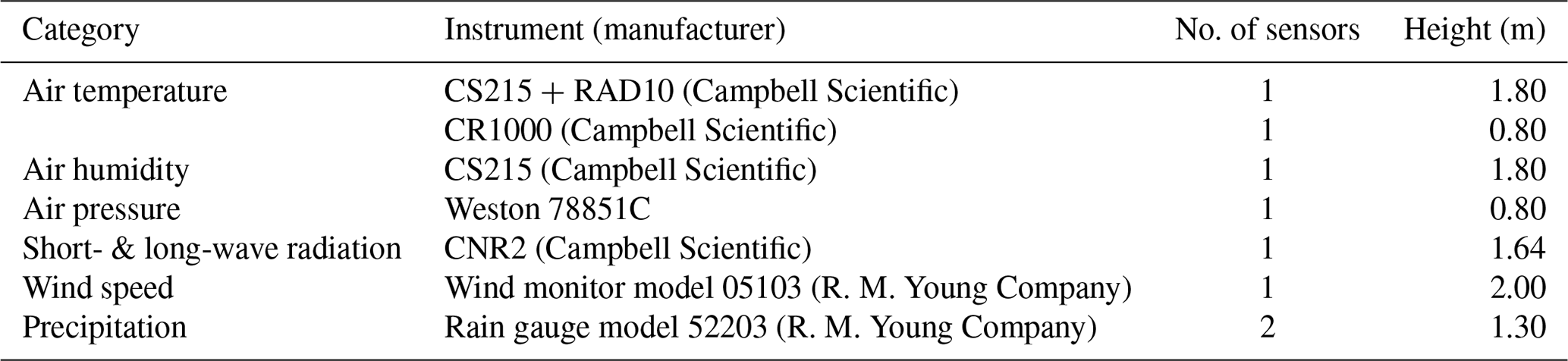
The spatial distribution of the hydrometeorological instrumentation is schematically shown in Fig. 1c. All sensors are located in the direct vicinity of the gravimeter building as observations by terrestrial gravimetry are known to be most sensitive to mass variations in the near field around the sensors (e.g. Güntner et al., 2017; Reich et al., 2018). Table 1 shows the type and the number of employed hydrological sensors. The accuracy of individual sensors under laboratory conditions can be found for some sensors in manufacturers' specifications (https://www.campbellsci.com/, http://www.youngusa.com/, https://www.ott.com/en-uk/, http://www.truebner.de/, http://www.gwrinstruments.com/index.html, last access: 6 November 2018). Actual accuracy is not provided here as it depends on several varying parameters such as length of sensor cables (e.g. for the TDR system), soil properties, or environmental temperature (e.g. for the SMT100 sensors). All sensors were deployed utilizing default manufacturer calibration and connected to one of the two data loggers (CR1000 by Campbell Scientific).
Table 1Hydrological instrumentation at AGGO.
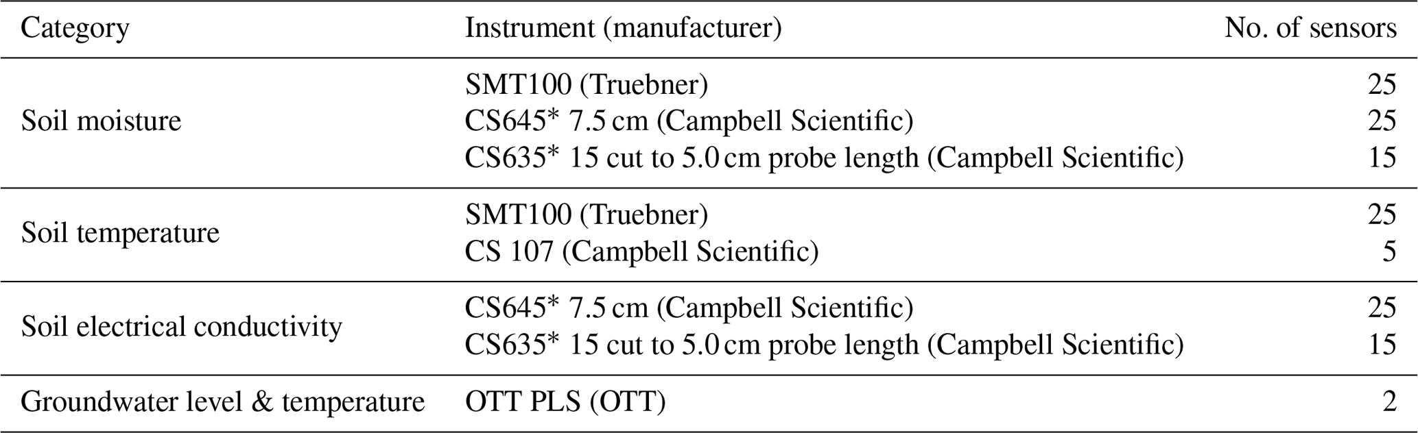
* Used in combination with TDR100 reflectometer and SDM8X50 multiplexer (Campbell Scientific).
3.1.1 Soil moisture, temperature, conductivity, and soil properties
A first set of soil moisture and soil electric conductivity sensors was installed at the AGGO site in April 2016. Time-domain reflectometry (TDR) sensors were deployed in two soil pits. Each pit was equipped with two profiles (SM 1 and 2 in Fig. 1c on the north and south sides of the pit). The manually dug pits allowed for installation of sensors up to a maximum depth of 4.5 m. Eight (or 10) sensors at 5, 15, 30, (50), 70, (90), 150, 250, 350, and 450 cm were distributed in each profile. Photographs of the installation campaign including the pits prior and after installation are part of the data publication. Due to the marked sensitivity of the TDR method to the high electric conductivity of the clayey soil, shortened CS635 sensors had to be used to minimize the travel distance of the electromagnetic pulse and to assure sufficient power of the reflected signal. Despite the reduced sensor length, these TDR measurements suffer from high noise, leading to a considerable number of data points out of a physically plausible range. Therefore, a third soil pit with two profiles was equipped with SMT100 soil moisture and temperature sensors in March 2017. These sensors show significantly less noise. Only 0.1 % of the SMT100 recordings are missing or are out of range, while almost 14 % of the data points recorded by the TDR system had to be discarded. Furthermore, all soil moisture time series should be treated with caution in the first couple of months after installation due to the soil compaction processes going on in the refilled soil pits in the direct vicinity of the sensors. The raw TDR measurements were converted to soil moisture according to Topp et al. (1980). In the case of the SMT100 sensors, the provided soil moisture output values relying on the manufacturer's calibration were directly taken. The soil moisture time series by TDR (grey) and SMT100 (black) sensors are shown in Fig. 2.
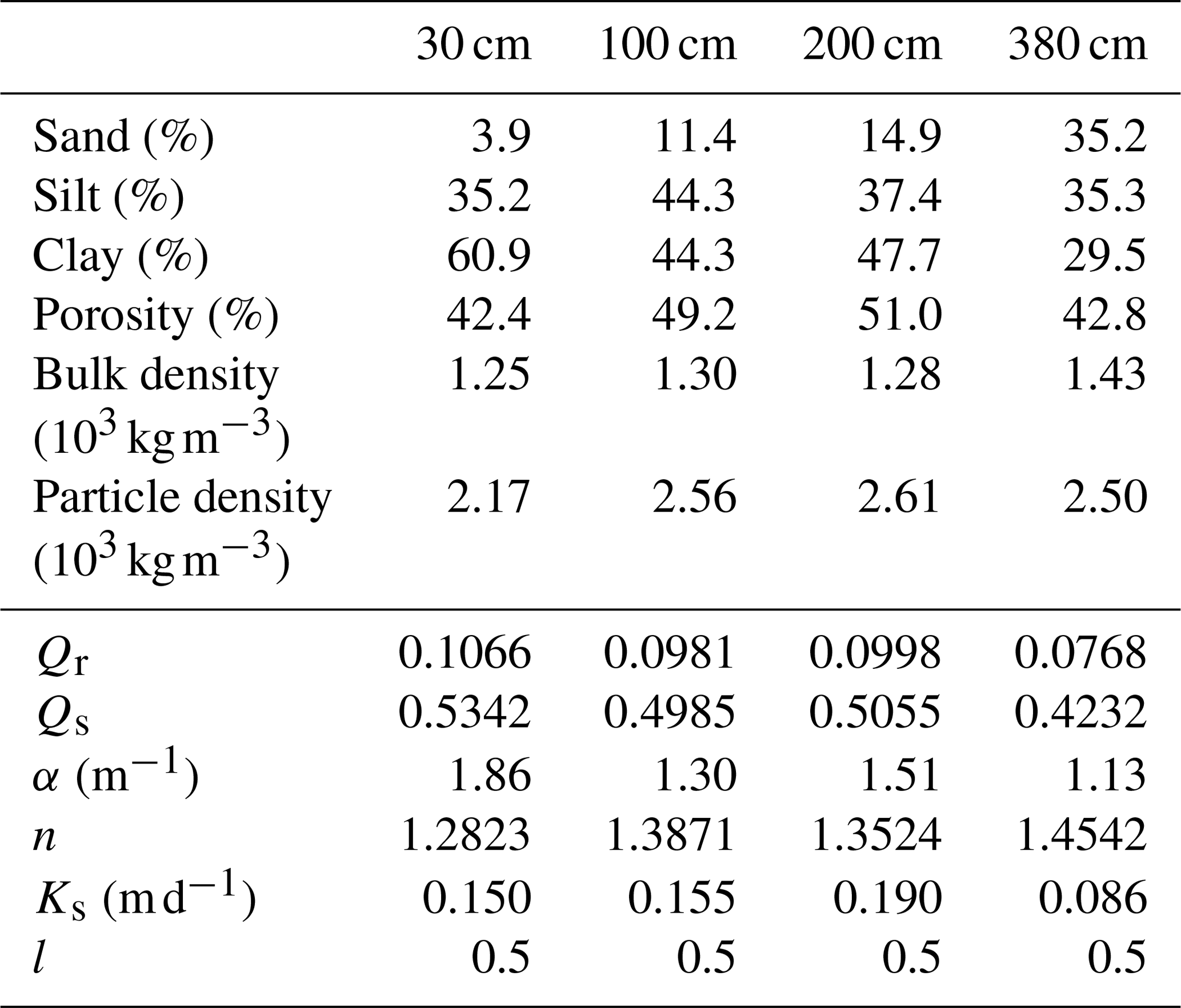
For characterization of soil physical parameters, four soil samples were taken for laboratory analysis at University of La Plata. All samples were taken from a soil pit that was later used for the gravimeter pillar, i.e. beneath the gravimeter building (location SG in Fig. 1c). The results of the analysis are shown in Table 2. The lower part of the table shows van Genuchten parameters estimated with the Rosetta Lite neural network prediction (Schaap et al., 2001) as implemented in the Hydrus-1D programme (http://pc-progress.com, last access: 28 November 2018).
The Hydrus-1D model (Šimůnek et al., 2016) was set up to quantify water storage variations in the vadose zone between the deepest soil moisture sensor at 4.5 m depth and the groundwater table. The soil hydraulic properties of the deepest soil sample were used for model parameterization. The upper time-variable boundary condition was set to the pressure head that corresponded to the mean of all variations observed at 4.5 m depth with the low-noise SMT100 sensors. All missing intervals were linearly interpolated to allow for one continuous model run. The lower boundary pressure head was given by the groundwater level observations described in the following section (Sect. 3.1.2). The first 3 weeks of the modelled soil moisture were removed to account for the spurious interval related to imperfect initial conditions. The resulting series are denoted as the Level 3 product sampled every 1.0 m between 5.5 and 11.5, and every 0.2 m between 12.1 and 12.5 m soil depth. Together with the other observation data of soil moisture and groundwater storage, the model output of vadose zone moisture obtained here allows for quantification of total water storage variations at the observatory. This is essential for modelling the gravity signals at the local scale (Sect. 3.3.2).
Table 2Soil physical properties and van Genuchten parameters for four AGGO soil samples at different depths.
3.1.2 Groundwater
Two groundwater wells were drilled at the observatory in April 2016 (see GW in Fig. 1c) and equipped with combined submerged pressure and temperature sensors for monitoring water level and temperature. The maximum depth of both wells is 33 m with their monitoring filter screen in between 16 and 32 m depth. The groundwater level and temperature observations reflect variations in the uppermost unconfined aquifer at the site, the Pampeano aquifer. The Level 1 groundwater series contain only 0.1 % missing values. The Level 2 groundwater level time series were corrected for pump tests and for any missing data points. Linear interpolation could be applied for this purpose due to the minimal noise and the absence of other short-term variations in the Level 1 time series. As shown in Fig. 2, a predominantly seasonal signal of groundwater levels can be observed, with an amplitude of about 1 m. The time series of both observation wells are close to identical with correlation r≈1.0 (p value ≈ 0.0) and a maximum difference of the Level 2 groundwater levels of 1 cm. This is related to the small distance of 3 m between both wells, designed for pump test experiments. Groundwater temperature was constant at 17.8 ∘C and no variations that exceeded the precision of the temperature sensor (±0.5 ∘C, https://www.ott.com/, last access: 6 November 2018) were observed during the study period.
In order to estimate the specific yield and other hydraulic parameters of the Pampeano aquifer a long-term pumping test was performed. The hydraulic test began on 15 May at 13:10 (UTC -3) and lasted until 17 May 2017 at 20:45 (UTC -3). During this period groundwater was pumped at an approximately constant rate of 6.1 m3 h−1 and water levels were measured in the two monitoring wells. Specific yield values that range from 0.085 to 0.10 were estimated for the Pampeano aquifer using different semi-analytical models implemented in the WTAQ computer programme described in Barlow and Moench (1999). As discussed and shown in Sect. 3.3.3 and Fig. 4, these estimations of specific yield are in good agreement with gravity residuals underlining the value of gravity observations for hydrogeological studies.
3.2 Meteorological data
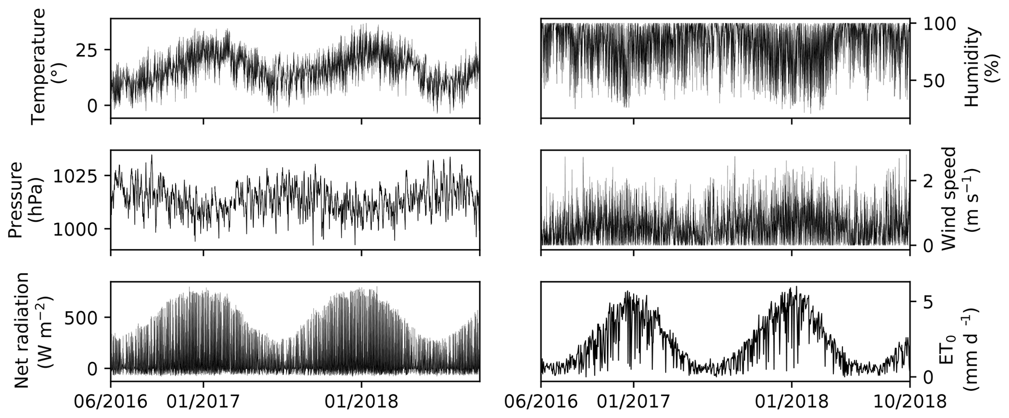
Table 3 presents an overview of the available meteorological instrumentation. All sensors except for the air pressure sensor have been in operation at AGGO since April 2016. All Level 1 time series show low noise and minimal missing data points equal to 0.2 % of the whole provided period (May 2016 to November 2018). The Level 3 products are without any missing data points. The Level 2 meteorological time series discussed in this section are shown in Fig. 3 (precipitation is shown in Fig. 2).
3.2.1 Air temperature, humidity, and pressure
The air temperature is recorded by two sensors (see Table 3). Only the CS215 sensor that is also used for relative humidity measurements is properly shielded against solar radiation. The ambient temperature recorded by the data logger sensor inside an enclosure attached to the pole of the meteorological station should be used only as a proxy in case the CS215 measurements are missing or corrupt. Both measurements are highly correlated (r=0.98, p value ≈ 0). Homogeneity tests carried out using the RHtest software package described in Wang and Feng (2013) and Wang (2008a, b) did not disclose any discontinuities (at α=0.05) in temperature, humidity, or pressure.
Unlike other meteorological instrumentation, the atmospheric pressure is recorded by a sensor installed inside the gravimeter building. The instrument was installed at AGGO together with the superconducting gravimeter in December 2015 (Wziontek et al., 2017). Provided here are hourly values starting on 1 January 2016 up to November 2018 (1.7 % missing data). The raw source data with 1 s and 1 min resolution can be obtained from the IGETS database hosted at the Information and Data Centre (http://isdc.gfz-potsdam.de, last access: 22 November 2018). The hourly values were linearly interpolated after applying a low-pass filter with a cutoff frequency of 2.6 h (at −3 dB) to the 1 min data.
Data series aggregated to daily values were compared to those of the two WMO sites that are closet to AGGO (WMO meteorological sites 87576 and 87593, https://www7.ncdc.noaa.gov/CDO/cdo, last access: 9 November 2018). Over 99.3 % of the variance in temperature series at all three locations can be explained by only one principle component. Also for air pressure and air humidity, the first component explains 99.8 % and 95.1 %, respectively. The clear dominance of large-scale atmospheric processes in the region can be furthermore highlighted by comparison to the ERA-Interim (Dee et al., 2011) global model. In this comparison, the correlation equals 0.94, 0.86, and 0.99 for temperature, humidity, and pressure, respectively (all p values ≈ 0.0). The acquisition of Level 3 model meteorological series is described in Sect. 3.3.2.
3.2.2 Wind speed, solar radiation, and precipitation
The net radiation at the site can be computed using provided solar shortwave and longwave radiation measured by sensors facing down- and upward. Radiation data are available in watts per square metre as 15 min (Level 1) or 60 min (Level 2) averages. The wind speed is measured at 2 m height but in proximity to a 4 m tall building. Furthermore, the distance to the eucalyptus trees is less than 10 m. These obstacles may limit the representativeness of these measurements to a small-scale area only. The correlation computed using daily mean time series of wind speed at AGGO and at the WMO stations 87576 and 87593 equals 0.66 and 0.60, respectively (both p values ≈ 0.0).
The liquid state precipitation at the observatory is recorded by two non-heated tipping-bucket rain gauges. The distance between the gauges is 10.9 m, while the shortest distance to the building equals 5 m. The distance to the tall eucalyptus trees is around 10 m. Related shielding effects may lead to under-catch of precipitation that is hard to quantify. Moreover, leaves and dirt cause occasional clogging of the instruments. These effects cause discrepancies between the two time series. A double mass technique disclosed several inhomogeneities. However, the plot of cumulative residuals against time and an associated ellipsis at α=0.05 after Allen and Smith (1998) (Annex 4) did not indicate overall inhomogeneity. The regression coefficient equals 0.83 and r2=0.68.
A Level 3 a continuous precipitation time series was created, addressing the discrepancies between both tipping-bucket records. The combination was performed manually by revising and replacing values of the first gauge by the second record at time intervals where the discrepancy exceeded 2 mm. In such cases, both WMO sites were used for comparison and for selection of those observations of the two AGGO rain sensors that resulted in closer agreement with the WMO precipitation series. The remaining missing records were set to zero.
Table 3Meteorological instrumentation with approximate height above surface.
3.2.3 Evapotranspiration
The grass reference evapotranspiration (ET0) was computed following the Penman–Monteith FAO-56 standard described in Allen and Smith (1998). Level 2 meteorological data were used as input for the computation. Hourly and daily ET0 estimates were computed separately using constants (Cd and Cn) tabulated in Allen et al. (2005). The daily values were checked against the estimates of the FAO ET0 Calculator (http://fao.org/land-water/databases-and-software/eto-calculator/en/, last access: 6 November 2018). It should be noted that the aggregated hourly values do not add up exactly to the independently computed daily rates. This is related to the inexact transformation of the equation parameters (e.g. Cd) as well as the inherently neglected hourly dynamics when exploiting the daily ET0 equation. For AGGO, the mean difference between aggregated hourly and daily values equals −0.18 mm d−1 (95 % rounded confidence interval −0.20 to −0.17 mm). Moreover, the null hypothesis of normally distributed differences can be rejected at α=0.05 using Anderson–Darling normality test (Stephens, 1974).
To comply with requirements of most hydrological models for continuous time series, the missing ET0 intervals were filled using the k-nearest-neighbour approach. Minimum and maximum daily temperature, dew point, and wind speed at the WMO La Plata 87593 site were used as proxies. A total of 80 % of the computed daily ET0 rates without missing intervals at AGGO were utilized for training. The remaining 20 % were used to find k with a minimal root-mean-square error of 0.87 mm d−1 (not rejecting the null hypothesis of normal distributed errors according to an Anderson–Darling test at α=0.05). The predicted daily ET0 rates were equally distributed over missing hourly intervals taking into account computed values if available for part of the affected day. Prior to the redistribution, missing intervals overnight (21:00 to 06:00 local time) were set to zero automatically.
3.3 Gravity
The data set contains gravity residuals corrected for tides, polar motion and length of day effects, local air pressure, and drift. Additional modelled gravity variations that aimed at further correction of the residuals for major environmental effects, such as global atmospheric, oceanic, and hydrological mass variations are provided as well. The input observed Level 1 gravity time series of the superconducting gravimeter at AGGO (Wziontek et al., 2017) can be accessed via the IGETS database. The IGETS database also provides Level 2 products (series-corrected instrumental issues ready for tidal analysis) processed by either the station operator or the University of French Polynesia (Voigt et al., 2016). The modelled series are divided into two main categories, depending on their respective integration radius of mass variations around the site. The local part refers to gravity effects arising from mass variation within an integration radius of 0.1∘ spherical distance following the approach of Mikolaj et al. (2015). Nonetheless, the source code provided along with the model outputs allows the user to modify the integration radius to any desired value. This also applies for the large-scale effects.
3.3.1 Gravity residuals
In this study, only Level 3 hourly gravity residuals are provided. These may differ from IGETS Level 3 products due to different processing strategies. For the computation of gravity residuals, the raw gravimeter signal was converted to units of gravity using a calibration factor of −736.5 and by applying a phase shift of −8.3 s. These parameters were estimated by using co-located absolute gravity measurements with a FG-5 gravimeter (calibration factor) and by evaluating the system response to an injected step function (phase shift). The 1 s gravity data were subsequently filtered and resampled to 1 min resolution. This gravity time series was then reduced for the effect of Earth and ocean tides applying parameters estimated in a tidal analysis carried out using ETERNA ET34-X-V61 (the updated version V71 is available at http://ggp.bkg.bund.de/eterna/, last access: 26 November 2018). Theoretical tides after Dehant et al. (1999) were used for long-periodic variations (fortnightly and longer). The polar motion and length of day variation were computed using the IERS EOP 14 C04 series (http://datacenter.iers.org, last access: 5 November 2018) after Torge (1989). The instrumental drift equal to 97.72 ± 3.51 was estimated using absolute gravimeter measurements carried out between January and June 2018. Due to the relatively short period between these absolute gravimeter observations, the drift estimate should be used with caution when studying long-term effects. A single admittance approach with −3 is used by default to correct the atmospheric effect. However, the residuals can be reduced for the global atmospheric effect discussed in the proceeding section (Sect. 3.3.2). The gravity time series was furthermore corrected for steps estimated by visual inspection and corrected for spurious time intervals by means of linear interpolations. Details on these corrections are in metadata tables. Finally, the time series was decimated to hourly temporal resolution by applying the identical low-pass filter as in the case of the Level 2 atmospheric pressure time series.
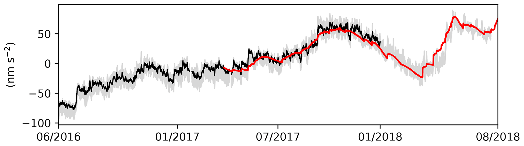
Figure 4Measured gravity residuals reduced for all available large-scale model combinations (in grey). Model combination Atmacs, ODT, and NOAH025 in black. Red line shows the local gravity model.
3.3.2 Large-scale model
The large-scale gravity effects are modelled taking into account atmospheric, hydrological, and non-tidal ocean mass transport. All hydrological effects are computed using the mGlobe toolbox described in Mikolaj et al. (2016). The input model data are listed in Table 4. The gravity effects were computed for an integration radius larger than 0.1∘, using all water storage compartments that were given by the individual models, mainly soil moisture up to a model-specific soil depth, and snow storage. The enforcement of mass conservation was implemented by applying a uniform layer over the ocean. The gravity response to such variation was computed assuming equal redistribution of model mass deficit or surplus compared to long-term mean. This approach did not take the mostly unreliable storage estimations over Antarctica and Greenland (set to zero). The global hydrological models were also exploited to obtain the Level 3 total water storage variations. It should be noted that none of these input models cover the whole saturated and unsaturated zone and should therefore be used accordingly.
The atmospheric effect was computed using three different input models. ERA-Interim was used in combination with the mGlobe toolbox (Mikolaj et al., 2016). The gravity effect corresponding to mass transport as modelled by ECMWF operational was directly obtained from EOST Loading Service (http://loading.u-strasbg.fr, last access: 8 October 2018). The third atmospheric model considered here was the ICON 384 global atmospheric model that is utilized in the Atmacs service for computing the gravity effect (http://atmacs.bkg.bund.de, last access: 8 October 2018). In addition to the atmospheric gravity effect, the model surface air pressure, humidity, and temperature were extracted to be used in the database (Level 3 products). For ERA-Interim, the time series were obtained using simple spatial linear interpolation. Atmacs provides only the model pressure at AGGO without need for spatial interpolation. In the case of the EOST products, the pressure time series were obtained after dividing the local contribution by a given conversion factor. The model pressure should be used in combination with in situ observations to refine the total atmospheric gravity effect as described in Mikolaj et al. (2016).
As shown in Oreiro et al. (2018), the effect of non-tidal ocean loading by storm surges plays a very important role in gravity recordings at AGGO. In this study, the corresponding gravity effect was computed using four models with global coverage. The ECCO1 (ECCO-JPL), ECCO2, and TUGOm gravity effects were downloaded from the EOST Loading Service (http://loading.u-strasbg.fr, last access: 8 October 2018). Additionally, the effect was computed by utilizing the OMCT RL06 model in combination with the mGlobe toolbox. The non-tidal loading effect of the Río de La Plata estuary was modelled after Oreiro et al. (2018). Like in the case of hydrological and atmospheric effects, the full spatial resolution of all input models was used for the computation.
The gravity effect was computed for all components using the highest available temporal resolution. The only exception was the hydrological effect where daily data were used. This simplification has a minimal effect on gravity as shown in Mikolaj et al. (2016). Hourly Level 3 time series provided in the database were obtained after linear interpolation. The comprehensive set of large-scale gravity effects allows for computation of gravity residuals reduced for global hydrological, atmospheric, and oceanic signals including minimum–maximum bounds. These bounds can be estimated by reducing the gravity residual for all possible combinations of available model. This approach presumes that the true large-scale gravity effect is not known and each model is treated as equally accurate. The result is shown in Fig. 4. In black are the residuals reduced for one particular model combination of large-scale effects, namely NOAH025, Atmacs, and the ODT model. The last model was chosen because of the efficient reduction of gravity effects of storm surges in the La Plata estuary. The residuals reduced for the large-scale gravity effects using all other model combinations are shown in grey (105 combinations in total). The uncertainty of large-scale gravity corrections as modelled in this study is discussed in Mikolaj et al. (2019).
Rodell et al. (2004)Mikolaj et al. (2016)Rodell et al. (2004)Mikolaj et al. (2016)Rodell et al. (2004)Mikolaj et al. (2016)Rodell et al. (2004)Mikolaj et al. (2016)Dee et al. (2011)Mikolaj et al. (2016)Gelaro et al. (2017)Mikolaj et al. (2016)Kanamitsu et al. (2002)Mikolaj et al. (2016)Zängl et al. (2014)Klügel and Wziontek (2009)Boy et al. (2009)Fukumori (2002)Boy et al. (2009)Menemenlis et al. (2008)Boy et al. (2009)Loren and Florent (2003)Boy et al. (2009)Dobslaw et al. (2017)Mikolaj et al. (2016)Oreiro et al. (2018)Oreiro et al. (2018)Table 4Large-scale gravity models for atmospheric (atmo), hydrological (hydro), non-tidal ocean (ntol), and estuary loading effects.
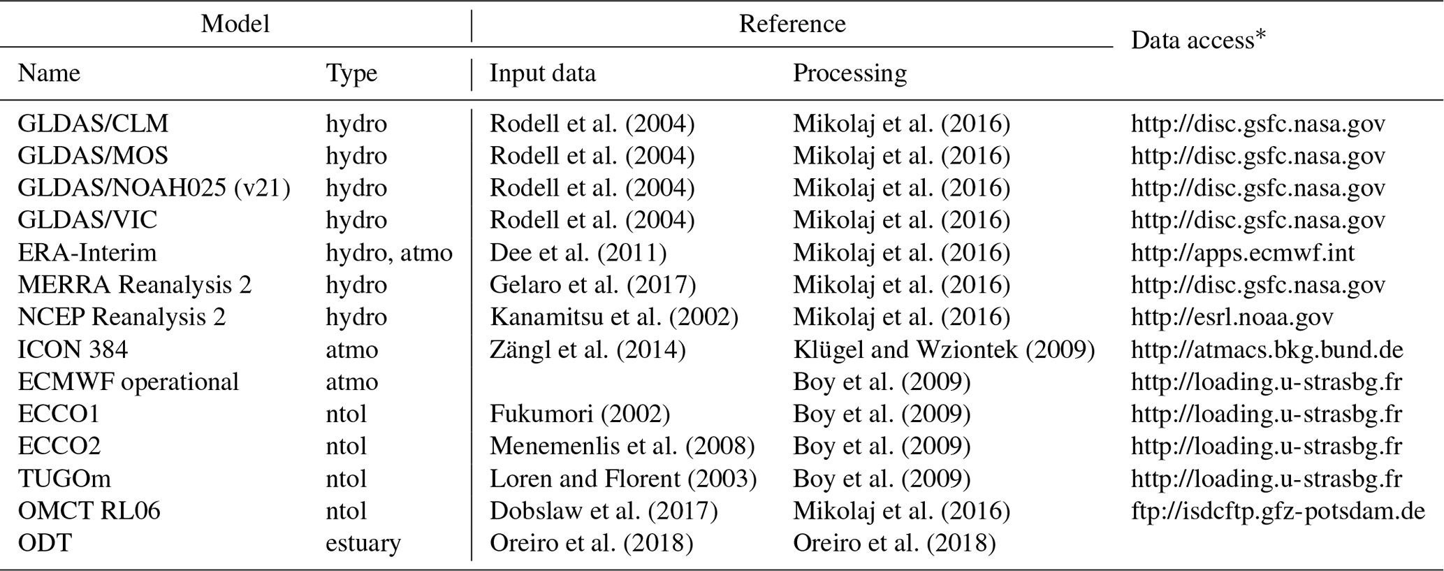
* Last access: 8 October 2018.
3.3.3 Local model
The local model of the water storage variations in the subsurface of the observatory extends the large-scale hydrological gravity models described in the previous section. Therefore, the local effect is computed for the whole area up to the integration radius of 0.1∘. However, in view of the minimal altitude variations in the study region and, thus, an assumption of a flat topography, only mass variations within approximately 100 m around the site efficiently contribute to the gravity effect (e.g. Güntner et al., 2017). In addition, soil moisture variations directly below the footprint of the gravimeter building were set to zero in accordance with Reich et al. (2018). Vertical discretization was set to fit the depth of the actual soil moisture measurements, i.e. with the first layer between 0.0 and 0.1 m up to the last layer between 4.0 and 5.0 m (see Sect. 3.1.1). A prism approximation was used for this purpose (Banerjee and Gupta, 1977). The low-noise Level 2 soil moisture time series collected by SMT100 sensors were used to compute the time-variable local gravity effect. The effect of groundwater storage variations was estimated by converting the groundwater level time series with a specific yield equal to 0.1 (10 %) as estimated in the pump test. The gravity effect of the vadose zone between the lowest soil moisture sensor and the groundwater level was quantified using the local hydrological model (HYDRUS-1D) described in Sect. 3.1.1. Resulting Level 3 local gravity effect time series were computed as the sum of all storage compartments, i.e. observation-based soil moisture, observation-constrained simulated vadose zone water storage, and observation-based groundwater storage variations. This composition allows for an independent validation of the hydrological products by comparing the result of the local gravity model to gravity residuals. As mentioned in the previous section, the gravity residuals need to be further reduced to signal corresponding to local hydrology by applying the aforementioned large-scale effects. The resulting gravity variations for one particular combination (NOAH025, Atmacs ODT) of large-scale effects is shown in Fig. 4 in black, while all other possible combinations are shown in grey. The red thick line corresponds to the local hydrological effect discussed in this section. The close correspondence of the resulting gravity residuals with the local hydrological gravity effect proves, on the one hand, the quality of the multi-compartmental data sets for gravity reductions based on local and global observations and models, and, on the other hand, the quality of the hydrometeorological monitoring system and its data set provided here for assessing the hydrological dynamics at AGGO.
The data set (Mikolaj et al., 2018, https://doi.org/10.5880/GFZ.5.4.2018.001) and code associated with the processing and modelling of the data (Mikolaj, 2018, https://doi.org/10.5880/GFZ.5.4.2018.002) are published via GFZ Data Services. The data set is organized in a database structure and prepared for implementation in a relational database. Nevertheless, all definitions and data tables are provided in separate text files allowing access without need for installation of a management system. However, the use of the relational database is advisable as it allows for easy access to all metadata information such as installation notes, sensor types, or applied reductions. The repository contains a set of example commands in MySQL. The processing scripts are written in Julia and MATLAB programming languages.
This study presents hydrological, meteorological, and gravity time series observed and modelled at the Argentine-German Geodetic Observatory (AGGO) between April 2016 and November 2018. Thanks to the existing and maintained infrastructure, the data set can be extended in the future to allow for studies of long-term variability and trends. Raw uncorrected, processed, and modelled series denoted as Level 1, 2, and 3 products, respectively, are provided. The directly observed series are suitable for users interested in observations that are not affected by any filtering and subjective data manipulation. Level 2 comprises time series corrected for instrumental and other issues while applying unified processing standards. The modelled series are tailored for studies where continuous homogenized inputs are needed. These may include hydrological modelling for water management or research purposes, verification of meteorological models, or use of gravity observations for interpretation of local geophysical phenomena. The gravity models are also of interest for studies aiming at evaluation of Gravity Recovery and Climate Experiment Follow On satellite mission via inter-comparisons to terrestrial observations. Furthermore, the presented data set directly feeds into the contributions of the AGGO observatory to realization and maintenance of regional- to global-scale terrestrial reference frames. The adequate consideration of local hydrological effects and loading-induced variations as provided in the study is required for this purpose.
MM drafted and coordinated the work on the paper, processed and modelled the time series, and compiled the database. AG, MR, and MM designed the hydrometeorological monitoring network at AGGO. AH, EA, HW, and FO contributed to data modelling. LG and JP conducted and evaluated the pump test. AP, AC, SS, AG, MR, and CB participated in instrument installation and contributed to the station maintenance. AG, CB, MG, and HW acquired project funds, supervised the project and revised the paper.
The authors declare that they have no conflict of interest.
The authors thank the whole AGGO staff for great support while setting up and maintaining the instrumentation. We also thank Mehedi Hasan (GFZ Potsdam) for helping with the SQL databases, Yang Feng for provision of the RHtest, and Klaus Schueller for further development of the ETERNA package. We also thank the anonymous reviewer for very constructive comments. We are deeply indebted to the Julia, Octave/MATLAB, and R developer community. Observed gravity time series and OMCT data used in this study were obtained from Information System and Data Center for geoscientific data servers at GFZ Potsdam. Selected gravity models were obtained from EOST Loading, and Atmacs services. The GLDAS and MERRA data sets used in this were acquired as part of the mission of NASA's Earth Science Division and archived and distributed by the Goddard Earth Sciences (GES) Data and Information Services Center (DISC). The ERA-Interim data used in this study were obtained from the ECMWF data server. The NCEP Reanalysis data were provided by the Physical Sciences Division of NOAA ESRL.
Compilation, processing, and publishing of the data set presented has been supported by the Bundesministerium für Bildung und Forschung (BMBF) and the Consejo Nacional de Investigaciones Científicas y Técnicas (CONICET) through the project “Hydrological and oceanic signals in geodetic observations at the Argentine–German Geodetic Observatory” (HOSGO) (grant no. 01DN16019).
This paper was edited by Birgit Heim and reviewed by Jeff Freymueller and two anonymous referees.
Allen, R. G., Pereira, L. S., Raes, D., and Smith, M.: Crop Evapotranspiration (guidelines for computing crop water requirements), FAO Irrigation and Drainage Paper No. 56, Tech. rep., Food and Agriculture Organization of the United Nations, 1998. a, b
Allen, R. G., Walter, I. A., Elliot, R. L., Howell, T. A., Itenfisu, D., Jensen, M. E., and Snyder, R.: The ASCE standardized reference evapotranspiration equation, Tech. rep., American Society of Civil Engineers Environmental and Water Resources Institute, 2005. a
Amante, C. and Eakins, B.: ETOPO1 1 Arc-Minute Global Relief Model: Procedures, Data Sources and Analysis. Technical Memorandum NESDIS NGDC-24, Report, NOAA National Geophysical Data Center, https://doi.org/10.7289/V5C8276M, 2009. a
Banerjee, B. and Gupta, S. P. D.: Gravitational attraction of a rectangular parallelepiped, Geophysics, 42, 1053–1055, https://doi.org/10.1190/1.1440766, 1977. a
Barlow, P. M. and Moench, A. F.: WTAQ – A computer program for calculating drawdowns and estimating hydraulic properties for confined and water-table aquifers, Tech. rep., US Geological Survey, 1999. a
Battaglia, M., Troise, C., Obrizzo, F., Pingue, F., and Natale, G. D.: Evidence for fluid migration as the source of deformation at Campi Flegrei caldera (Italy), Geophys. Res. Lett., 33, 1–4, https://doi.org/10.1029/2005gl024904, 2006. a
Boy, J.-P. and Hinderer, J.: Study of the seasonal gravity signal in superconducting gravimeter data, J. Geodyn., 41, 227–233, https://doi.org/10.1016/j.jog.2005.08.035, 2006. a
Boy, J.-P., Longuevergne, L., Boudin, F., Jacob, T., Lyard, F., Llubes, M., Florsch, N., and Esnoult, M.-F.: Modelling atmospheric and induced non-tidal oceanic loading contributions to surface gravity and tilt measurements, J. Geodyn., 48, 182–188, https://doi.org/10.1016/j.jog.2009.09.022, 2009. a, b, c, d
Braitenberg, C., Rossi, G., Bogusz, J., Crescentini, L., Crossley, D., Gross, R., Heki, K., Hinderer, J., Jahr, T., Meurers, B., and Schuh, H.: Geodynamics and Earth Tides Observations from Global to Micro Scale: Introduction, Pure Appl. Geophys., 175, 1595–1597, https://doi.org/10.1007/s00024-018-1875-0, 2018. a
Crossley, D. J., Boy, J.-P., Hinderer, J., Jahr, T., Weise, A., Wziontek, H., Abe, M., and Förste, C.: Comment on: “The quest for a consistent signal in ground and GRACE gravity time-series”, by Michel Van Camp, Olivier de Viron, Laurent Metivier, Bruno Meurers and Olivier Francis, Geophys. J. Int., 199, 1811–1817, https://doi.org/10.1093/gji/ggu259, 2014. a
Dee, D. P., Uppala, S. M., Simmons, A. J., Berrisford, P., Poli, P., Kobayashi, S., Andrae, U., Balmaseda, M. A., Balsamo, G., Bauer, P., Bechtold, P., Beljaars, A. C. M., van de Berg, L., Bidlot, J., Bormann, N., Delsol, C., Dragani, R., Fuentes, M., Geer, A. J., Haimberger, L., Healy, S. B., Hersbach, H., Hólm, E. V., Isaksen, L., Kȧllberg, P., Köhler, M., Matricardi, M., McNally, A. P., Monge-Sanz, B. M., Morcrette, J. J., Park, B. K., Peubey, C., de Rosnay, P., Tavolato, C., Thépaut, J. N., and Vitart, F.: The ERA-Interim reanalysis: configuration and performance of the data assimilation system, Q. J. Roy. Meteor. Soc., 137, 553–597, https://doi.org/10.1002/qj.828, 2011. a, b
Dehant, V., Defraigne, P., and Wahr, J. M.: Tides for a convective Earth, J. Geophys. Res.-Sol. Ea., 104, 1035–1058, https://doi.org/10.1029/1998JB900051, 1999. a
Dill, R. and Dobslaw, H.: Numerical simulations of global-scale high-resolution hydrological crustal deformations, J. Geophys. Res.-Sol. Ea., 118, 5008–5017, https://doi.org/10.1002/jgrb.50353, 2013. a
Dixon, T. H., Amelung, F., Ferretti, A., Novali, F., Rocca, F., Dokka, R., Sella, G., Kim, S.-W., Wdowinski, S., and Whitman, D.: Subsidence and flooding in New Orleans, Nature, 441, 587–588, https://doi.org/10.1038/441587a, 2006. a
Dobslaw, H., Bergmann-Wolf, I., Dill, R., Poropat, L., Thomas, M., Dahle, C., Esselborn, S., König, R., and Flechtner, F.: A new high-resolution model of non-tidal atmosphere and ocean mass variability for de-aliasing of satellite gravity observations: AOD1B RL06, Geophys. J. Int., 211, 263–269, https://doi.org/10.1093/gji/ggx302, 2017. a
Fukumori, I.: A Partitioned Kalman Filter and Smoother, Mon. Weather Rev., 130, 1370–1383, https://doi.org/10.1175/1520-0493(2002)130<1370:APKFAS>2.0.CO;2, 2002. a
Gelaro, R., McCarty, W., Suárez, M. J., Todling, R., Molod, A., Takacs, L., Randles, C. A., Darmenov, A., Bosilovich, M. G., Reichle, R., Wargan, K., Coy, L., Cullather, R., Draper, C., Akella, S., Buchard, V., Conaty, A., da Silva, A. M., Gu, W., Kim, G.-K., Koster, R., Lucchesi, R., Merkova, D., Nielsen, J. E., Partyka, G., Pawson, S., Putman, W., Rienecker, M., Schubert, S. D., Sienkiewicz, M., and Zhao, B.: The Modern-Era Retrospective Analysis for Research and Applications, Version 2 (MERRA-2), J. Climate, 30, 5419–5454, https://doi.org/10.1175/JCLI-D-16-0758.1, 2017. a
Güntner, A., Reich, M., Mikolaj, M., Creutzfeldt, B., Schroeder, S., and Wziontek, H.: Landscape-scale water balance monitoring with an iGrav superconducting gravimeter in a field enclosure, Hydrol. Earth Syst. Sci., 21, 3167–3182, https://doi.org/10.5194/hess-21-3167-2017, 2017. a, b
Heki, K. and Matsuo, K.: Coseismic gravity changes of the 2010 earthquake in central Chile from satellite gravimetry, Geophys. Res. Lett., 37, L24306, https://doi.org/10.1029/2010GL045335, 2010. a
Imanishi, Y., Sato, T., Higashi, T., Sun, W., and Okubo, S.: A Network of Superconducting Gravimeters Detects Submicrogal Coseismic Gravity Changes, Science, 306, 476–478, https://doi.org/10.1126/science.1101875, 2004. a
Kanamitsu, M., Ebisuzaki, W., Woollen, J., Yang, S.-K., Hnilo, J. J., Fiorino, M., and Potter, G. L.: NCEP-DOE AMIP-II Reanalysis (R-2), B. Am. Meteorol. Soc., 83, 1631–1644, https://doi.org/10.1175/BAMS-83-11-1631, 2002. a
Kennedy, J., Ferré, T. P. A., and Creutzfeldt, B.: Time-lapse gravity data for monitoring and modeling artificial recharge through a thick unsaturated zone, Water Resour. Res., 52, 7244–7261, https://doi.org/10.1002/2016WR018770, 2016. a
Klügel, T. and Wziontek, H.: Correcting gravimeters and tiltmeters for atmospheric mass attraction using operational weather models, J. Geodynam., 48, 204–210, https://doi.org/10.1016/j.jog.2009.09.010, 2009. a
Kottek, M., Grieser, J., Beck, C., Rudolf, B., and Rubel, F.: World Map of the Köppen-Geiger climate classification updated, Meteorol. Z., 15, 259–263, https://doi.org/10.1127/0941-2948/2006/0130, 2006. a
Loren, C. and Florent, L.: Modeling the barotropic response of the global ocean to atmospheric wind and pressure forcing-comparisons with observations, Geophys. Res. Lett., 30, 1275, https://doi.org/10.1029/2002GL016473, 2003. a
Menemenlis, D., Campin, J., Heimbach, P., Hill, C., Lee, T., Nguyen, A., Schodlok, M., and Zhang, H.: ECCO2: High Resolution Global Ocean and Sea Ice Data Synthesis, Mercator Ocean Quarterly Newsletter, 13–21, 2008. a
Mikolaj, M.: The processing and modelling of hydrometerological and gravity data at the Argentine-German Geodetic Observatory in La Plata, GFZ Data Services, https://doi.org/10.5880/GFZ.5.4.2018.002, 2018. a
Mikolaj, M., Meurers, B., and Mojzeš, M.: The reduction of hydrology-induced gravity variations at sites with insufficient hydrological instrumentation, Stud. Geophys. Geod., 59, 424–437, https://doi.org/10.1007/s11200-014-0232-8, 2015. a
Mikolaj, M., Meurers, B., and Güntner, A.: Modelling of global mass effects in hydrology, atmosphere and oceans on surface gravity, Comput. Geosci., 93, 12–20, https://doi.org/10.1016/j.cageo.2016.04.014, 2016. a, b, c, d, e, f, g, h, i, j, k, l
Mikolaj, M., Güntner, A., Brunini, C., Wziontek, H., Gende, M., Schröder, S., Pasquaré, A., Cassino, A. M., Reich, M., Hartmann, A., Oreiro, F. A., Pendiuk, J., Antokoletz, E. D., and Guarracino, L.: Hydrometerological and gravity data from the Argentine-German Geodetic Observatory in La Plata, GFZ Data Services, https://doi.org/10.5880/GFZ.5.4.2018.001, 2018. a, b, c
Mikolaj, M., Reich, M., and Güntner, A.: Resolving Geophysical Signals by Terrestrial Gravimetry: A Time Domain Assessment of the Correction-Induced Uncertainty, J. Geophys. Res.-Sol. Ea., 124, 2153–2165, https://doi.org/10.1029/2018JB016682, 2019. a
Oreiro, F. A., Wziontek, H., Fiore, M. M. E., D'Onofrio, E. E., and Brunini, C.: Non-Tidal Ocean Loading Correction for the Argentinean-German Geodetic Observatory Using an Empirical Model of Storm Surge for the Río de la Plata, Pure Appl. Geophys., 175, 1739–1753, https://doi.org/10.1007/s00024-017-1651-6, 2018. a, b, c, d, e, f
Reich, M., Mikolaj, M., Blume, T., and Güntner, A.: Reducing gravity data for the influence of water storage variations beneath observatory buildings, Geophysics, 1–81, https://doi.org/10.1190/geo2018-0301.1, 2018. a, b
Rodell, M., Houser, P. R., Jambor, U., Gottschalck, J., Mitchell, K., Meng, C. J., Arsenault, K., Cosgrove, B., Radakovich, J., Bosilovich, M., Entin, J. K., Walker, J. P., Lohmann, D., and Toll, D.: The Global Land Data Assimilation System, B. Am. Meteorol. Soc., 85, 381–394, https://doi.org/10.1175/BAMS-85-3-381, 2004. a, b, c, d
Rubel, F., Brugger, K., Haslinger, K., and Auer, I.: The climate of the European Alps: Shift of very high resolution Köppen-Geiger climate zones 1800–2100, Meteorol. Z., 26, 115–125, https://doi.org/10.1127/metz/2016/0816, 2017. a
Sánchez, L., Drewes, H., Brunini, C., Mackern, M. V., and Martínez-Díaz, W.: SIRGAS Core Network Stability, in: International Association of Geodesy Symposia, Springer International Publishing, 183–191, https://doi.org/10.1007/1345_2015_143, 2015. a
Sato, T., Boy, J. P., Tamura, Y., Matsumoto, K., Asari, K., Plag, H.-P., and Francis, O.: Gravity tide and seasonal gravity variation at Ny-Ȧlesund, Svalbard in Arctic, J. Geodynam., 41, 234–241, https://doi.org/10.1016/j.jog.2005.08.016, 2006. a
Schaap, M. G., Leij, F. J., and van Genuchten, M. T.: Rosetta: a computer program for estimating soil hydraulic parameters with hierarchical pedotransfer functions, J. Hydrol., 251, 163–176, https://doi.org/10.1016/S0022-1694(01)00466-8, 2001. a
Šimůnek, J., van Genuchten, M. T., and Šejna, M.: Recent Developments and Applications of the HYDRUS Computer Software Packages, Vadose Zone J., 15, 1–25, https://doi.org/10.2136/vzj2016.04.0033, 2016. a
Stephens, M. A.: EDF Statistics for Goodness of Fit and Some Comparisons, J. Am. Stat. Assoc., 69, 730–737, https://doi.org/10.1080/01621459.1974.10480196, 1974. a
Topp, G. C., Davis, J. L., and Annan, A. P.: Electromagnetic determination of soil water content: Measurements in coaxial transmission lines, Water Resour. Res., 16, 574–582, https://doi.org/10.1029/WR016i003p00574, 1980. a
Torge, W.: Gravimetry, Walter de Gruyter, Berlin, 1989. a
Van Camp, M., de Viron, O., Métivier, L., Meurers, B., and Francis, O.: The quest for a consistent signal in ground and GRACE gravity time-series, Geophys. J. Int., 197, 192–201, https://doi.org/10.1093/gji/ggt524, 2014. a
Voigt, C., Förste, C., Wziontek, H., Crossley, D., Meurers, B., Pálinkáš, V., Hinderer, J., Boy, J.-P., Barriot, J.-P., andSun, H.: Report on the Data Base of the International Geodynamics and Earth Tide Service (IGETS), Tech. rep., GFZ Potsdam, https://doi.org/10.2312/GFZ.b103-16087, 2016. a, b
Wang, X. L.: Accounting for Autocorrelation in Detecting Mean Shifts in Climate Data Series Using the Penalized Maximal t or F test, J. Appl. Meteorol. Climatol., 47, 2423–2444, https://doi.org/10.1175/2008jamc1741.1, 2008a. a
Wang, X. L.: Penalized Maximal F Test for Detecting Undocumented mean Shift without Trend Change, J. Atmos. Ocean. Tech., 25, 368–384, https://doi.org/10.1175/2007jtecha982.1, 2008b. a
Wang, X. L. and Feng, Y.: RHtestsV4 User Manual, Tech. rep., Climate Research Division, Atmospheric Science and Technology Directorate, Science and Technology Branch, Environment Canada, http://etccdi.pacificclimate.org/software.shtml (last access: 2 October 2018), 2013. a
Wessel, P. and Smith, W. H. F.: A global, self-consistent, hierarchical, high-resolution shoreline database, J. Geophys. Res., 101, 8741–8743, 1996. a
Wilson, C. R., Scanlon, B., Sharp, J., Longuevergne, L., and Wu, H.: Field Test of the Superconducting Gravimeter as a Hydrologic Sensor, Groundwater, 50, 442–449, https://doi.org/10.1111/j.1745-6584.2011.00864.x, 2011. a
Wziontek, H., Wolf, P., Häfner, M., Hase, H., Nowak, I., Rülke, A., Wilmes, H., and Brunini, C.: Superconducting Gravimeter Data from AGGO/La Plata – Level 1, https://doi.org/10.5880/igets.lp.l1.001, 2017. a, b
Zängl, G., Reinert, D., Rípodas, P., and Baldauf, M.: The ICON (ICOsahedral Non-hydrostatic) modelling framework of DWD and MPI-M: Description of the non-hydrostatic dynamical core, Q. J. Roy. Meteor. Soc., 141, 563–579, https://doi.org/10.1002/qj.2378, 2014. a