the Creative Commons Attribution 4.0 License.
the Creative Commons Attribution 4.0 License.
 | 13 Nov 2019
GRUN: an observation-based global gridded runoff dataset from 1902 to 2014
Vincent Humphrey
Sonia I. Seneviratne
Lukas Gudmundsson
Freshwater resources are of high societal relevance, and understanding their past variability is vital to water management in the context of ongoing climate change. This study introduces a global gridded monthly reconstruction of runoff covering the period from 1902 to 2014. In situ streamflow observations are used to train a machine learning algorithm that predicts monthly runoff rates based on antecedent precipitation and temperature from an atmospheric reanalysis. The accuracy of this reconstruction is assessed with cross-validation and compared with an independent set of discharge observations for large river basins. The presented dataset agrees on average better with the streamflow observations than an ensemble of 13 state-of-the art global hydrological model runoff simulations. We estimate a global long-term mean runoff of 38 452 km3 yr−1 in agreement with previous assessments. The temporal coverage of the reconstruction offers an unprecedented view on large-scale features of runoff variability in regions with limited data coverage, making it an ideal candidate for large-scale hydro-climatic process studies, water resource assessments, and evaluating and refining existing hydrological models. The paper closes with example applications fostering the understanding of global freshwater dynamics, interannual variability, drought propagation and the response of runoff to atmospheric teleconnections. The GRUN dataset is available at https://doi.org/10.6084/m9.figshare.9228176 (Ghiggi et al., 2019).
- Article
(11744 KB) -
Supplement
(3603 KB) - BibTeX
- EndNote


Water is one of the most important natural resources for human development and its availability affects water supplies, agricultural yields, energy production, and infrastructure safety and operation. Two-thirds of the global population is currently exposed to severe water scarcity (Vörösmarty et al., 2010; Kummu et al., 2016; Mekonnen and Hoekstra, 2016), and a recent annual risk report of the World Economic Forum (WEF, 2018) lists the water crisis as one of the largest global risks in terms of potential impact and likelihood. While river flow is regularly used to assess regional renewable freshwater resources (Vörösmarty et al., 2000; Oki and Kanae, 2006; Veldkamp et al., 2017; Munia et al., 2018), there is to date no publicly available global dataset providing observation-based estimates of the evolution of runoff and river flow throughout the 20th and the early 21st centuries. In the last decades, several international initiatives promoted the launch of modelling inter-comparison projects with the aim to improve the representation of the terrestrial water cycle in global hydrological models (Dirmeyer et al., 2006; Dirmeyer, 2011; Haddeland et al., 2011; Harding et al., 2011; Van Den Hurk et al., 2011; Warszawski et al., 2014; Van Den Hurk et al., 2016; Schellekens et al., 2017) as well as to develop tools to refine regional hydrological predictions in data-sparse regions (Sivapalan, 2003; Blöschl et al., 2013; Hrachowitz et al., 2013). In the meantime, a widespread decline in the number of streamflow monitoring stations has also been reported (Shiklomanov et al., 2002; Fekete and Vörösmarty, 2007; Fekete et al., 2012, 2015; Laudon et al., 2017) and alternative estimates of streamflow are thus needed for reconstructing past large-scale runoff variability, not only during the beginning of the century but also in recent decades.
In this contribution, we use a recently published collection of in situ streamflow data (Do et al., 2018; Gudmundsson et al., 2018b) in combination with a century-long reanalysis (Compo et al., 2011; Kim et al., 2017) to fill this gap. This study introduces a global gridded reconstruction of monthly runoff covering the period from 1902 to 2014 at a 0.5∘ spatial resolution. Runoff is defined here as the amount of water drained from a given land unit (i.e. grid cell) eventually entering the river system, including groundwater flow and snowmelt. The methodology builds upon previous work where gridded runoff rate estimates were obtained for Europe (Gudmundsson and Seneviratne, 2015, 2016). Hereafter, these two papers are referred to as GS15 and GS16. Monthly observations of precipitation, temperature and observed runoff rates from small catchments are used as input for a machine learning (ML) algorithm to learn the runoff generation process without the explicit description of the involved hydrological processes. Gridded precipitation and temperature data are then used to predict runoff rates in ungauged regions as well. The reconstruction accuracy is evaluated using runoff observations at the grid-cell scale as well as river discharge measurements in large river basins, both not used for model training. It is also benchmarked against an ensemble of global hydrological model simulations forced with the same precipitation and temperature data.
The paper concludes with a section illustrating the potential of the newly established data product (GRUN) for climatological, hydrological and environmental studies.
2.1 Modelling data
2.1.1 Atmospheric forcing
Gridded observations of precipitation and temperature data are obtained from the Global Soil Wetness Project Phase 3 (GSWP3) dataset (version 1.05) (Kim et al., 2017). GSWP3 is a dynamically downscaled and bias-corrected version of the 20th Century Reanalysis (20CR) (Compo et al., 2011). The dataset covers the period 1901 to 2014 and is available on a regular grid at 3-hourly resolution. The sub-daily data are aggregated to monthly means and bilinearly interpolated to a cylindrical equal-area (CEA) grid composed of cells with an area of 2500 km2 and a spatial resolution of approximately 50 km.
2.1.2 Runoff observations
Monthly runoff observations are derived from the Global Streamflow Indices and Metadata Archive (GSIM) (Do et al., 2018; Gudmundsson et al., 2018b). This dataset includes a collection of 35 002 streamflow stations obtained by merging existing international and national databases. GSIM provides a wide range of time series indices at monthly, seasonal and yearly resolution. Here time series of monthly mean streamflow are considered. The data selection and preprocessing of these observations is detailed in Sect. 3.1.
2.2 Validation data
2.2.1 Observed continental-scale river discharge
Observed monthly river discharge from 718 large river basins is taken from the Global Runoff Data Centre (GRDC) Reference Dataset (https://www.bafg.de/GRDC/EN/04_spcldtbss/43_GRfN/refDataset_node.html, last access: 31 October 2019). The dataset contains a selection of streamflow stations with a basin area greater than 10 000 km2 and corresponding catchment shapefiles. These time series are removed from GSIM to ensure that independent observations are used for model evaluation (see Sect. 3.3).
2.2.2 Global hydrological models' simulations
The Inter-Sectoral Impact Model Intercomparison Project (ISIMIP) offers a framework to compare simulations and to quantify the uncertainty across hydrological and land surface models forced with equal inputs (Warszawski et al., 2014). The accuracy of GRUN is benchmarked against runoff simulations for the period 1971–2010 from an ensemble of state-of-the-art global hydrological models (GHMs) participating in the second phase of ISIMIP2a Water (Gosling et al., 2017). The GHM simulations used in the main text are driven with the GSWP3 forcing and do not account for human impacts on river flow (“nosoc” scenario). In the Supplement, we also provide the results based on simulations that account for direct human impacts (i.e. the “pressoc” and “varsoc” scenarios from ISIMIP2a). Further details on the ISIMIP2a simulation setup can be found at https://www.isimip.org/protocol/#isimip2a (last access: 31 October 2019).
3.1 GSIM time series selection and preprocessing
Step 1. Sub-setting GSIM stations and conversion of flow volumes to runoff rates
Runoff is defined here as all the water draining from a small land area. Runoff cannot be observed directly, but at a monthly timescale the average catchment runoff can be assumed to equal the monthly streamflow measured at the outlet divided by the catchment area, provided storage of river water (e.g. in dams, reservoirs) and/or river water losses (e.g. river channel and lake evaporation, irrigation) are minimal. Thus, runoff rates (millimetres per month) are obtained by dividing the GSIM river discharge (cubic metres per month) with the station's upstream catchment area (km2). We then select catchments with an area comparable to the grid-cell size of the atmospheric forcing data in order to derive observational estimates of the runoff rate response to changes in atmospheric forcing.
To retrieve accurate estimates of grid-cell runoff, only GSIM stations fulfilling the following criteria have been selected for further analysis.
-
The time series has observations within the period 1902–2014 (when GSWP3 forcing is available).
-
The original data provider reports an estimate of the drainage area. This choice is made to have the possibility to verify the geographic location of the station as well as to assess the reliability of the automated delineation of the drainage area using a digital elevation model as provided in GSIM (Do et al., 2018).
-
GSIM provides the shape of the drainage area and the quality of the catchment delineation is flagged as “medium” or “high”. This criterion imposes that the difference between the drainage area reported by the data provider and the one estimated by GSIM is less than 10 % (Do et al., 2018).
-
The drainage area is between 10 and 2500 km2. Very small catchments (<10 km2) are discarded because the uncertainty in the drainage area can significantly affect the magnitude of the runoff rates. On the other hand, catchments larger than 2500 km2 are removed because their drainage area spans too many grid cells of the atmospheric forcing.
Based on these criteria, 10 042 GSIM stations are selected for further analysis.
Step 2. Correction for mislabelled missing values
Manual investigation of monthly river discharge time series revealed the occurrence of multiple consecutive months with streamflow volumes exactly equal to 0 m3 per month, in disagreement with the observed regional runoff pattern. These artefacts likely stem from a misleading treatment of missing values (e.g. due to damaged sensors). To identify such likely missing values, all time series are screened for the presence of more than 3 consecutive months with values of zero. If this pattern occurs, all zero values in the monthly time series are set to “missing”.
Step 3. Remove time series with unrealistic runoff rates and short temporal coverage
The following criteria have been adopted to remove observations that are too sparse or physically very unlikely:
-
Remove time series with only missing values.
-
Remove time series with negative monthly runoff rates.
-
Remove time series with less than 2 years of observations.
-
Remove time series with monthly runoff rates higher than 2000 mm per month.
This screening step gives a selection of 8211 stations.
Step 4. Homogeneity testing
River discharge time series can show temporal changes in the hydrological behaviour because of changing instrumentation, recalibration of streamflow rating curves, flow regulation (i.e. dam construction) and other human activities (i.e. irrigation). Automated identification of such break points is usually done using statistical tests (Gudmundsson et al., 2018b). GSIM used a general-purpose procedure that was applied to all indices/timescales. In this study, the following two target-oriented change-point detection methods are applied after log-transformation of the time series:
-
univariate normal change point in mean (Chen and Gupta, 2012);
-
univariate normal change point in variance (Chen and Gupta, 2012);
-
univariate normal change point in normal mean and variance (Chen and Gupta, 2012).
Runoff time series are discarded when any of these tests detects a change point.
Figure 1 shows three river flow time series with different types of detected change points. Figure 1a illustrates the ability of the tests to identify gradual changes in low flow regulation or low flow measurement precision. Figure 1b displays the detection of sudden changes in the mean of the time series, e.g. caused by dam construction, river diversion or measurement errors, while Fig. 1c shows the potential in spotting subtle changes in river discharge variability possibly induced by reservoir operations.

Figure 1Detection of change points in runoff time series. The vertical red line indicates the change point in variance detected by the univariate normal change point in variance test, while the horizontal blue dashed lines illustrate the change in mean identified by the test of univariate normal change point in normal mean and variance. The title of the individual panels corresponds to the station identifier as used in GSIM.
The homogeneity testing procedure resulted in a final selection of 7264 stations.
The file “GSIM_training_stations.csv” provided in the Supplement lists this subset of GSIM stations, while Fig. S1 in the Supplement shows the catchment area distribution of these stations.
3.2 Retrieving runoff rates at the grid-cell scale of atmospheric forcing data
To give equal importance to high-latitude and tropical observations, the entire modelling procedure is conducted on a cylindrical equal-area (CEA) grid composed of cells with an area of 2500 km2 and a spatial resolution of approximately 50 km. The final gridded runoff product is however projected back onto the WGS84 grid of the atmospheric forcing data.
Because of the high density of stations in some regions and the typically elongated shape of the drainage area, many runoff observations span multiple cells of the CEA grid. Thus, an observational runoff time series representative of each cell is retrieved as follows:
-
project the GSIM catchment shape to the CEA grid, and
-
for each grid cell
- a.
select those catchments of which the drainage area intersects the grid cell, and
- b.
at each time step, take the median runoff rate of the selected catchments.
- a.
In addition to reducing the oversampling in high-station-density regions, this preprocessing step also smooths out some sub-grid variability. Additionally, it can also reduce the effect of potential outliers (i.e. stations that have exceptionally high or low runoff rates compared to their neighbours). To avoid inhomogeneities arising from the concatenation of different runoff time series, the observational runoff time series at each grid cell is submitted to another homogeneity testing run (as described in Sect. 3.1, step 4). The procedure resulted in 5094 grid cells usable for model training, covering 8.5 % of the total land area and yielding 2 703 902 monthly runoff rate observations. Hereinafter, the grid-cell runoff time series are referred to as the runoff observations and Fig. 2 shows their spatio-temporal coverage.
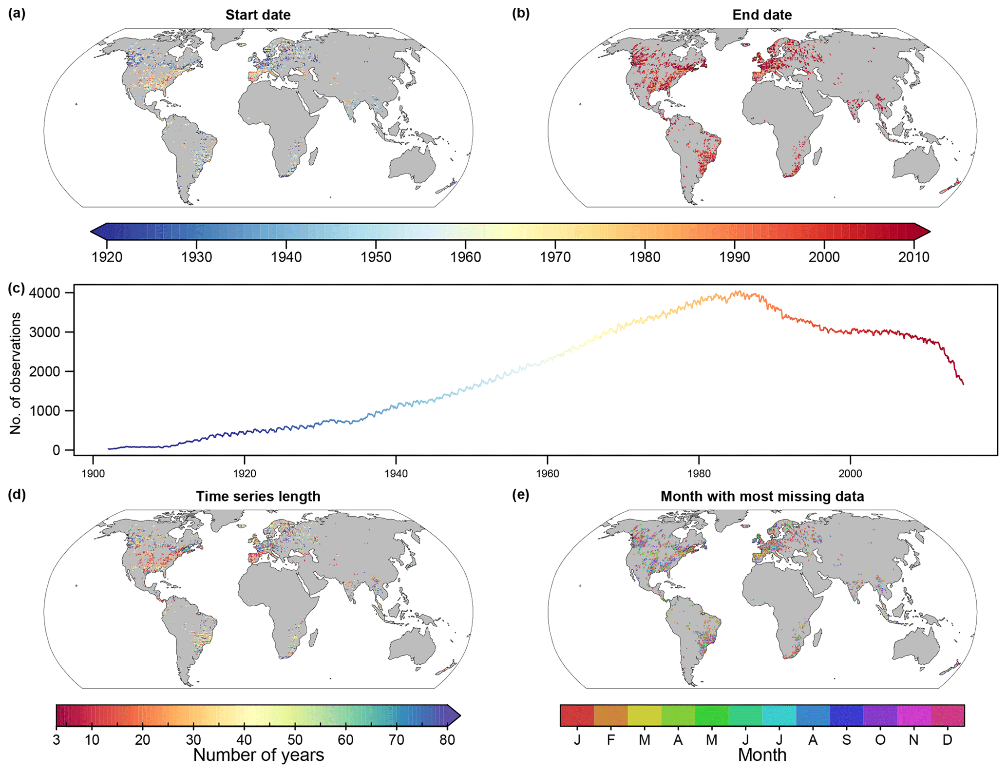
Figure 2Spatio-temporal coverage of grid-cell runoff observations. Panels (a) and (b) display the start and end year of the time series respectively. (c) Total number of runoff observations at each month between 1902 and 2014. (d) Number of years with at least 10 runoff observations in each year. (e) Month with most missing values.
3.3 Selection and preprocessing of GRDC time series
To obtain an independent dataset for assessing the accuracy of GRUN in large river basins, streamflow stations with a catchment area larger than 10 000 km2 are selected from the GRDC reference dataset. Although most of these stations are included in the GSIM collection, they are not used for model training because only catchments with an area smaller than 2500 km2 are used to derive grid-cell runoff observations (Sect. 3.1, step 1).
The GRDC time series are subject to the preprocessing steps 1 to 4 detailed in Sect. 3.1 to discard streamflow records of low quality. This procedure results in a selection of 379 large river basins.
4.1 Model setup
For the first time, GS15 and GS16 have used a ML algorithm to estimate monthly runoff at continental scale, and Ghiggi (2018) explored the utility of a wide range of algorithms to improve the task. Based on these findings, the present study employs the random forest (RF) algorithm (Breiman, 2001). RF is a ML algorithm which averages a set of randomized regression trees (Breiman et al., 1984) trained on different subsets of the original data. A regression tree divides the predictor space into high-dimensional rectangles by means of recursive binary splits. The predicted value of a new observation is the average of the observations used in the training process located in the region of the predictor space to which the new predictor values belong. By averaging the predictions of several randomized regression trees built on different training data, RF improves the final accuracy of the runoff estimates.
The monthly runoff rate (R) is modelled as a function of monthly precipitation (P) and monthly near-surface temperature (T) as
where f corresponds to the RF model (RFM), s represents the identifier of the CEA grid cell, t is the time step, and τ is a time lag operator that provides information about meteorological conditions of the past 6 months to allow the RFM to approximate water storage effects that influence the runoff generation process. This differs from GS15 and GS16, which used a time lag operator of 12 months. The reasons behind this change are a reduction in training time of RFM and a decrease in collinearity between predictors (caused by the seasonal cycle).
Both precipitation and runoff observations are log-transformed before model training to adjust the skewed distribution of the data and to avoid only a small number of high-flow events dominating the optimization of the squared error loss. Once the RFM is trained, gridded precipitation and temperature data are fed to the model to obtain the final runoff reconstruction. Finally, the log-transformation of the predicted runoff values is inverted to derive runoff rates in conventional units.
The decision to only consider precipitation and temperature as explanatory variables is motivated by GS15, who found that the inclusion of other atmospheric variables as well as selected land parameters (topography and soil texture) did not significantly improve the overall accuracy of the estimate. Furthermore, reducing the number of predictor variables also helped to reduce computational costs significantly. While a more extensive screening of other land parameters is beyond the scope of this study, this could be the subject of potential future research.
4.2 The GRUN reconstruction
Accurate predictions of a machine learning algorithm are conditioned to training of the model with observations. The use of different training observations has the potential to generate different outcomes if the model is not able to generalize the relationship between the response (i.e. runoff) and the predictors (i.e. precipitation and temperature) adequately. This situation occurs when the statistical model adapts too much to the training data (overfitting). To test the sensitivity of the RFM to the training data, 50 runoff reconstructions are generated using a Monte Carlo approach in which the RFM is trained using a random 60 % subset of the grid cells with observations.
The ensemble mean of the realizations is referred to hereinafter as the GRUN reconstruction (Ghiggi et al., 2019). The ensemble of realizations is in turn used to investigate the model sensitivity to the training data at multiple spatio-temporal scales in Sect. 5.4.
4.3 Model validation
4.3.1 Cross-validation at the grid-cell scale
Within a cross-validation framework (Hastie et al., 2009), the available data are split into a training set and test set. Training data are used to build the statistical model, while the test data are employed to assess the ability of the algorithm to predict information unavailable during the training process. To evaluate the agreement of runoff predictions with observations, two target-oriented (Meyer et al., 2018) cross-validation (CV) experiments named CV-SREX and CV-SPACE are set up, which help to avoid an over-optimistic view of model performance.
CV-SREX aims to evaluate the ability of the model to extrapolate in the situation where no nearby runoff observations are available at all. For this purpose, the globe is divided into 26 subcontinental regions (Fig. 4) as defined in the Special Report for Managing the Risks of Extreme Events and Disasters to Advance Climate Change Adaptation (SREX) of the Intergovernmental Panel for Climate Change (Seneviratne et al., 2012). Successively, at each cross-validation step, all observations within a SREX region are removed from the training dataset and subsequently used to test the performance of the RFM. This implies that the rainfall–runoff relationship is learned and transferred from regions far away as local information is not available to calibrate the model.
CV-SPACE follows the approach of GS15 and aims to assess the effective prediction accuracy in data-rich regions, where nearby runoff observations can provide information to refine the runoff estimates. In this case, the grid cells are randomly divided into 10 folds. Then, at each cross-validation step, one fold is used as test set, while the observations of the remaining folds are used as training data.
4.3.2 Validation at the basin scale
The selection of 379 GRDC river discharge observations detailed in Sect. 3.3 is used to assess the accuracy of the GRUN reconstruction in large river basins (area larger than 10 000 km2). GRUN-based 1st-order river discharge estimates are obtained by spatially averaging the grid-cell runoff times series within the basin and multiplying by the drainage area. At a monthly timescale, the effect of water routing is considered negligible except for a few very large basins.
4.3.3 Performance metrics
Six performance metrics are used to assess the accuracy of the RFM in reproducing different aspects of the runoff time series. Model skill is determined for each cross-validated grid cell and for each selected large GRDC river basin. The terms pt and ot refer to the predicted and observed time series respectively.
The relative bias (relBIAS) has an optimal value of 0 and allows us to investigate the presence of systematic errors. A positive (negative) value indicates a general overestimation (underestimation). It is defined as
The ratio of standard deviations (rSD) has an optimal value of 1. Values lower than 1 indicate underestimation, while values higher than 1 indicate overestimation of the observed variability. It is defined as
The squared correlation coefficient, R2, ranges between 0 and 1. It measures the degree of the linear association between the predicted time series and the observed one. It is insensitive to the bias. The optimal value is 1.
The Nash–Sutcliffe efficiency (NSE), also called model efficiency (Nash and Sutcliffe, 1970), is a measure of the overall skill of the model. NSE =1 corresponds to a perfect match between predicted and observed data, while a value lower than 0 indicates that model predictions are on average less accurate than using the long-term mean of the observed time series (mean(ot)). It is defined as
The squared correlation coefficient between the observed and predicted monthly standardized anomalies (i.e. monthly time series with the monthly climatology removed, divided by the long-term standard deviation of each month) is . It ranges from 0 to 1 (best value).
The squared correlation coefficient between the observed and predicted monthly climatology is . It ranges between 0 and 1 (best values).
5.1 Grid-cell-scale validation
To evaluate the runoff reconstruction at different timescales, Fig. 3 shows scatterplots between observations and the CV-SPACE predictions for monthly, annual and long-term mean values. Overall, the agreement is satisfactory, although there is a tendency to underestimate runoff rates when the magnitude increases.

Figure 3Scatterplots of observed versus predicted runoff values. The colour intensity is related to the point density.
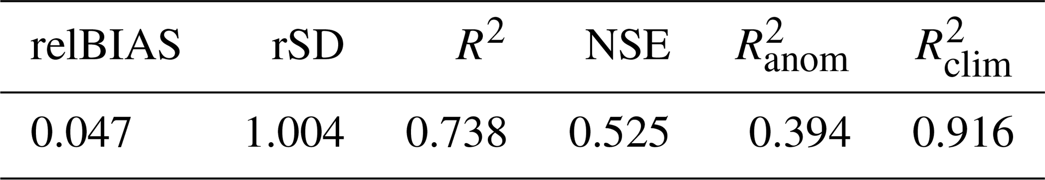
Figure 4 shows the spatial distribution of the considered skill scores based on the two cross-validation experiments CV-SREX and CV-SPACE, while Table 1 reports the median values of the grid-cell skill score distribution. The spatial patterns emerging from the two cross-validation experiments are very similar, with CV-SPACE displaying better scores because of the RFM ability to exploit local information to improve runoff estimates.
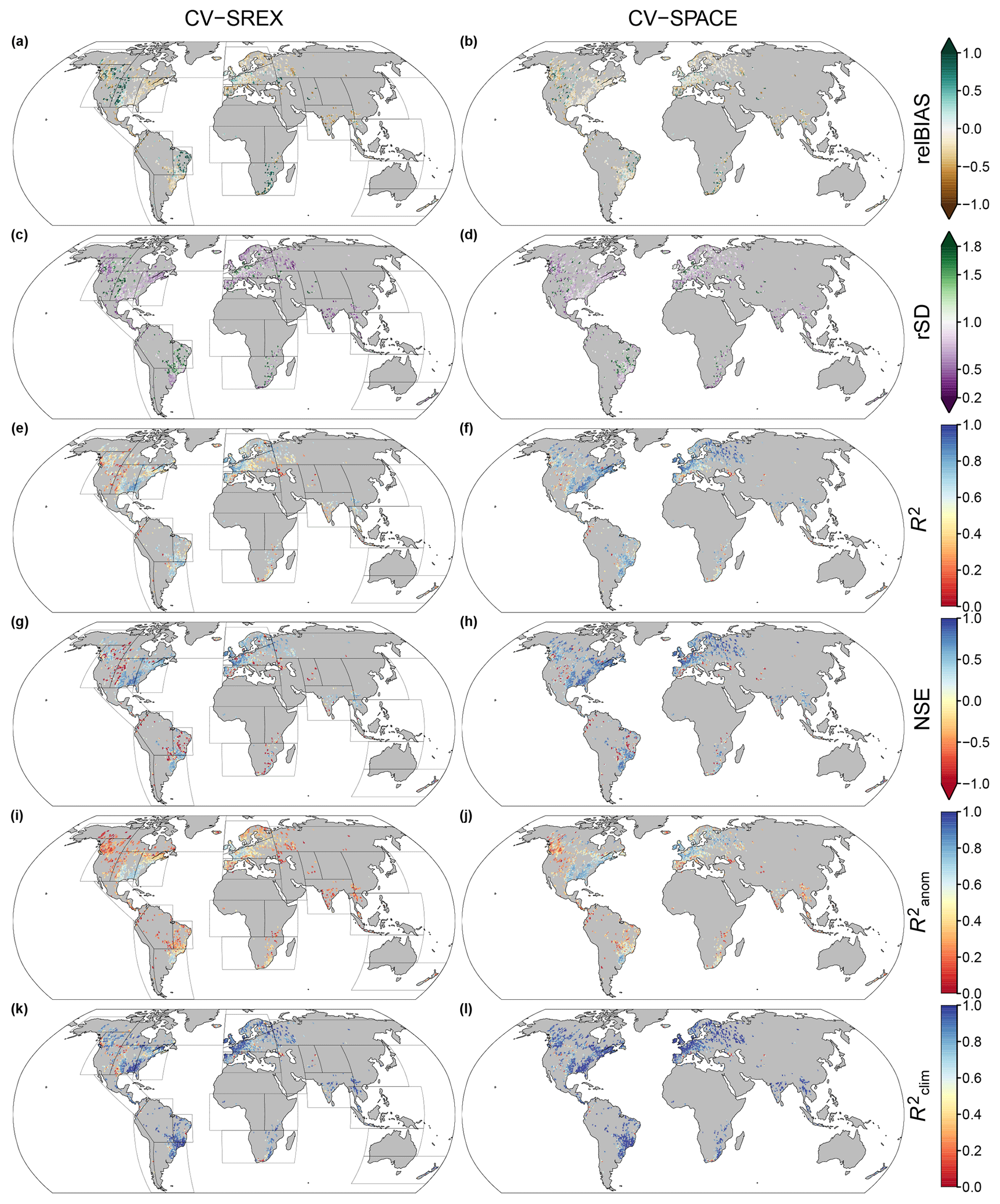
Figure 4Spatial distribution of the skill scores obtained from the CV-SREX (left) and CV-SPACE (right) experiments. SREX region boundaries are superimposed over the skill maps of CV-SREX.
Table 1Median values of skill scores for CV-SREX and CV-SPACE.

On average, the relBIAS of the RFM is slightly negative, indicating a tendency to underestimate monthly runoff rates (Fig. 4a–b). However, in arid regions such as the southwestern USA, northeastern Brazil and southern Africa, the RFM tends to overestimate the runoff (relBIAS is positive). Figure 4c–d show that when runoff is overestimated the variability tends to also be exaggerated (rSD is higher than 1). Oppositely, in the other areas, the variability is generally underestimated.
Overall, the runoff dynamics are well reproduced as indicated by high values of R2 (Fig. 4e–f). The NSE skill scores (Fig. 4g–h) show that in most regions of the world, RFM predictions are more skilful than the observed runoff long-term mean (NSE >0). The accuracy in reproducing runoff anomalies shows a more complex spatial pattern (Fig. 4i–j): humid regions and lowlands have quite high values, while decreasing skill is observed in mountainous regions and arid regions. Finally, Fig. 4k–l illustrate that the seasonal cycle of runoff is excellently reproduced across the whole globe. Figures S5 and S6 show the distribution of CV-SPACE skills of relBIAS, NSE and for each Köppen–Geiger (KG) climate zone (Peel et al., 2007) as well as the various SREX regions. The 25th, 50th and 75th quantiles of these skill distributions are reported in the “KG_CV_SPACE_Skills.csv” and “SREX_CV_SPACE_Skills.csv” files provided in the Supplement. Figures S7 and S8 show the cumulative distribution function of the monthly runoff rates and the monthly standardized anomalies for different climate zones respectively. In dry climates (group B of KG) we note an overestimation of GRUN in the lower part of the runoff rate distribution compared to the observation, although in terms of standardized anomalies the cumulative distribution of the estimate agrees very well with the observations.
5.2 Basin-scale validation
Figure 5a evaluates the accuracy of GRUN using the selected GRDC reference stations (Sect. 3.3), while Fig. 5b shows the observational agreement of river flow time series for some selected basins displayed in Fig. 5a. The temporal evolution of river flow is in general well captured and an underestimation of the peak flow volume is only evident for the Mekong River. For the Ebro the agreement between observations and GRUN starts to decrease from 1965 on. The dynamics are no longer well captured, and GRUN estimates are constantly higher than the GRDC observations. These discrepancies might be caused by the intensive irrigation and reservoir activities which have altered the natural hydrological regime of the basin. In that respect, it is interesting to notice that the NSE spatial pattern in Fig. 5a shows many similitudes with the estimated amount of runoff stored by engineered impoundments reported in Vörösmarty et al. (2004): low NSE scores tend to correspond to higher fractions of water impoundment. Both the Nile and Colorado river basins are exceptional examples of human-induced river flow alterations.
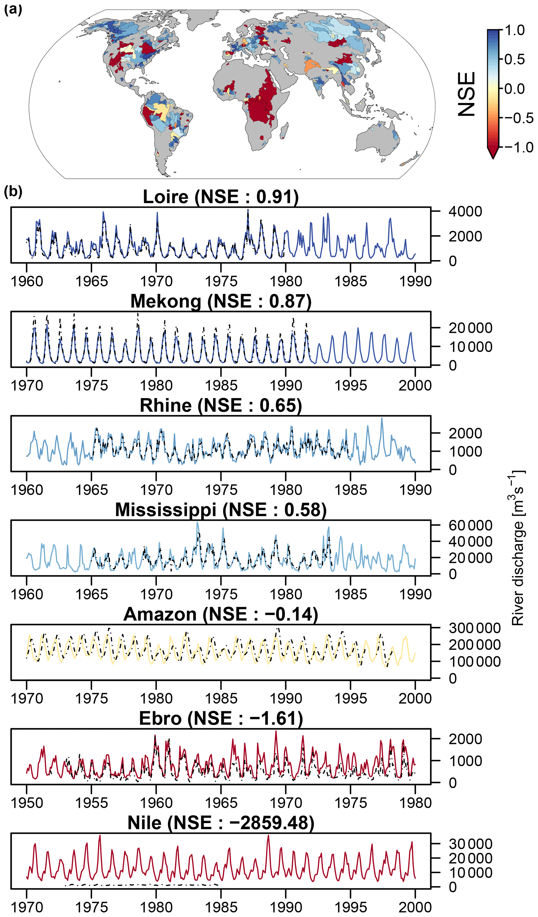
Figure 5Validation results based on selected GRDC river discharge observations. (a) Spatial distribution of the NSE skill for selected GRDC large basins. (b) Observed (dashed black line) and predicted (coloured) river discharge time series. Line colours correspond to the NSE skill shown in panel (a).
However, human activities are not the only cause of discrepancies between GRUN-based river discharge estimates and the observations. In the Amazon River, the negative NSE value and the visible phase lag between the estimated and the observed time series might not be caused by an inaccurate runoff reconstruction, but rather related to the fact that river discharge is simply estimated using the average runoff within the basin without taking water travel times into account. Indeed, for such an enormous river basin, a routing model accounting for water travel times would be necessary to correctly reproduce the river flow dynamics at monthly timescales. Figure S8 shows the spatial distribution of the remaining skill scores (e.g. other than NSE) for the GRDC basins.
5.3 Benchmarking against global hydrological models
In this section, we have benchmarked the performance of GRUN against well-established GHMs at two different scales.
Figure 6 compares the distribution of the skill scores for the CV-SREX and CV-SPACE experiments against the skill of the ISIMIP2a GHM runoff simulations of the nosoc experiment at the grid-cell scale. CV-SPACE always has higher skill than CV-SREX and outperforms all ISIMIP2a GHM runoff simulations and their multi-model ensemble mean (MMM) except for relBIAS and rSD. Overall, the GRUN cross-validation experiments show a tendency to underestimate runoff, although the skill spread of relBIAS is reduced compared to the ISIMIP2a models. Among the GHMs there is not a clear tendency to under- or overestimate runoff. The same applies for the variability (rSD). The dynamics of runoff (R2) are better reproduced by GRUN than by the considered GHMs, and the overall NSE skill score distribution is better for GRUN than for the ISIMIP2a GHM simulations. The anomalies () are also better reproduced by GRUN, and CV-SREX outperforms all the single GHMs. Finally, demonstrates that GRUN reproduces the seasonal cycle much better than the GHMs. Previous studies already showed that GHMs struggle in reproducing the seasonality of runoff (Gudmundsson et al., 2012; Gudmundsson and Seneviratne, 2015). Similar conclusions can be drawn by benchmarking GRUN against the pressoc and varsoc experiments of the ISIMIP2a runoff simulations (Figs. S2 and S3 respectively).
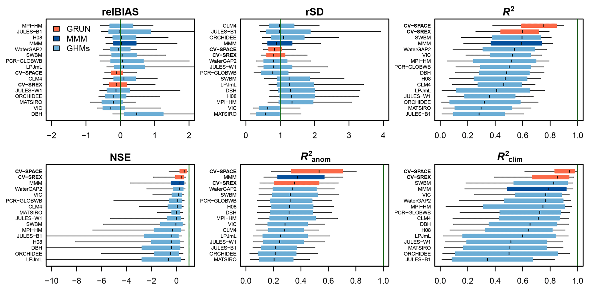
Figure 6Benchmarking the performance of GRUN against ISIMIP2a GHM runoff simulations (“nosoc” experiment). Box plot whiskers cover the 0.1 to 0.9 quantiles of the skill score distribution. The dark green vertical lines indicate the optimal score. GRUN cross-validation results are displayed in orange, while the multi-model mean (MMM) of ISIMIP2a GHM runoff simulations is displayed in dark blue. In most of the cases, the order of the boxes follows the rank of the median skill score. However, to avoid the compensatory effect with relBIAS and rSD scores, the individual boxes are ranked based on the absolute median value of the skill score minus the optimal score. The x axis of relBIAS is left and right truncated, for rSD it is right truncated and for NSE it is left truncated.
Because GHMs are typically not calibrated at the grid-cell scale (unlike GRUN), we have also benchmarked GRUN against ISIMIP2a GHM simulations in large river basins using the selection of GRDC reference stations with a catchment area larger than 10 000 km2 detailed in Sect. 3.3. The results for the ISIMIP2a nosoc, pressoc and varsoc scenarios are reported in Figs. S9, S10 and S11 respectively. The dynamics of runoff (R2), the anomalies and the climatology () are still better reproduced by GRUN than by the ISIMIP2a GHMs across all scenarios. The average relBIAS of GRUN is close to 0 while the variability is slightly overestimated: this contrasts the results obtained at the grid-cell scale where GRUN tends to underestimate the variability (rSD) compared to the observations. Figure S12 also provides a comparison of simulated river discharge from ISIMIP2a against 50 GRUN realizations (see Sect. 4.2) for the same time series displayed in Fig. 5, highlighting the larger scatter of conventional GHMs, likely due to structural and parameter uncertainties.
Table 2Median values of skill scores computed for the large GRDC river basins.
5.4 Sensitivity of the runoff estimates to the observations used for training
An ensemble of 50 runoff reconstructions trained on different subsets of observations (Sect. 4.2) is used to assess the sensitivity of GRUN to the observations used for training. Figure 7 shows the long-term mean of the monthly ensemble standard deviation and coefficient of variation (defined as the standard deviation divided by the mean). Regions characterized by higher runoff rates show higher standard deviation (Fig. 7a), but this variability across the realizations is small (<20 %) compared to the runoff magnitude (Fig. 7b). With the exception of arid regions, the coefficient of variation is generally below 0.2 (Fig. 7b).
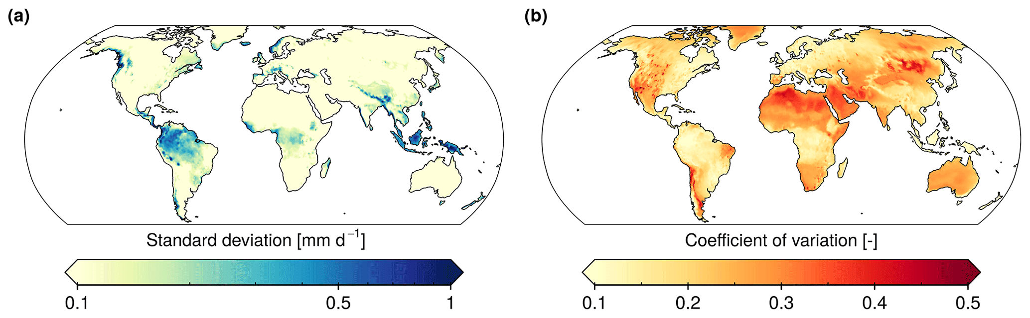
Figure 7Long-term mean of the monthly standard deviation of the runoff reconstruction ensemble (a) and the corresponding coefficient of variation (b).
To put the sensitivity of GRUN in relation to the observations used for training, Fig. 8 compares the annual runoff volumes of the GRUN realizations against the state-of-the-art GHMs participating in ISIMIP2a. The global long-term mean runoff volume estimated by GRUN (38 452 km3 yr−1) lies within the lower range of the ISIMIP2a GHMs (Fig. 8a) and generally agrees with other global terrestrial discharge estimates (Table 3). The uncertainty attributed to the selection of training observations (shaded area in Fig. 8a) of the global GRUN runoff volume is far smaller than the spread introduced by different physical representations of the hydrological processes in the GHMs. The uncertainty introduced by the selection of training observations increases proportionally to the magnitude of the runoff rates and is highest in the tropics (Fig. 8b). Reversely, the spread of the GHMs tends to be constant across all latitudes. GRUN almost always shows latitudinal mean runoff rates lower than the MMM and goes beyond the GHM range only between 20 and 30∘ latitude north. This pattern is mainly related to the relatively low runoff estimates in GRUN in northeastern India and Bangladesh compared to those of the GHMs (Fig. 8c).
Table 3Comparing global long-term mean runoff from GRUN against values reported in the literature. GRUN estimates are obtained by considering the same time span and spatial coverage of the reported studies. Values in parentheses denote the uncertainty range reported in some studies.
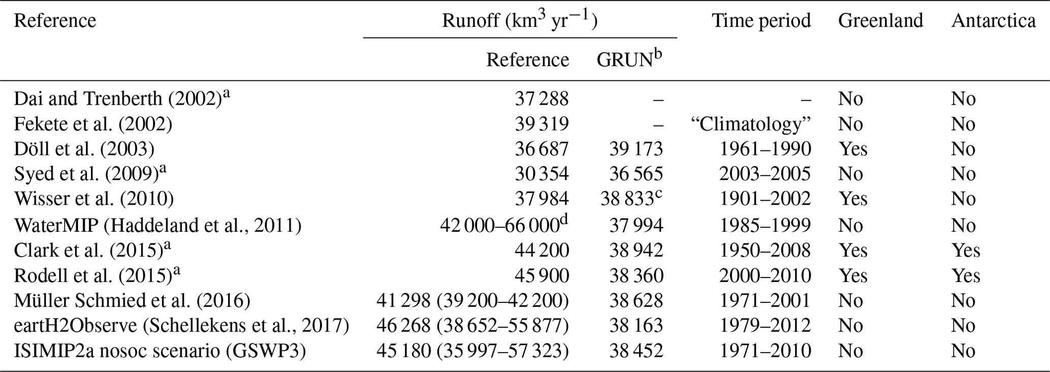
a The long-term mean is obtained by extrapolation from continental-scale river discharge observations or water balance. b Antarctica is never included in the GRUN estimate of the global long-term mean runoff. Greenland is considered only if included in the reference dataset. c GRUN long-term mean runoff is computed for the period 1902–2002. d Haddeland et al. (2011) report that the CRU land mask used to rescale global mean runoff (excluding Antarctica and Greenland) has an area of 1.44×10⁸ km2, while the correct area value should be around 1.33×10⁸ km2.
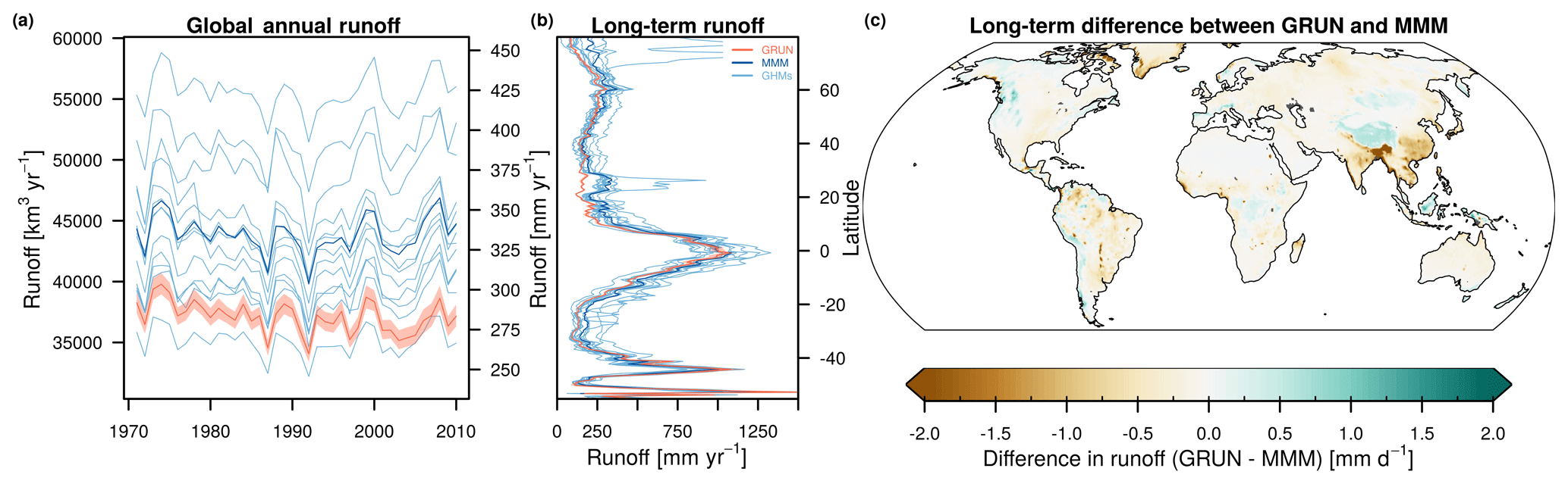
Figure 8The uncertainty of GRUN, attributed to the finite sample of training data, compared to the spread introduced by different physical representations of the hydrological processes in the ISIMIP2a GHMs. The shaded area around GRUN lines shows the entire distribution of the 50 GRUN simulations. (a) Global annual runoff. (b) Latitudinal average of long-term mean runoff. (c) Difference between GRUN and the MMM long-term mean runoff. Grey cells represent missing values caused by missing data in some of the ISIMIP2a GHM simulations.
5.5 Limitations of GRUN
The streamflow observations used for model training underwent careful preprocessing and screening steps to remove time series presenting sudden changes in the hydrological signature. Therefore, and because the product is solely forced with precipitation and temperature, GRUN is not able to explicitly account for the effects of local human river flow regulation (dam operations in particular) on the reconstructed hydrological regimes. However, we note that some streamflow observations impacted by irrigation or other land and water management practices have likely not been removed, especially if the magnitude of water abstraction/returns did not alter the monthly hydrograph sufficiently to identify a change point or if the time series is not long enough to cover past periods of near-natural streamflow. This may be one of the reasons for the overestimation of runoff rates in several arid regions (Fig. 4a–b) known for intensive-irrigation activities (Wriedt et al., 2009; Siebert et al., 2015). To some extent, the impact of past land-use changes on water availability might be implicitly accounted for in GRUN, for example if the GSWP3 bias-corrected reanalysis captured regional changes in precipitation and temperature induced by human activities (e.g. Davin et al., 2007; DeAngelis et al., 2010; Luyssaert et al., 2014; Alter et al., 2015; Thiery et al., 2017) or if water management practices are altered gradually together with a climate change signal (e.g. irrigation may increase with decreasing precipitation). Any changing pattern in water availability emerging from GRUN is however solely conditioned by trends of the GSWP3 forcing and the runoff observations used for model training. Thus, our evaluation is that GRUN estimates likely lie closer to near-natural runoff conditions than to human-regulated conditions (e.g. see the Nile River estimate in Fig. 5b), even though we cannot exclude that GRUN implicitly includes some human effects due to the various reasons mentioned above. Finally, we note that the accuracy of the runoff rates in mountainous regions is likely not optimal. The coarse resolution of the considered meteorological forcing does not allow capture of the sub-grid variability of precipitation and temperature that governs snowmelt volume and timing in such regions. Although the statistical model could implicitly account for homogenous biases in the forcing dataset and streamflow observations, the reader must be aware of possibly inconsistent water balance in such regions. Glacier melting is also not explicitly accounted for in GRUN.
6.1 Runoff climatology
Figure 9a displays the annual runoff climatology derived as the long-term mean of the GRUN reconstruction covering the 1902–2014 period. Long-term mean runoff rates differ by 3 orders of magnitude across the globe, with the highest rates in the tropics and large mountain ranges and lowest rates in the extratropics and major world deserts such as the Sahara. Monthly climatologies are provided in the Supplement (Fig. S13). Figure 9b and c show the months with the minimum and maximum of the mean seasonal runoff cycle. In the Northern Hemisphere, regions exposed to snow accumulation have the lowest runoff in winter and a runoff peak toward the end of spring as a result of snowpack melting and decreasing terrestrial water storage (Humphrey et al., 2016). In the humid mid-latitudes, evapotranspiration follows the seasonal cycle of temperature, causing the lowest (highest) runoff to occur prevalently during the summer (winter) months. In the tropics, maximum runoff tends to occur during the rainy season, which follows the migration of the Intertropical Convergence Zone (Schneider et al., 2014).
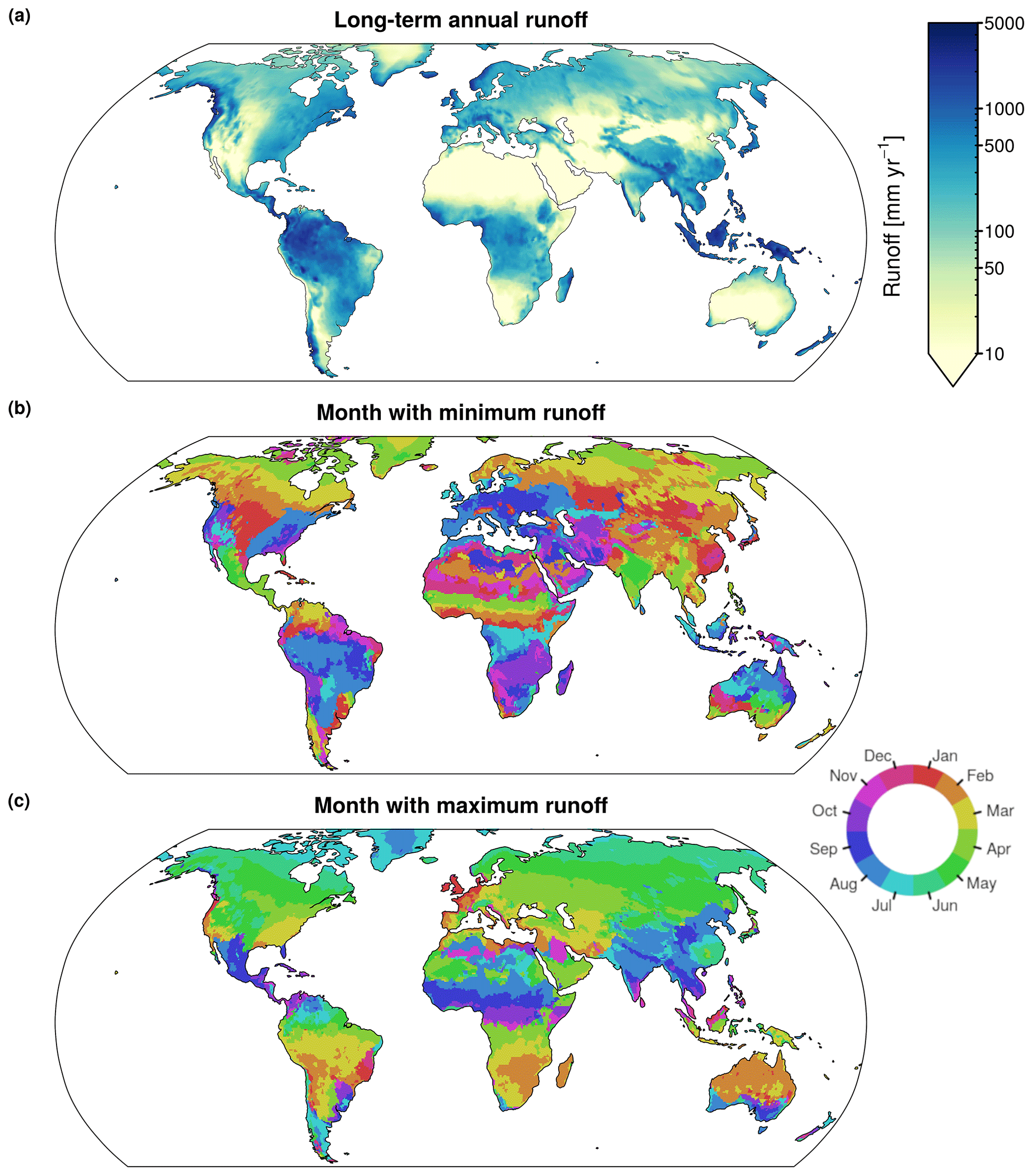
Figure 9Runoff climatology (1902–2014). (a) Long-term mean annual runoff rates. (b) Month with the minimum and (c) the maximum long-term mean monthly runoff.
6.2 Trends in reconstructed runoff
GRUN can be used to investigate changing freshwater availability. Trends in observed (Fig. 10a) and estimated (Fig. 10b) annual runoff for the period 1971–2010 are computed using Sen's slope (Sen, 1968) and expressed in absolute and relative terms. Overall, the reconstructed trends are in line with other reported findings (Gudmundsson et al., 2018a) and closely resemble the observed trends.
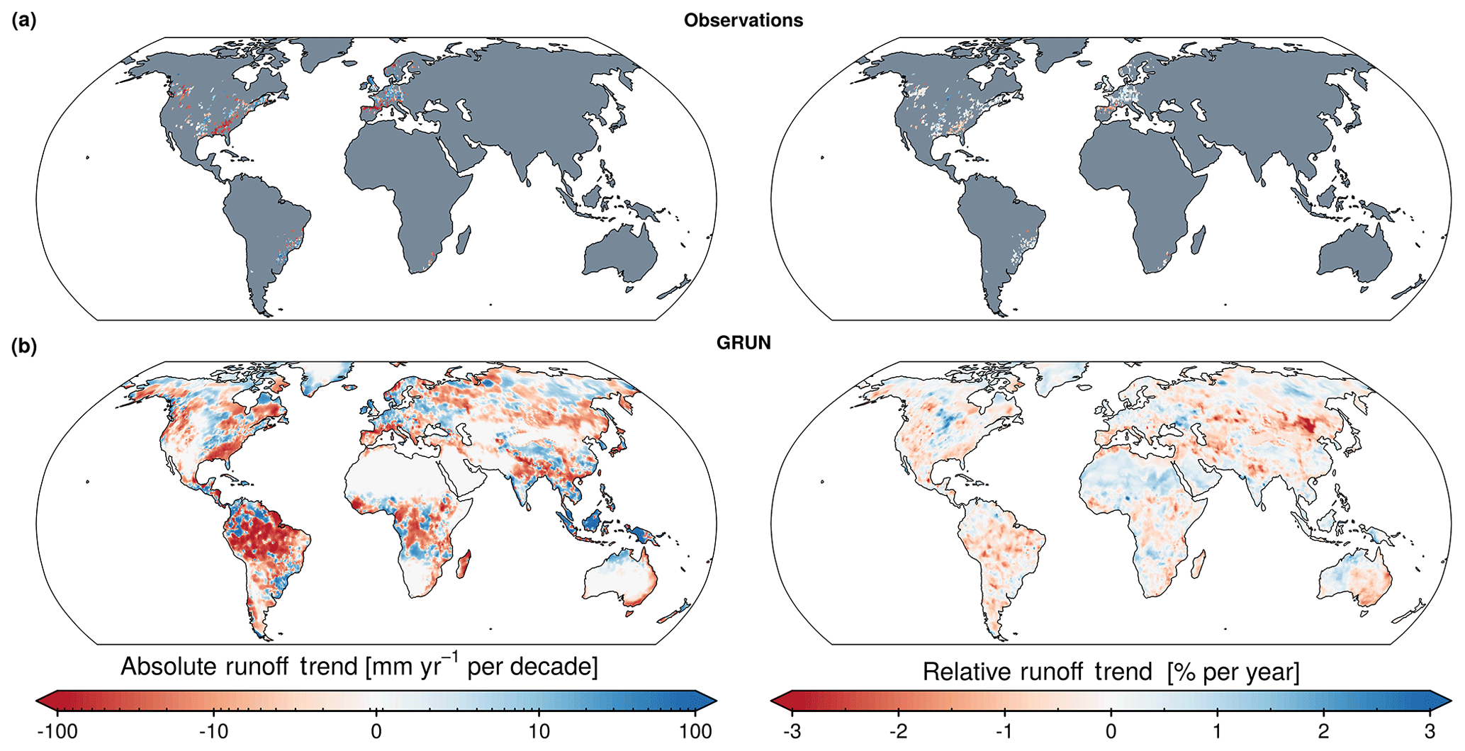
Figure 10Changes in annual runoff rates (1971–2010) expressed in absolute terms (left) and percentage change relative to long-term mean (right). (a) Observed trends. (b) Trends based on GRUN.
In Europe, the Mediterranean region exhibits a decrease in annual runoff, while in central and northern Europe there is a tendency towards increasing runoff rates. This pattern is in agreement with previous studies (Stahl et al., 2010, 2012) and was recently attributed to anthropogenic climate change (Gudmundsson et al., 2017). In the eastern and western USA negative trends occur, while large portions of the Mississippi River basin show increasing runoff.
In the tropics, the Amazon basin shows a substantial decrease in annual runoff rates. Studies have shown that a reduction of freshwater discharge to the Atlantic Ocean has the potential to impact the Atlantic and the Northern Hemisphere climate (Vizy and Cook, 2010; Jahfer et al., 2017). Considering the increasing human pressure to which this basin is currently exposed (Castello and Macedo, 2016; Latrubesse et al., 2017) and the uncertain impact of deforestation on river flow (D'Almeida et al., 2007; Spracklen et al., 2012; Lawrence and Vandecar, 2015; Spracklen and Garcia-Carreras, 2015), the causes and consequences of such trends should be investigated in more detail. Similarly, the drying tendency observed in many regions of the Congo Basin could affect the eastern equatorial Atlantic climate variability (Materia et al., 2012). Reversely, tropical areas in Southeast Asia experience an increase in runoff.
The monthly resolution of GRUN also allows investigation of these changes at sub-seasonal timescales (Fig. S14), which might be relevant for water resource assessments because neglecting the seasonal fluctuations can cause underestimation of water scarcity (Mekonnen and Hoekstra, 2016). In addition to changes in magnitude, the GSIM dataset also offers the possibility to analyse shifts in the seasonality of the hydrological regimes. Figure S15 provides an overview of the months in which the minimum and maximum runoff volumes occurred at the beginning and at the end of the 20th century. Over Europe for example, Fig. S15 shows evidence for earlier occurrence of maximum runoff, which is consistent with changes in snowmelt timing already reported in recent studies (Blöschl et al., 2017; Hall and Blöschl, 2018).
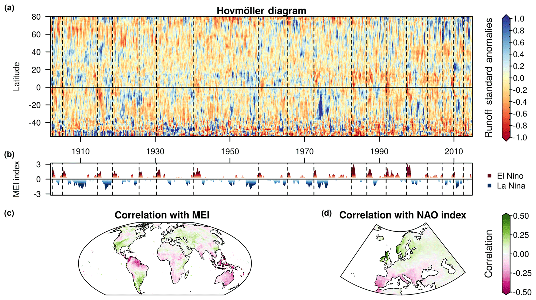
Figure 11Interannual variability of runoff and its relation to modes of climate variability. (a) Hovmöller diagram of standard runoff anomalies (reference period 1902–2014). Vertical dashed lines indicate onset of El Niño events. (b) Time series of the multivariate ENSO index (MEI). Red and blue shades characterize the intensity of El Niño and La Niña conditions respectively. (c) Correlation of the MEI with monthly runoff anomalies. (d) Relationship of European runoff anomalies with the North Atlantic Oscillation (NAO).
6.3 Interannual variability and teleconnections
The long temporal coverage of GRUN combined with its high skill in reproducing runoff dynamics provide an unprecedented opportunity to study the response of runoff to the modes of climate variability throughout the 20th and the early 21st centuries. The Hovmöller diagram in Fig. 11a illustrates the interannual runoff variability by showing the time evolution of the latitudinal mean of monthly runoff standard anomalies. The occurrence of El Niño events, defined here as the periods in which the multivariate El Niño–Southern Oscillation (ENSO) index (MEI) (Wolter and Timlin, 2011) is larger than 1, coincides with negative anomalies in the tropical regions. A correlation analysis between monthly standard anomalies of GRUN and the MEI time series reveals that during El Niño events, the Amazon basin, the Southeast Asia, Australia and southern Africa tend to experience lower runoff rates (Fig. 11c), which is consistent with previous assessments (Ward et al., 2010; Wanders and Wada, 2015). The opposite occurs during La Niña events, and drier conditions are observed in the western United States, which is also consistent with previous work (Tang et al., 2016).
As an additional example, Fig. 11d shows the influence of the North Atlantic Oscillation (NAO) on the European continent. The analysis confirms the previous finding that when NAO is positive, England and Scandinavia exhibit higher runoff rates, while southern Europe experiences drier conditions (Bouwer et al., 2006; Bierkens and van Beek, 2009; Lorenzo-Lacruz et al., 2011; Steirou et al., 2017).
6.4 Drought and agricultural productivity
GRUN can be used to study the spatio-temporal development of slowly evolving phenomena such as droughts. Since runoff can be defined as the excess of water available to ecosystems, negative runoff standard anomalies can be used as an indicator for droughts and potentially lower agricultural and vegetation productivity (GS15, GS16, Humphrey et al., 2018). Figure 12 shows three drought events that are known for their exceptional severity and devastating impact on agricultural production. Figure 12a displays the monthly runoff standard anomalies in August 1976 over Europe that according to our results ranks in the top five driest months (in terms of runoff anomaly) in large parts of England, northern France, central Europe and southern Sweden. Studies have shown that the drought mainly developed because of severe precipitation deficits (Zaidman et al., 2002; Spinoni et al., 2015) rather than extremely hot temperatures as it occurred during the 2015 drought (Ionita et al., 2017). Figure 12b reports the annual runoff standard anomalies in North America in the year 1934. This drought is known as the “Dust Bowl” and is unique for its spatial extent and duration. The negative runoff anomalies spanned the entire United States. Several studies have suggested that initial drying caused by La Niña conditions was amplified by human-induced land degradation of the US Great Plains (Schubert et al., 2004; Cook et al., 2009, 2014). During this event, dust storms severely damaged the American prairies by destroying millions of hectares of cultivated land. Finally, Fig. 12c illustrates the Horn of Africa drought conditions in 1984. The event also ranks in the most extreme events of the region and resulted in a widespread famine, which killed as many as 700 000 people in Ethiopia (Kidane, 1990). The drought was linked to El Niño conditions and a strong reduction in annual precipitation (Viste et al., 2013; Lanckriet et al., 2015).
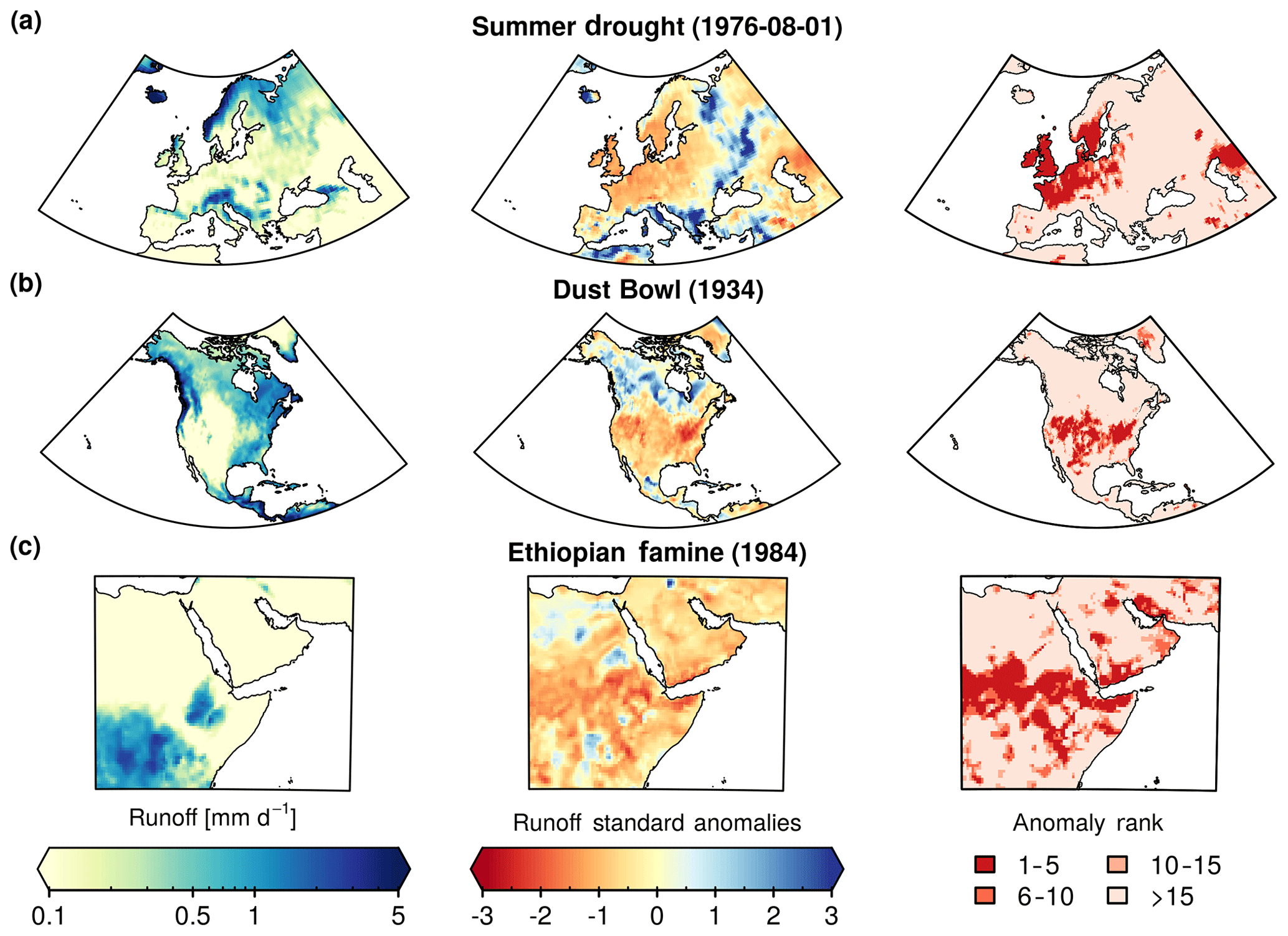
Figure 12Three extreme drought events as reconstructed by GRUN. (a) European summer drought in 1976. (b) US Dust Bowl in 1934. (c) Ethiopian famine in 1984.
The GRUN dataset based on GSWP3 forcing is publicly available in NetCDF-4 format (Ghiggi et al., 2019) and can be freely downloaded at https://doi.org/10.6084/m9.figshare.9228176.
This study presents an observationally driven global gridded reconstruction of monthly runoff rates derived using a machine learning algorithm. The dataset covers the period from 1902 to 2014 and is provided on a 0.5∘ × 0.5∘ WGS84 grid. The machine learning algorithm is trained with runoff observations from a global collection of in situ streamflow observations of relatively small catchments (<2500 km2) and uses gridded precipitation and temperature from a century-long reanalysis product as predictors. Model validation based on cross-validation experiments shows that the accuracy of the reconstruction is reasonable. On average GRUN shows higher predictive skills than a collection of state-of-the-art global hydrological models, especially with respect to the reproduction of the seasonality, dynamics and anomalies of runoff. At the monthly timescale, we find that a restricted number of predictors (i.e. precipitation and temperature) is sufficient to reproduce important aspects of terrestrial water dynamics. GRUN is thus an interesting candidate to evaluate and refine current parametrizations of global hydrological models as well as to potentially constrain fluxes of fine-resolution models (in space and time) through the adoption of multi-scale optimization techniques (Samaniego et al., 2010, 2017).
Since the GRUN reconstruction does not explicitly account for human flow regulation, differences between this reconstruction and in situ observations may help to identify heavily regulated locations on a global scale (Jaramillo and Destouni, 2015; Arheimer et al., 2017). GRUN offers a unique view of large-scale features of runoff variability in regions with limited or no observational coverage. The new dataset can be exploited (i) to study the onset and development of large-scale extreme events such as droughts, (ii) to investigate links between runoff and modes of climate variability, (iii) to conduct large-scale water resource assessments, (iv) to detect changes in water availability and dynamics, (v) to reconstruct droughts in the last millennium in combination with tree rings (Nicault et al., 2008; Cook et al., 2010a, b, 2015; Meko et al., 2012), (vi) to benchmark regional streamflow archives and hydrological reconstructions (Wang et al., 2009; Wu et al., 2011; Caillouet et al., 2017; Mishra et al., 2018; Moravec et al., 2019; Smith et al., 2019), and (vii) to address other scientific challenges in water cycle research (Wagener et al., 2010; Montanari et al., 2013; Greve et al., 2014; Trenberth and Asrar, 2014; Hegerl et al., 2015).
We conclude by remarking that this dataset would not have been possible without the mobilization of national and international hydrological archives. This study shows the benefit of a wider access to hydrological data collected by various institutions worldwide. We call for a continuation of the international efforts to reduce political and technical barriers for the exchange of hydrometeorological data across the scientific community.
The supplement related to this article is available online at: https://doi.org/10.5194/essd-11-1655-2019-supplement.
LG initiated this investigation. GG, VH, SIS and LG designed the study. GG developed the model code and performed the analysis. GG prepared the paper with contributions from all co-authors.
The authors declare that they have no conflict of interest.
We thank Hyungjun Kim for providing us with early access to the GSWP3 dataset and GRDC for the river discharge observations.
Sonia I. Seneviratne acknowledges partial support from the ERC DROUGHT-HEAT project funded by the European Community’s Seventh Framework Programme (grant agreement FP7-IDEAS-ERC-617518). Vincent Humphrey acknowledges support from the Swiss National Science Foundation (grant agreement P400P2_180784).
This paper was edited by Alexander Gelfan and reviewed by two anonymous referees.
Alter, R. E., Fan, Y., Lintner, B. R., and Weaver, C. P.: Observational Evidence that Great Plains Irrigation Has Enhanced Summer Precipitation Intensity and Totals in the Midwestern United States, J. Hydrometeorol., 16, 1717–1735, https://doi.org/10.1175/jhm-d-14-0115.1, 2015.
Arheimer, B., Donnelly, C., and Lindström, G.: Regulation of snow-fed rivers affects flow regimes more than climate change, Nat. Commun., 8, 62, https://doi.org/10.1038/s41467-017-00092-8, 2017.
Bierkens, M. F. P. and van Beek, L. P. H.: Seasonal Predictability of European Discharge: NAO and Hydrological Response Time, J. Hydrometeorol., 10, 953–968, https://doi.org/10.1175/2009JHM1034.1, 2009.
Blöschl, G., Sivapalan, M., Wagener, T., Viglione, A., and Savenije, H.: Runoff Prediction in Ungauged Basins: Synthesis Across Processes, Places and Scales, Cambridge University Press, 2013.
Blöschl, G., Hall, J., Parajka, J., Perdigão, R. A. P., Merz, B., Arheimer, B., Aronica, G. T., Bilibashi, A., Bonacci, O., Borga, M., Čanjevac, I., Castellarin, A., Chirico, G. B., Claps, P., Fiala, K., Frolova, N., Gorbachova, L., Gül, A., Hannaford, J., Harrigan, S., Kireeva, M., Kiss, A., Kjeldsen, T. R., Kohnová, S., Koskela, J. J., Ledvinka, O., Macdonald, N., Mavrova-Guirguinova, M., Mediero, L., Merz, R., Molnar, P., Montanari, A., Murphy, C., Osuch, M., Ovcharuk, V., Radevski, I., Rogger, M., Salinas, J. L., Sauquet, E., Šraj, M., Szolgay, J., Viglione, A., Volpi, E., Wilson, D., Zaimi, K., and Živković, N.: Changing climate shifts timing of European floods, Science, 357, 588–590, https://doi.org/10.1126/science.aan2506, 2017.
Bouwer, L. M., Vermaat, J. E., and Aerts, J. C. J. H.: Winter atmospheric circulation and river discharge in northwest Europe, Geophys. Res. Lett., 33, 2–5, https://doi.org/10.1029/2005GL025548, 2006.
Breiman, L.: Random forests, Mach. Learn., 45, 5–32, https://doi.org/10.1023/A:1010933404324, 2001.
Breiman, L., Friedman, J., Stone, C. J., and Olshen, R. A.: Classification and regression trees, Chapman and Hall, 1984.
Caillouet, L., Vidal, J.-P., Sauquet, E., Devers, A., and Graff, B.: Ensemble reconstruction of spatio-temporal extreme low-flow events in France since 1871, Hydrol. Earth Syst. Sci., 21, 2923–2951, https://doi.org/10.5194/hess-21-2923-2017, 2017.
Castello, L. and Macedo, M. N.: Large-scale degradation of Amazonian freshwater ecosystems, Glob. Change Biol., 22, 990–1007, https://doi.org/10.1111/gcb.13173, 2016.
Chen, J. and Gupta, A. K.: Parametric statistical change point analysis, Birkhäuser Boston, 2012.
Clark, E. A., Sheffield, J., van Vliet, M. T. H., Nijssen, B., and Lettenmaier, D. P.: Continental Runoff into the Oceans (1950–2008), J. Hydrometeorol., 16, 1502–1520, https://doi.org/10.1175/JHM-D-14-0183.1, 2015.
Compo, G. P., Whitaker, J. S., Sardeshmukh, P. D., Matsui, N., Allan, R. J., Yin, X., Gleason, B. E., Vose, R. S., Rutledge, G., Bessemoulin, P., BroNnimann, S., Brunet, M., Crouthamel, R. I., Grant, A. N., Groisman, P. Y., Jones, P. D., Kruk, M. C., Kruger, A. C., Marshall, G. J., Maugeri, M., Mok, H. Y., Nordli, O., Ross, T. F., Trigo, R. M., Wang, X. L., Woodruff, S. D., and Worley, S. J.: The Twentieth Century Reanalysis Project, Q. J. Roy. Meteor. Soc., 137, 1–28, https://doi.org/10.1002/qj.776, 2011.
Cook, B. I., Miller, R. L., and Seager, R.: Amplification of the North American “Dust Bowl” drought through human-induced land degradation, P. Natl. Acad. Sci. USA, 106, 4997–5001, https://doi.org/10.1073/pnas.0810200106, 2009.
Cook, B. I., Seager, R., and Smerdon, J. E.: The worst North American drought year of the last millennium: 1934, Geophys. Res. Lett., 41, 7298–7305, https://doi.org/10.1002/2014GL061661, 2014.
Cook, E. R., Anchukaitis, K. J., Jacoby, G. C., Wright, W. E., Buckley, B. M., and D'Arrigo, R. D.: Asian Monsoon Failure and Megadrought During the Last Millennium, Science, 328, 486–489, https://doi.org/10.1126/science.1185188, 2010a.
Cook, E. R., Seager, R., Heim, R. R., Vose, R. S., Herweijer, C., and Woodhouse, C.: Megadroughts in North America: Placing IPCC projections of hydroclimatic change in a long-term palaeoclimate context, J. Quaternary Sci., 25, 48–61, https://doi.org/10.1002/jqs.1303, 2010b.
Cook, E. R., Seager, R., Kushnir, Y., Briffa, K. R., Büntgen, U., Frank, D., Krusic, P. J., Tegel, W., van der Schrier, G., Andreu-Hayles, L., Baillie, M., Baittinger, C., Bleicher, N., Bonde, N., Brown, D., Carrer, M., Cooper, R., Čufar, K., Dittmar, C., Esper, J., Griggs, C., Gunnarson, B., Günther, B., Gutierrez, E., Haneca, K., Helama, S., Herzig, F., Heussner, K.-U., Hofmann, J., Janda, P., Kontic, R., Köse, N., Kyncl, T., Levanič, T., Linderholm, H., Manning, S., Melvin, T. M., Miles, D., Neuwirth, B., Nicolussi, K., Nola, P., Panayotov, M., Popa, I., Rothe, A., Seftigen, K., Seim, A., Svarva, H., Svoboda, M., Thun, T., Timonen, M., Touchan, R., Trotsiuk, V., Trouet, V., Walder, F., Wazny, T., Wilson, R., and Zang, C.: Old World megadroughts and pluvials during the Common Era, Sci. Adv., 1, e1500561, https://doi.org/10.1126/sciadv.1500561, 2015.
Dai, A. and Trenberth, K. E.: Estimates of Freshwater Discharge from Continents: Latitudinal and Seasonal Variations, J. Hydrometeorol., 3, 660–687, https://doi.org/10.1175/1525-7541(2002)003<0660:EOFDFC>2.0.CO;2, 2002.
D'Almeida, C., Vörösmarty, C. J., Hurtt, G. C., Marengo, J. A., Dingman, S. L., and Keim, B. D.: The effects of deforestation on the hydrological cycle in Amazonia: A review on scale and resolution, Int. J. Climatol., 27, 633–647, https://doi.org/10.1002/joc.1475, 2007.
Davin, E. L., de Noblet-Ducoudré, N., and Friedlingstein, P.: Impact of land cover change on surface climate: Relevance of the radiative forcing concept, Geophys. Res. Lett., 34, 1–5, https://doi.org/10.1029/2007GL029678, 2007.
DeAngelis, A., Dominguez, F., Fan, Y., Robock, A., Kustu, M. D., and Robinson, D.: Evidence of enhanced precipitation due to irrigation over the Great Plains of the United States, J. Geophys. Res.-Atmos., 115, 1–14, https://doi.org/10.1029/2010JD013892, 2010.
Dirmeyer, P. A.: A History and Review of the Global Soil Wetness Project (GSWP), J. Hydrometeorol., 12, 729–749, https://doi.org/10.1175/JHM-D-10-05010.1, 2011.
Dirmeyer, P. A., Gao, X., Zhao, M., Guo, Z., Oki, T., and Hanasaki, N.: GSWP-2: Multimodel analysis and implications for our perception of the land surface, B. Am. Meteorol. Soc., 87, 1381–1397, https://doi.org/10.1175/BAMS-87-10-1381, 2006.
Do, H. X., Gudmundsson, L., Leonard, M., and Westra, S.: The Global Streamflow Indices and Metadata Archive (GSIM) – Part 1: The production of a daily streamflow archive and metadata, Earth Syst. Sci. Data, 10, 765–785, https://doi.org/10.5194/essd-10-765-2018, 2018.
Döll, P., Kaspar, F., and Lehner, B.: A global hydrological model for deriving water availability indicators: Model tuning and validation, J. Hydrol., 270, 105–134, https://doi.org/10.1016/S0022-1694(02)00283-4, 2003.
Fekete, B. M. and Vörösmarty, C. J.: The current status of global river discharge monitoring and potential new technologies complementing traditional discharge measurements, IAHS Publ., 309, 129–136, 2007.
Fekete, B. M., Vörösmarty, C. J., and Grabs, W.: High-resolution fields of global runoff combining observed river discharge and simulated water balances, Global Biogeochem. Cy., 16, 15–1–15–10, https://doi.org/10.1029/1999GB001254, 2002.
Fekete, B. M., Looser, U., Pietroniro, A., and Robarts, R. D.: Rationale for Monitoring Discharge on the Ground, J. Hydrometeorol., 13, 1977–1986, https://doi.org/10.1175/JHM-D-11-0126.1, 2012.
Fekete, B. M., Robarts, R. D., Kumagai, M., Nachtnebel, H. P., Odada, E., and Zhulidov, A. V.: Time for in situ renaissance, Science, 349, 685–686, https://doi.org/10.1126/science.aac7358, 2015.
Ghiggi, G.: Reconstruction of European monthly runoff and river flow from 1951 to 2015 using machine learning algorithms, Master Thesis, ETHZ, 2018.
Ghiggi, G., Seneviratne, S. I., Humphrey, V., and Gudmundsson, L.: GRUN: Global Runoff Reconstruction, figshare, https://doi.org/10.6084/m9.figshare.9228176, 2019.
Gosling, S. N., Müller Schmied, H., Betts, R., Chang, J., Ciais, P., Dankers, R., Döll, P., Eisner, S., Flörke, M., Gerten, D., Grillakis, M., Hanasaki, N., Hagemann, S., Huang, M., Huang, Z., Jerez, S., Kim, H., Koutroulis, A., Leng, G., Liu, X., Masaki, Y., Montavez, P., Morfopoulos, C., Oki, T., Papadimitriou, L., Pokhrel, Y., Portmann, F. T., Orth, R., Ostberg, S., Satoh, Y., Seneviratne, S., Sommer, P., Stacke, T., Tang, Q., Tsanis, I., Wada, Y., Zhou, T., Büchner, M., Schewe, J., and Zhao, F.: ISIMIP2a Simulation Data from Water (global) Sector, GFZ Data Serv., https://doi.org/10.5880/PIK.2017.010, 2017.
Greve, P., Orlowsky, B., Mueller, B., Sheffield, J., Reichstein, M., and Seneviratne, S. I.: Global assessment of trends in wetting and drying over land, Nat. Geosci., 7, 716–721, https://doi.org/10.1038/NGEO2247, 2014.
Gudmundsson, L. and Seneviratne, S. I.: Towards observation-based gridded runoff estimates for Europe, Hydrol. Earth Syst. Sci., 19, 2859–2879, https://doi.org/10.5194/hess-19-2859-2015, 2015.
Gudmundsson, L. and Seneviratne, S. I.: Observation-based gridded runoff estimates for Europe (E-RUN version 1.1), Earth Syst. Sci. Data, 8, 279–295, https://doi.org/10.5194/essd-8-279-2016, 2016.
Gudmundsson, L., Tallaksen, L. M., Stahl, K., Clark, D. B., Dumont, E., Hagemann, S., Bertrand, N., Gerten, D., Heinke, J., Hanasaki, N., Voss, F., and Koirala, S.: Comparing Large-Scale Hydrological Model Simulations to Observed Runoff Percentiles in Europe, J. Hydrometeorol., 13, 604–620, https://doi.org/10.1175/JHM-D-11-083.1, 2012.
Gudmundsson, L., Seneviratne, S. I., and Zhang, X.: Anthropogenic climate change detected in European renewable freshwater resources, Nat. Clim. Change, 7, 813–816, https://doi.org/10.1038/nclimate3416, 2017.
Gudmundsson, L., Leonard, M., Do, H. X., Westra, S., and Seneviratne, S. I.: Observed Trends in Global Indicators of Mean and Extreme Streamflow, Geophys. Res. Lett., 46, 756–766, https://doi.org/10.1029/2018GL079725, 2018a.
Gudmundsson, L., Do, H. X., Leonard, M., and Westra, S.: The Global Streamflow Indices and Metadata Archive (GSIM) – Part 2: Quality control, time-series indices and homogeneity assessment, Earth Syst. Sci. Data, 10, 787–804, https://doi.org/10.5194/essd-10-787-2018, 2018b.
Haddeland, I., Clark, D. B., Franssen, W., Ludwig, F., Vöss, F., Arnell, N. W., Bertrand, N., Best, M., Folwell, S., Gerten, D., Gomes, S., Gosling, S. N., Hagemann, S., Hanasaki, N., Harding, R., Heinke, J., Kabat, P., Koirala, S., Oki, T., Polcher, J., Stacke, T., Viterbo, P., Weedon, G. P., and Yeh, P.: Multimodel Estimate of the Global Terrestrial Water Balance: Setup and First Results, J. Hydrometeorol., 12, 869–884, https://doi.org/10.1175/2011JHM1324.1, 2011.
Hall, J. and Blöschl, G.: Spatial patterns and characteristics of flood seasonality in Europe, Hydrol. Earth Syst. Sci., 22, 3883–3901, https://doi.org/10.5194/hess-22-3883-2018, 2018.
Harding, R., Best, M., Blyth, E., Hagemann, S., Kabat, P., Tallaksen, L. M., Warnaars, T., Wiberg, D., Weedon, G. P., van Lanen, H., Ludwig, F., and Haddeland, I.: WATCH: Current Knowledge of the Terrestrial Global Water Cycle, J. Hydrometeorol., 12, 1149–1156, https://doi.org/10.1175/JHM-D-11-024.1, 2011.
Hastie, T., Tibsharani, R., and Friedman, J. H.: The Elements of Statistical Learning, 2nd Edn., Springer, New York, 2009.
Hegerl, G. C., Black, E., Allan, R. P., Ingram, W. J., Polson, D., Trenberth, K. E., Chadwick, R. S., Arkin, P. A., Sarojini, B. B., Becker, A., Dai, A., Durack, P. J., Easterling, D., Fowler, H. J., Kendon, E. J., Huffman, G. J., Liu, C., Marsh, R., New, M., Osborn, T. J., Skliris, N., Stott, P. A., Vidale, P.-L., Wijffels, S. E., Wilcox, L. J., Willett, K. M., and Zhang, X.: Challenges in Quantifying Changes in the Global Water Cycle, B. Am. Meteorol. Soc., 96, 1097–1115, https://doi.org/10.1175/BAMS-D-13-00212.1, 2015.
Hrachowitz, M., Savenije, H. H. G., Blöschl, G., McDonnell, J. J., Sivapalan, M., Pomeroy, J. W., Arheimer, B., Blume, T., Clark, M. P., Ehret, U., Fenicia, F., Freer, J. E., Gelfan, A., Gupta, H. V., Hughes, D. A., Hut, R. W., Montanari, A., Pande, S., Tetzlaff, D., Troch, P. A., Uhlenbrook, S., Wagener, T., Winsemius, H. C., Woods, R. A., Zehe, E., and Cudennec, C.: A decade of Predictions in Ungauged Basins (PUB) – a review, Hydrolog. Sci. J., 58, 1198–1255, https://doi.org/10.1080/02626667.2013.803183, 2013.
Humphrey, V., Gudmundsson, L., and Seneviratne, S. I.: Assessing Global Water Storage Variability from GRACE: Trends, Seasonal Cycle, Subseasonal Anomalies and Extremes, Surv. Geophys., 37, 357–395, https://doi.org/10.1007/s10712-016-9367-1, 2016.
Humphrey, V., Zscheischler, J., Ciais, P., Gudmundsson, L., Sitch, S., and Seneviratne, S. I.: Sensitivity of atmospheric CO2 growth rate to observed changes in terrestrial water storage, Nature, 560, 628–631, https://doi.org/10.1038/s41586-018-0424-4, 2018.
Ionita, M., Tallaksen, L. M., Kingston, D. G., Stagge, J. H., Laaha, G., Van Lanen, H. A. J., Scholz, P., Chelcea, S. M., and Haslinger, K.: The European 2015 drought from a climatological perspective, Hydrol. Earth Syst. Sci., 21, 1397–1419, https://doi.org/10.5194/hess-21-1397-2017, 2017.
Jahfer, S., Vinayachandran, P. N., and Nanjundiah, R. S.: Long-Term impact of Amazon river runoff on northern hemispheric climate, Nat. Sci. Rep., 7, 10989, https://doi.org/10.1038/s41598-017-10750-y, 2017.
Jaramillo, F. and Destouni, G.: Local flow regulation and irrigation raise global human water consumption and footprint, Science, 350, 1248–1251, https://doi.org/10.1126/science.aad1010, 2015.
Kidane, A.: Mortality estimates of the 1984-85 Ethiopian famine, Scand. J. Soc. Med., 18, 281–286, https://doi.org/10.1177/140349489001800409, 1990.
Kim, H., Watanabe, S., Chang, E. C., Yoshimura, K., Hirabayashi, J., Famiglietti, J., and Oki, T.: Global Soil Wetness Project Phase 3 Atmospheric Boundary Conditions (Experiment 1) [Data set], Data Integration and Analysis System (DIAS), https://doi.org/10.20783/DIAS.501, 2017.
Kummu, M., Guillaume, J. H. A., de Moel, H., Eisner, S., Flörke, M., Porkka, M., Siebert, S., Veldkamp, T. I. E., and Ward, P. J.: The world's road to water scarcity: shortage and stress in the 20th century and pathways towards sustainability, Nat. Sci. Rep., 6, 38495, https://doi.org/10.1038/srep38495, 2016.
Lanckriet, S., Frankl, A., Adgo, E., Termonia, P., and Nyssen, J.: Droughts related to quasi-global oscillations: A diagnostic teleconnection analysis in North Ethiopia, Int. J. Climatol., 35, 1534–1542, https://doi.org/10.1002/joc.4074, 2015.
Latrubesse, E. M., Arima, E. Y., Dunne, T., Park, E., Baker, V. R., D'Horta, F. M., Wight, C., Wittmann, F., Zuanon, J., Baker, P. A., Ribas, C. C., Norgaard, R. B., Filizola, N., Ansar, A., Flyvbjerg, B., and Stevaux, J. C.: Damming the rivers of the Amazon basin, Nature, 546, 363–369, https://doi.org/10.1038/nature22333, 2017.
Laudon, H., Spence, C., Buttle, J., Carey, S. K., McDonnell, J. J., McNamara, J. P., Soulsby, C., and Tetzlaff, D.: Save northern high-latitude catchments, Nat. Geosci., 10, 324–325, https://doi.org/10.1038/ngeo2947, 2017.
Lawrence, D. and Vandecar, K.: Effects of tropical deforestation on climate and agriculture, Nat. Clim. Change, 5, 27–36, https://doi.org/10.1038/nclimate2430, 2015.
Lorenzo-Lacruz, J., Vicente-Serrano, S. M., López-Moreno, J. I., González-Hidalgo, J. C., and Morán-Tejeda, E.: The response of Iberian rivers to the North Atlantic Oscillation, Hydrol. Earth Syst. Sci., 15, 2581–2597, https://doi.org/10.5194/hess-15-2581-2011, 2011.
Luyssaert, S., Jammet, M., Stoy, P. C., Estel, S., Pongratz, J., Ceschia, E., Churkina, G., Don, A., Erb, K., Ferlicoq, M., Gielen, B., Grünwald, T., Houghton, R. A., Klumpp, K., Knohl, A., Kolb, T., Kuemmerle, T., Laurila, T., Lohila, A., Loustau, D., McGrath, M. J., Meyfroidt, P., Moors, E. J., Naudts, K., Novick, K., Otto, J., Pilegaard, K., Pio, C. A., Rambal, S., Rebmann, C., Ryder, J., Suyker, A. E., Varlagin, A., Wattenbach, M., and Dolman, A. J.: Land management and land-cover change have impacts of similar magnitude on surface temperature, Nat. Clim. Change, 4, 389–393, https://doi.org/10.1038/nclimate2196, 2014.
Materia, S., Gualdi, S., Navarra, A., and Terray, L.: The effect of Congo River freshwater discharge on Eastern Equatorial Atlantic climate variability, Clim. Dynam., 39, 2109–2125, https://doi.org/10.1007/s00382-012-1514-x, 2012.
Meko, D. M., Woodhouse, C. A., and Morino, K.: Dendrochronology and links to streamflow, J. Hydrol., 412–413, 200–209, https://doi.org/10.1016/j.jhydrol.2010.11.041, 2012.
Mekonnen, M. and Hoekstra, Y. A.: Four Billion People Experience Water Scarcity, Sci. Adv., 2, 1–7, https://doi.org/10.1126/sciadv.1500323, 2016.
Meyer, H., Reudenbach, C., Hengl, T., Katurji, M., and Nauss, T.: Improving performance of spatio-temporal machine learning models using forward feature selection and target-oriented validation, Environ. Model. Softw., 101, 1–9, https://doi.org/10.1016/j.envsoft.2017.12.001, 2018.
Mishra, V., Shah, R., Azhar, S., Shah, H., Modi, P., and Kumar, R.: Reconstruction of droughts in India using multiple land-surface models (1951–2015), Hydrol. Earth Syst. Sci., 22, 2269–2284, https://doi.org/10.5194/hess-22-2269-2018, 2018.
Montanari, A., Young, G., Savenije, H. H. G., Hughes, D., Wagener, T., Ren, L. L., Koutsoyiannis, D., Cudennec, C., Toth, E., Grimaldi, S., Blöschl, G., Sivapalan, M., Beven, K., Gupta, H., Hipsey, M., Schaefli, B., Arheimer, B., Boegh, E., Schymanski, S. J., Di Baldassarre, G., Yu, B., Hubert, P., Huang, Y., Schumann, A., Post, D. A., Srinivasan, V., Harman, C., Thompson, S., Rogger, M., Viglione, A., McMillan, H., Characklis, G., Pang, Z., and Belyaev, V.: “Panta Rhei-Everything Flows”: Change in hydrology and society-The IAHS Scientific Decade 2013–2022, Hydrolog. Sci. J., 58, 1256–1275, https://doi.org/10.1080/02626667.2013.809088, 2013.
Moravec, V., Markonis, Y., Rakovec, O., Kumar, R., and Hanel, M.: A 250-year European drought inventory derived from ensemble hydrologic modelling, Geophys. Res. Lett., 46, 5909–5917, https://doi.org/10.1029/2019gl082783, 2019.
Müller Schmied, H., Adam, L., Eisner, S., Fink, G., Flörke, M., Kim, H., Oki, T., Portmann, F. T., Reinecke, R., Riedel, C., Song, Q., Zhang, J., and Döll, P.: Variations of global and continental water balance components as impacted by climate forcing uncertainty and human water use, Hydrol. Earth Syst. Sci., 20, 2877–2898, https://doi.org/10.5194/hess-20-2877-2016, 2016.
Munia, H. A., Guillaume, J. H. A., Mirumachi, N., Wada, Y., and Kummu, M.: How downstream sub-basins depend on upstream inflows to avoid scarcity: typology and global analysis of transboundary rivers, Hydrol. Earth Syst. Sci., 22, 2795–2809, https://doi.org/10.5194/hess-22-2795-2018, 2018.
Nash, J. E. and Sutcliffe, J. V.: River flow forecasting through conceptual models part I – A discussion of principles, J. Hydrol., 10, 282–290, https://doi.org/10.1016/0022-1694(70)90255-6, 1970.
Nicault, A., Alleaume, S., Brewer, S., Carrer, M., Nola, P., and Guiot, J.: Mediterranean drought fluctuation during the last 500 years based on tree-ring data, Clim. Dynam., 31, 227–245, https://doi.org/10.1007/s00382-007-0349-3, 2008.
Oki, T. and Kanae, S.: Global Hydrological Cycles and Word Water Resources, Science, 313, 1068–1072, https://doi.org/10.1126/science.1128845, 2006.
Peel, M. C., Finlayson, B. L., and McMahon, T. A.: Updated world map of the Köppen-Geiger climate classification, Hydrol. Earth Syst. Sci., 11, 1633–1644, https://doi.org/10.5194/hess-11-1633-2007, 2007.
Rodell, M., Beaudoing, H. K., L'Ecuyer, T. S., Olson, W. S., Famiglietti, J. S., Houser, P. R., Adler, R., Bosilovich, M. G., Clayson, C. A., Chambers, D., Clark, E., Fetzer, E. J., Gao, X., Gu, G., Hilburn, K., Huffman, G. J., Lettenmaier, D. P., Liu, W. T., Robertson, F. R., Schlosser, C. A., Sheffield, J., and Wood, E. F.: The observed state of the water cycle in the early twenty-first century, J. Climate, 28, 8289–8318, https://doi.org/10.1175/JCLI-D-14-00555.1, 2015.
Samaniego, L., Kumar, R., and Attinger, S.: Multiscale parameter regionalization of a grid-based hydrologic model at the mesoscale, Water Resour. Res., 46, W05523, https://doi.org/10.1029/2008WR007327, 2010.
Samaniego, L., Kumar, R., Thober, S., Rakovec, O., Zink, M., Wanders, N., Eisner, S., Müller Schmied, H., Sutanudjaja, E. H., Warrach-Sagi, K., and Attinger, S.: Toward seamless hydrologic predictions across spatial scales, Hydrol. Earth Syst. Sci., 21, 4323–4346, https://doi.org/10.5194/hess-21-4323-2017, 2017.
Schellekens, J., Dutra, E., Martínez-de la Torre, A., Balsamo, G., van Dijk, A., Sperna Weiland, F., Minvielle, M., Calvet, J.-C., Decharme, B., Eisner, S., Fink, G., Flörke, M., Peßenteiner, S., van Beek, R., Polcher, J., Beck, H., Orth, R., Calton, B., Burke, S., Dorigo, W., and Weedon, G. P.: A global water resources ensemble of hydrological models: the eartH2Observe Tier-1 dataset, Earth Syst. Sci. Data, 9, 389–413, https://doi.org/10.5194/essd-9-389-2017, 2017.
Schneider, T., Bischoff, T., and Haug, G. H.: Migrations and dynamics of the intertropical convergence zone, Nature, 513, 45–53, https://doi.org/10.1038/nature13636, 2014.
Schubert, S. D., Suarez, M. J., Pegion, P. J., Koster, R. D., and Bacmeister, T.: On the Cause of the 1930s Dust Bowl, Science, 303, 1855–1859, https://doi.org/10.1126/science.1095048, 2004.
Sen, P. K.: Estimates of the Regression Coefficient Based on Kendall's Tau, J. Am. Stat. Assoc., 63, 1379–1389, https://doi.org/10.1080/01621459.1968.10480934, 1968.
Seneviratne, S. I., Nicholls, N., Easterling, D., Goodess, C. M., Kanae, S., Kossin, J., Luo, Y., Marengo, J., Mc Innes, K., Rahimi, M., Reichstein, M., Sorteberg, A., Vera, C., Zhang, X., Rusticucci, M., Semenov, V., Alexander, L. V., Allen, S., Benito, G., Cavazos, T., Clague, J., Conway, D., Della-Marta, P. M., Gerber, M., Gong, S., Goswami, B. N., Hemer, M., Huggel, C., Van den Hurk, B., Kharin, V. V., Kitoh, A., Klein Tank, A. M. G., Li, G., Mason, S., Mc Guire, W., Van Oldenborgh, G. J., Orlowsky, B., Smith, S., Thiaw, W., Velegrakis, A., Yiou, P., Zhang, T., Zhou, T., and Zwiers, F. W.: Changes in climate extremes and their impacts on the natural physical environment, in Managing the Risks of Extreme Events and Disasters to Advance Climate Change Adaptation: Special Report of the Intergovernmental Panel on Climate Change, Cambridge University Press, 109–230, 2012.
Shiklomanov, A. I., Lammers, R. B., and Vörösmarty, C. J.: Widespread decline in hydrological monitoring threatens Pan-Arctic research, Eos, 83, 13–17, https://doi.org/10.1029/2002EO000007, 2002.
Siebert, S., Kummu, M., Porkka, M., Döll, P., Ramankutty, N., and Scanlon, B. R.: A global data set of the extent of irrigated land from 1900 to 2005, Hydrol. Earth Syst. Sci., 19, 1521–1545, https://doi.org/10.5194/hess-19-1521-2015, 2015.
Sivapalan, M.: Prediction in ungauged basins: a grand challenge for theoretical hydrology, Hydrol. Process., 17, 3163–3170, https://doi.org/10.1002/hyp.5155, 2003.
Smith, K. A., Barker, L. J., Tanguy, M., Parry, S., Harrigan, S., Legg, T. P., Prudhomme, C., and Hannaford, J.: A multi-objective ensemble approach to hydrological modelling in the UK: an application to historic drought reconstruction, Hydrol. Earth Syst. Sci., 23, 3247–3268, https://doi.org/10.5194/hess-23-3247-2019, 2019.
Spinoni, J., Naumann, G., Vogt, J. V., and Barbosa, P.: The biggest drought events in Europe from 1950 to 2012, J. Hydrol. Reg. Stud., 3, 509–524, https://doi.org/10.1016/j.ejrh.2015.01.001, 2015.
Spracklen, D. V. and Garcia-Carreras, L.: The impact of Amazonian deforestation on Amazon basin rainfall, Geophys. Res. Lett., 42, 9546–9552, https://doi.org/10.1002/2015GL066063, 2015.
Spracklen, D. V., Arnold, S. R., and Taylor, C. M.: Observations of increased tropical rainfall preceded by air passage over forests, Nature, 489, 282–285, https://doi.org/10.1038/nature11390, 2012.
Stahl, K., Hisdal, H., Hannaford, J., Tallaksen, L. M., van Lanen, H. A. J., Sauquet, E., Demuth, S., Fendekova, M., and Jódar, J.: Streamflow trends in Europe: evidence from a dataset of near-natural catchments, Hydrol. Earth Syst. Sci., 14, 2367–2382, https://doi.org/10.5194/hess-14-2367-2010, 2010.
Stahl, K., Tallaksen, L. M., Hannaford, J., and van Lanen, H. A. J.: Filling the white space on maps of European runoff trends: estimates from a multi-model ensemble, Hydrol. Earth Syst. Sci., 16, 2035–2047, https://doi.org/10.5194/hess-16-2035-2012, 2012.
Steirou, E., Gerlitz, L., Apel, H., and Merz, B.: Links between large-scale circulation patterns and streamflow in Central Europe: A review, J. Hydrolog., 549, 484–500, https://doi.org/10.1016/j.jhydrol.2017.04.003, 2017.
Syed, T. H., Famiglietti, J. S., and Chambers, D. P.: GRACE-Based Estimates of Terrestrial Freshwater Discharge from Basin to Continental Scales, J. Hydrometeorol., 10, 22–40, https://doi.org/10.1175/2008JHM993.1, 2009.
Tang, T., Li, W., and Sun, G.: Impact of two different types of El Niño events on runoff over the conterminous United States, Hydrol. Earth Syst. Sci., 20, 27–37, https://doi.org/10.5194/hess-20-27-2016, 2016.
Thiery, W., Davin, E. L., Lawrence, D. M., Hirsch, A. L., Hauser, M., and Seneviratne, S. I.: Present-day irrigation mitigates heat extremes, J. Geophys. Res., 122, 1403–1422, https://doi.org/10.1002/2016JD025740, 2017.
Trenberth, K. E. and Asrar, G. R.: Challenges and Opportunities in Water Cycle Research: WCRP Contributions, Surv. Geophys., 35, 515–532, https://doi.org/10.1007/s10712-012-9214-y, 2014.
Van Den Hurk, B., Best, M., Dirmeyer, P., Pitman, A., Polcher, J., and Santanello, J.: Acceleration of land surface model development over a decade of glass, B. Am. Meteorol. Soc., 92, 1593–1600, https://doi.org/10.1175/BAMS-D-11-00007.1, 2011.
van den Hurk, B., Kim, H., Krinner, G., Seneviratne, S. I., Derksen, C., Oki, T., Douville, H., Colin, J., Ducharne, A., Cheruy, F., Viovy, N., Puma, M. J., Wada, Y., Li, W., Jia, B., Alessandri, A., Lawrence, D. M., Weedon, G. P., Ellis, R., Hagemann, S., Mao, J., Flanner, M. G., Zampieri, M., Materia, S., Law, R. M., and Sheffield, J.: LS3MIP (v1.0) contribution to CMIP6: the Land Surface, Snow and Soil moisture Model Intercomparison Project – aims, setup and expected outcome, Geosci. Model Dev., 9, 2809–2832, https://doi.org/10.5194/gmd-9-2809-2016, 2016.
Veldkamp, T. I. E., Wada, Y., Aerts, J. C. J. H., Döll, P., Gosling, S. N., Liu, J., Masaki, Y., Oki, T., Ostberg, S., Pokhrel, Y., Satoh, Y., Kim, H., and Ward, P. J.: Water scarcity hotspots travel downstream due to human interventions in the 20th and 21st century, Nat. Commun., 8, 15697, https://doi.org/10.1038/ncomms15697, 2017.
Viste, E., Korecha, D., and Sorteberg, A.: Recent drought and precipitation tendencies in Ethiopia, Theor. Appl. Climatol., 112, 535–551, https://doi.org/10.1007/s00704-012-0746-3, 2013.
Vizy, E. K. and Cook, K. H.: Influence of the Amazon/Orinoco Plume on the summertime Atlantic climate, J. Geophys. Res.-Atmos., 115, 1–18, https://doi.org/10.1029/2010JD014049, 2010.
Vörösmarty, C. J., Green, P., Salisbury, J., and Lammers, R.: Global water resources: vulnerability from climate change and population growth, Science, 289, 284–288, https://doi.org/10.1126/science.289.5477.284, 2000.
Vörösmarty, C. J., Lettenmaier, D., Levêque, C., Meybeck, M., Pahl-Wostl, C., Alcamo, J., Cosgrove, W., Grassl, H., Hoff, H., Kabat, P., Lansigan, F., Lawford, R., and Naiman, R.: Human transforming the Global Water System, Eos, 85, 509–520, https://doi.org/10.1029/2004EO480001, 2004.
Vörösmarty, C. J., McIntyre, P. B., Gessner, M. O., Dudgeon, D., Prusevich, A., Green, P., Glidden, S., Bunn, S. E., Sullivan, C. A., Liermann, C. R., and Davies, P. M.: Global threats to human water security and river biodiversity, Nature, 467, 555–561, https://doi.org/10.1038/nature09440, 2010.
Wagener, T., Sivapalan, M., Troch, P. A., McGlynn, B. L., Harman, C. J., Gupta, H. V., Kumar, P., Rao, P. S. C., Basu, N. B., and Wilson, J. S.: The future of hydrology: An evolving science for a changing world, Water Resour. Res., 46, 1–10, https://doi.org/10.1029/2009WR008906, 2010.
Wanders, N. and Wada, Y.: Decadal predictability of river discharge with climate oscillations over the 20th and early 21st century, Geophys. Res. Lett., 42, 10689–10695, https://doi.org/10.1002/2015GL066929, 2015.
Wang, A., Bohn, T. J., Mahanama, S. P., Koster, R. D., and Lettenmaier, D. P.: Multimodel ensemble reconstruction of drought over the continental United States, J. Climate, 22, 2694–2712, https://doi.org/10.1175/2008JCLI2586.1, 2009.
Ward, P. J., Beets, W., Bouwer, L. M., Aerts, J. C. J. H., and Renssen, H.: Sensitivity of river discharge to ENSO, Geophys. Res. Lett., 37, L12402, https://doi.org/10.1029/2010GL043215, 2010.
Warszawski, L., Frieler, K., Huber, V., Piontek, F., Serdeczny, O., and Schewe, J.: The Inter-Sectoral Impact Model Intercomparison Project (ISI–MIP): Project framework, P. Natl. Acad. Sci. USA, 111, 3228–3232, https://doi.org/10.1073/pnas.1312330110, 2014.
WEF: The Global Risks Report 2018, available at: http://reports.weforum.org/global-risks-2018/, last access: 25 November 2018.
Wisser, D., Fekete, B. M., Vörösmarty, C. J., and Schumann, A. H.: Reconstructing 20th century global hydrography: a contribution to the Global Terrestrial Network- Hydrology (GTN-H), Hydrol. Earth Syst. Sci., 14, 1–24, https://doi.org/10.5194/hess-14-1-2010, 2010.
Wolter, K. and Timlin, M. S.: El Niño/Southern Oscillation behaviour since 1871 as diagnosed in an extended multivariate ENSO index (MEI.ext), Int. J. Climatol., 31, 1074–1087, https://doi.org/10.1002/joc.2336, 2011.
Wriedt, G., van der Velde, M., Aloe, A., and Bouraoui, F.: A European irrigation map for spatially distributed agricultural modelling, Agr. Water Manage., 96, 771–789, https://doi.org/10.1016/j.agwat.2008.10.012, 2009.
Wu, Z. Y., Lu, G. H., Wen, L., and Lin, C. A.: Reconstructing and analyzing China's fifty-nine year (1951–2009) drought history using hydrological model simulation, Hydrol. Earth Syst. Sci., 15, 2881–2894, https://doi.org/10.5194/hess-15-2881-2011, 2011.
Zaidman, M. D., Rees, H. G., and Young, A. R.: Spatio-temporal development of streamflow droughts in north-west Europe, Hydrol. Earth Syst. Sci., 6, 733–751, https://doi.org/10.5194/hess-6-733-2002, 2002.