the Creative Commons Attribution 4.0 License.
the Creative Commons Attribution 4.0 License.
 | 19 Dec 2019
An Arctic watershed observatory at Lake Peters, Alaska: weather–glacier–river–lake system data for 2015–2018
Lorna L. Thurston
Erik Schiefer
Nicholas P. McKay
David Fortin
Jason Geck
Michael G. Loso
Matt Nolan
Stéphanie H. Arcusa
Christopher W. Benson
Rebecca A. Ellerbroek
Michael P. Erb
Cody C. Routson
Charlotte Wiman
A. Jade Wong
Darrell S. Kaufman
Datasets from a 4-year monitoring effort at Lake Peters, a glacier-fed lake in Arctic Alaska, are described and presented with accompanying methods, biases, and corrections. Three meteorological stations documented air temperature, relative humidity, and rainfall at different elevations in the Lake Peters watershed. Data from ablation stake stations on Chamberlin Glacier were used to quantify glacial melt, and measurements from two hydrological stations were used to reconstruct continuous discharge for the primary inflows to Lake Peters, Carnivore and Chamberlin creeks. The lake's thermal structure was monitored using a network of temperature sensors on moorings, the lake's water level was recorded using pressure sensors, and sedimentary inputs to the lake were documented by sediment traps. We demonstrate the utility of these datasets by examining a flood event in July 2015, though other uses include studying intra- and inter-annual trends in this weather–glacier–river–lake system, contextualizing interpretations of lake sediment cores, and providing background for modeling studies. All DOI-referenced datasets described in this paper are archived at the National Science Foundation Arctic Data Center at the following overview web page for the project: https://arcticdata.io/catalog/view/urn:uuid:df1eace5-4dd7-4517-a985-e4113c631044 (last access: 13 October 2019; Kaufman et al., 2019f).


Arctic glacier-fed lakes are complex and dynamic systems that are influenced by diverse physical processes. Long-term instrumental datasets that document how weather and climate impact glaciers, basin hydrology, and sediment transport through rivers and lakes are rare, especially in the Arctic. Such datasets are critical for studying how Arctic glacier–river–lake catchments operate as a system, for understanding the processes that control sediment accumulation in lakes, and for contextualizing modern climatic and environmental change relative to past centuries.
Here we present the results of a 4-year instrumentation campaign in the watershed of Lake Peters, a large glacier-fed lake located in the northeastern Brooks Range within Alaska's Arctic National Wildlife Refuge. The observatory offers the ability to study two contrasting tributaries located in proximity to one another: a relatively small, glacially dominated catchment (Chamberlin Creek) and a larger primary inlet with proportionally less glacier coverage (Carnivore Creek). A research station at Lake Peters was first established in the late 1950s by the Department of the Navy as a substation of the Barrow Naval Arctic Research Laboratory and is maintained as an administrative facility by the U.S. Fish and Wildlife Service. In 2015, an array of instruments were installed and data collection commenced for a variety of components of the weather–glacier–river–lake system (Fig. 1). All instrument installations were non-permanent in recognition of the wilderness status of the study area, meaning that they were easily removable at the conclusion of the study period and did not cause any lasting impact on the landscape.
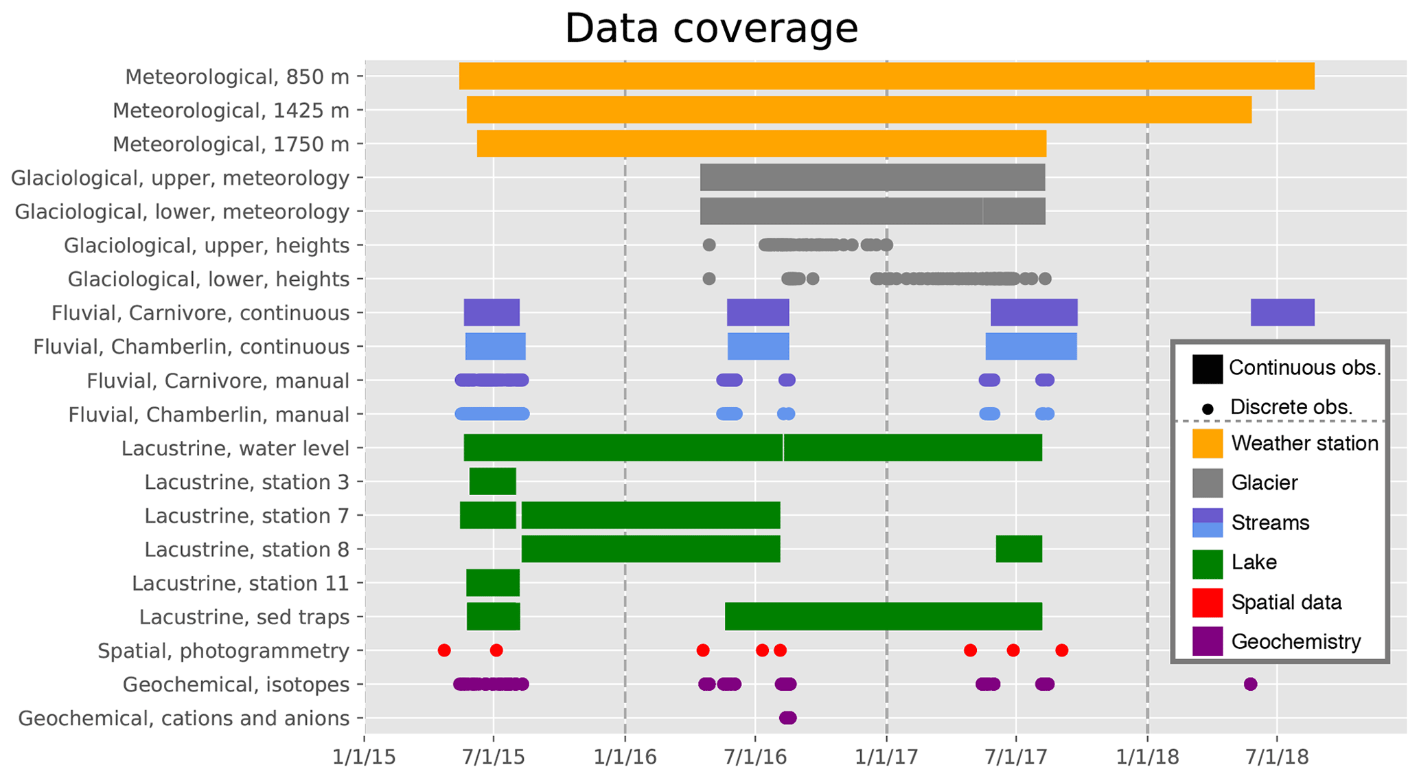
Figure 1Temporal coverage of data collected in the Lake Peters catchment. Data are either continuous hourly or bi-hourly observations (bars) or discrete observations in time (dots). Data are indicated as available if any variable is present for the given time. Observations and samples from sediment traps are not hourly but were collected over specific windows of time. The 1 January of each year is marked with a dotted line. Data collected from different parts of the Lake Peters catchment are shown with different colors in roughly the same order as they are discussed in Sect. 3. See Sect. 3 for a more detailed description of the data. Some data (Lake Peters TROLL casts and bathymetry) are not represented in this figure.
Our collection of meteorological, glaciological, fluvial, lacustrine, spatial, and geochemical data within the Lake Peters catchment can be used to quantify and explore interconnections in the local hydrologic system. Additionally, this multi-year monitoring study provides useful context for the interpretation of past environmental changes that can be inferred from lake sediments from Lake Peters (Benson, 2018; Benson et al., 2019). In the interest of making these unique and valuable data readily accessible to potential users, the objective of this paper is to document and describe the datasets, as well as data-collection methods, biases, and corrections.
Lake Peters (69.32∘ N, 145.05∘ W) lies at 853 m above sea level (m a.s.l.) on the north side of the Brooks Range, an east–west trending mountain range in Arctic Alaska (Fig. 2). The Brooks Range extends 1000 km, separating the Arctic coastal plain to the north from the Yukon Basin to the south. The third tallest peak in the range, Mount Chamberlin (2712 m a.s.l.; Nolan and DesLauriers, 2016) lies 3 km east of Lake Peters.
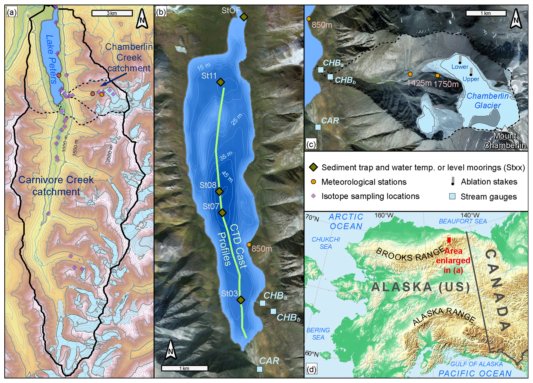
Figure 2(a) Lake Peters catchment (solid black boundary) and Carnivore Creek and Chamberlin Creek sub-catchments (dashed boundaries) with land-based observational locations. (b) Lake Peters bathymetry and lacustrine observational locations. (c) Chamberlin Creek sub-catchment and Chamberlin Glacier. (d) Brooks Range setting in Alaska and study area location.
One of the largest and deepest glacier-fed lakes in Arctic Alaska, Lake Peters has a maximum water depth of 52 m and an area of ∼6.4 km2. The lake's catchment (171 km2) has 9 % glacier coverage based on our aerial photography in 2016 and receives a majority of stream flow from Carnivore Creek, which has a 128 km2 catchment with 10 % glacier coverage (Fig. 2). The Carnivore catchment contains six glaciers exceeding 0.5 km2 in area and numerous smaller glaciers, with a median elevation for all glaciers of 1910 m a.s.l. The largest glacier (3.5 km2; 1410–2430 m a.s.l.) is situated at the head of Carnivore Creek. Since the Little Ice Age (late 19th century), the largest catchment glaciers have reduced in length by over 30 %. Lake Peters' secondary inflow, Chamberlin Creek, has a 8 km2 catchment that is 23 % covered by Chamberlin Glacier (1.7 km2; 1600–2710 m a.s.l.) (Fig. 2). The lake drains to the north into Lake Schrader, whose outflow, the Kekiktuk River, discharges into the Sadlerochit River and ultimately the Arctic Ocean. Lake Peters and Lake Schrader, or “Neruokpuk Lakes”, are ice covered from early October through mid-June or July and often thermally stratify (Hobbie, 1961). The basin is north of the modern tree line in a region underlain by continuous permafrost, with a thin active layer. Soils are rocky with thin tundra cover. Bedrock within the basin is Devonian–Jurassic sedimentary to meta-sedimentary rocks primarily of the Neruokpuk Formation (Reed, 1968).
Climate at Lake Peters is semi-continental, with temperatures more extreme than locations on the coastal plain. A short observational time series of weather from Lake Peters was initiated during the International Geophysical Year (Hobbie, 1962) and was summarized by March (2009). For May 2015–August 2018, measurements from weather stations installed in the Lake Peters basin indicate that average summer (JJA) temperature ranged from 6.3 to 7.7 ∘C, average winter (DJF) temperature ranged from −24 to −17.2 ∘C, and total summer rainfall was between 112.8 and 241.2 mm over the study period (Table 1). Strong temperature inversions develop during the winter, with differences as large as 15 ∘C between 850 and 1425 m a.s.l. Other key climate variables are summarized in Table 1.
Table 1Summary of key meteorological and hydrological variables observed in the Lake Peters watershed. DJF temperatures include December of the previous year. The number of extrapolated days for full-season discharge (Q) measurements refers to the number of late-season days for which flow occurred but was not measured by our instruments, and was therefore extrapolated using methods described in Sect. 3.3.2.
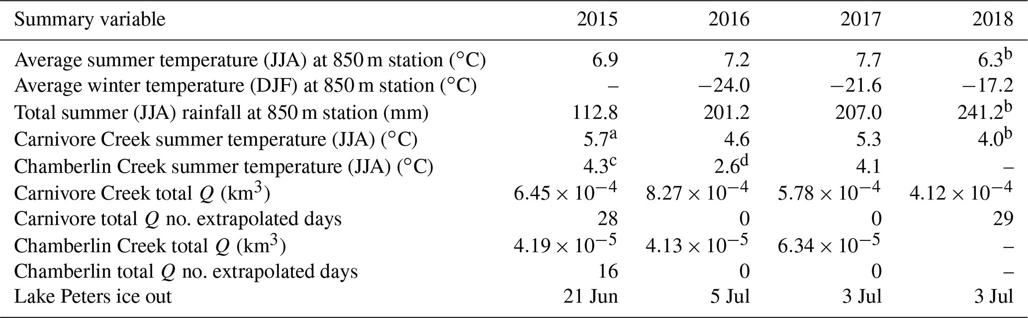
a 1 June–3 August. b 1 June–22 August. c 1 June–14 August. d 1–20 June and 8–17 August.
3.1 Meteorological data
Three weather stations operated in the Lake Peters catchment from May 2015 through August 2018 along an elevational gradient (Fig. 3) (Kaufman et al., 2019a). The lowest elevation station was mounted on the roof of the cabin at the research station at 850 m a.s.l. along the shoreline of Lake Peters. Additional stations were installed on tripods at 1425 m a.s.l. below the proximal flank of the Little Ice Age moraine of Chamberlin Glacier, and the highest elevation station was at 1750 m a.s.l. at the crest of the left lateral moraine of Chamberlin Glacier (Fig. 3).
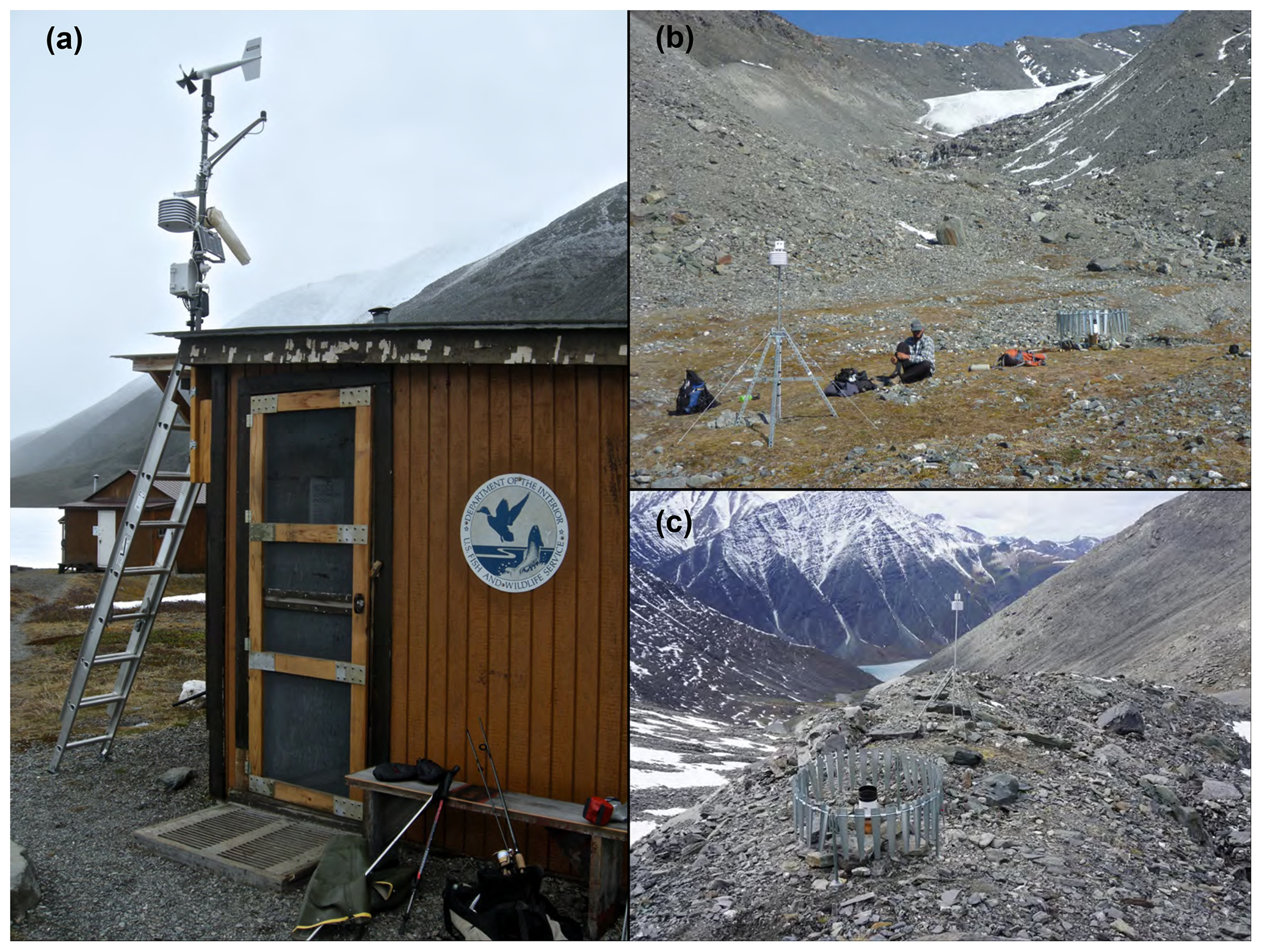
Figure 3Weather stations at (a) 850, (b) 1425, and (c) 1750 m a.s.l. in the Lake Peters watershed.
All three stations were equipped with air temperature and relative humidity sensors (Hobo Pro v2 Temp and RH sensors) and ground temperature sensors at 2 and 30 cm depth (Hobo Pro V2 2X with 184 cm (6 ft) extension). The 850 and 1425 m a.s.l. stations were equipped with backup air temperature and relative humidity sensors (Hobo Pro v2 Temp and RH sensors). All temperature and relative humidity sensors were housed in Hobo solar radiation shields. The 850 m a.s.l. station was additionally equipped with a barometer (Hobo barometric pressure sensor – S-BPB-CM50), an anemometer (Young wind monitor – 5103), and a pyranometer (solar radiation sensor – S-LIB-M003). At all three stations, tipping bucket rain gauges (Hobo rain gauge 0.2 mm with pendant – RG3-M) were installed on the ground away from the stations and equipped with Alter-type windshields to reduce wind-related undercatch. Correlations between daily precipitation recorded at 850 m a.s.l. with daily precipitation recorded at 1425 and 1750 m a.s.l. indicate that trends are coherent within the watershed with minimal (but expected) differences (Fig. 4).
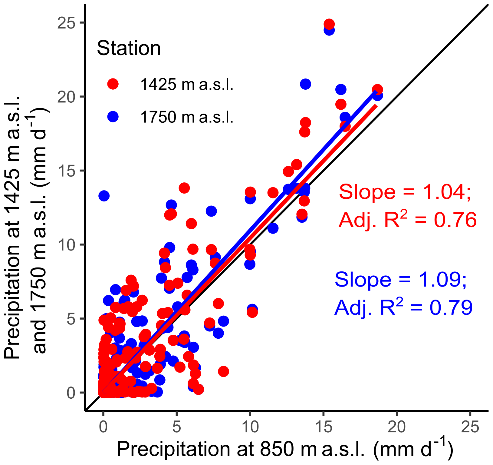
Figure 4Correlations between daily precipitation at 1425 m a.s.l. (red) and 1750 m a.s.l. (blue) with daily precipitation at 850 m a.s.l. Lines are least squares regressions. Also shown in black is the 1:1 line.
All three stations were generally continuously operational, though instrument failure caused gaps in the collection of some data from 21 September 2015 to 19 April 2016 at the 850 m a.s.l. station. Shorter instrument failures are documented for each sensor in the data files.
3.2 Glaciological data
The elevation of the surface of Chamberlain Glacier and its seasonal snow cover were observed using ablation stakes and interval photography (Geck et al., 2019). Graduated stakes were installed on 27 April 2016 at two sites along the lower part of the glacier: “lower” (69.29312∘ N, 144.93814∘ W; 1772 m a.s.l.) and “upper” (69.29031∘ N, 144.93134∘ W; 1860 m a.s.l.) (Fig. 5a). Photographs captured the exposed stake height using Wingscapes time-lapse cameras (SKU: WCT-00122) set to automatically record every 6 h. Ablation stake heights were observed on photographs (27 April 2016–11 August 2017) at a precision of 1 cm. Cameras were mounted on tripods constructed of electrical conduit (Fig. 5b). Air temperature sensors (Hobo Pro v2 Temp and RH sensors and/or Hobo pendant) housed in Hobo solar radiation shields recorded mean hourly temperatures 2 m above the snow surface at each site (Fig. 5b) (Kaufman et al., 2019b).
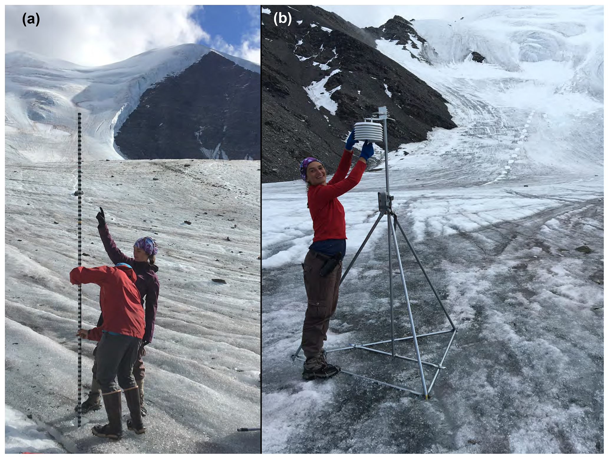
Figure 5Examples of (a) ablation stakes (lower site) and (b) weather stations (upper site) installed on Chamberlin Glacier.
3.3 Fluvial data
3.3.1 Field methods
Two hydrological stations were established in May 2015: one at Carnivore Creek (Schiefer et al., 2019a; Fig. 6a) and one at Chamberlin Creek (Schiefer et al., 2019b; Fig. 6b). At each station, an In-Situ TROLL 9500 (TROLL) was deployed during the open-channel season to measure pressure, temperature, conductivity, and turbidity, and a Hobo U20 water level logger was used for backup measurements of pressure and temperature. The instruments were attached to a cage constructed from aluminum tubing and chicken wire. A stage gauge was installed at each of the hydrological stations, and water level and reach conditions were captured in hourly photographs by field cameras. Cages were installed in thalwegs of stable reaches and loaded with boulders to resist movement (Fig. 6b). The field procedure was repeated for the 2016, 2017, and 2018 field seasons (May–August), though no instruments were successfully deployed in Chamberlin Creek in 2018, and only Hobo data (not TROLL) were recovered from Carnivore Creek in 2018.
In Carnivore Creek, the cage for the hydrological station was secured in the same location in all years in the thalweg of the main channel, near the outlet to Lake Peters, but upstream of where the channel anabranches on the alluvial plain (Fig. 6a). In contrast, in Chamberlin Creek, the location of the hydrological station was modified from year to year due to the difficulty of securing the TROLL and Hobo loggers to withstand the highest flood events of each field season. For 2015, the Hobo data provide a more complete record of water pressure measurements at Chamberlin Creek, and were therefore primarily used for the continuous time series. However, on 4 June the Hobo sensor failed and was re-established in a slightly different position on 5 June. The small shift in instrument position was corrected by comparing water pressure from the Hobo and TROLL and adjusting the early season Hobo water pressure from 5 June through the end of the season. Following these issues at Chamberlin Creek in 2015, the instruments were secured to channel-side bedrock in an upstream pool for the 2016 field season, but were ultimately carried downstream in the largest flood event of 2016 on 8 July. For the 2017 field season, the instruments were secured to a large boulder near the original 2015 hydrological station.
In addition to the continuous measurements from the TROLL and Hobo loggers, discrete discharge (Q) and suspended sediment concentration (SSC) measurements were taken using a hand-held Hach FH950 flow meter and a US DH-48 suspended sediment sampler, respectively, during the 2015, 2016, and 2017 field seasons. Discrete field sampling of discharge was most frequent and spanned the greatest range in 2015. In Carnivore Creek, discrete measurements were taken adjacent to the hydrological station using a cross section with a seasonally deployed tag line to measure consistent 1 m widths between observation points across the creek in the same location each year. In Chamberlin Creek, discrete measurements were primarily taken at the site of the 2015 hydrological station, though coordinates varied depending on the location of the instruments (described above).
3.3.2 Data analysis
Barometric pressure measurements from the 850 m a.s.l. meteorological station were used to convert instrument heights above the riverbed to stage. Discharge–stage regressions were used to construct continuous hourly discharge for the majority of the 2015 open-channel season in Carnivore and Chamberlin creeks (Fig. 7a–b). In Carnivore Creek, photographs of water level were imported to image viewing-and-analysis software to estimate 2.6 d of peak stage during a flood on 3 August 2015 (Fig. 7c) and its error margin. The regression used nine photographs selected to capture maximal water-level variability, and stage was established using a point-to-point method to capture temporal variability. In Chamberlin Creek, linear relations between stage from the Hobo and TROLL instruments permitted the compilation of a seamless discharge record for 2015 (Fig. 7d).
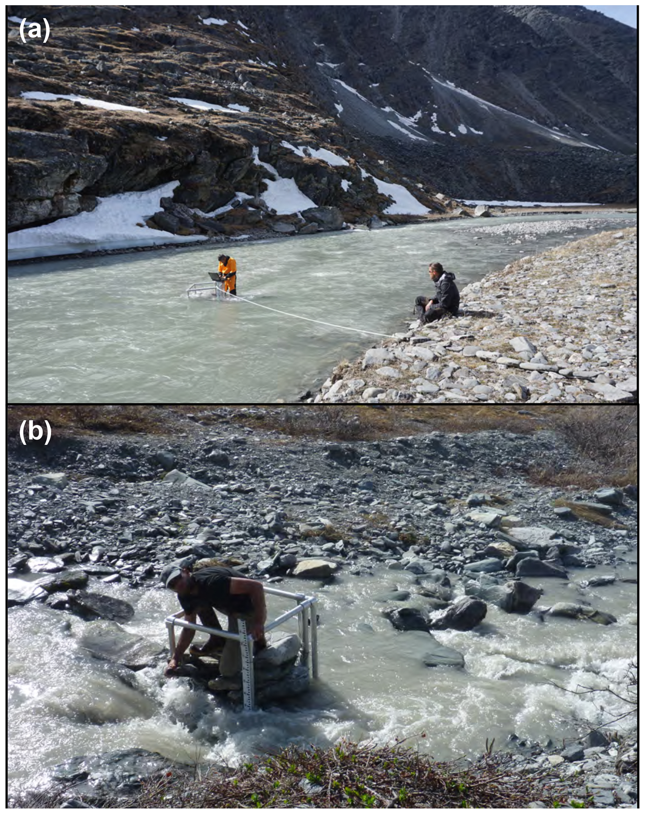
Figure 6Stream stage gauges for (a) Carnivore and (b) Chamberlin creeks. Instrumentation mounted in tubing is obscured by stage gauges.
For the 2016 open-channel season, alternative methods were applied due to the lack of velocity data required to compute discharge, assuming consistent discharge–stage relations between seasons (Thurston, 2017). To calculate continuous discharge for Carnivore Creek, stage was first regressed against cross-sectional area for both open-channel seasons separately (Fig. 7e). Stage for 2016 was then adjusted by the mean difference between 2015 and 2016 stage for the same data range for both years (Fig. 7e), to be consistent with 2015 stage by accounting for the shift in instrument positioning between years. The 2015 stage–discharge relation was then used to establish continuous discharge from stage measured in 2016 for that field season (Fig. 7a). The 2015 and 2016 stage data are remarkably consistent between seasons (Fig. 7e), and cross-sectional tag line and instruments were secured in the same locations in 2015 and 2016. However, there is potential for slightly different instrument positions between the two seasons, as well as for bed scour during the August 2015 flood. Therefore, while these data provide a reasonable estimate of 2016 discharge at Carnivore Creek, they do not conform to the standard procedure of obtaining a new rating curve for each season and are therefore considered approximate.
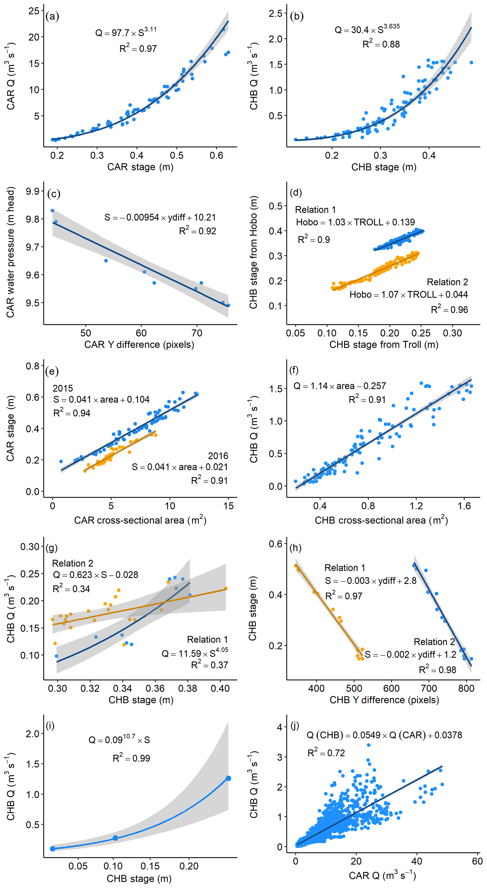
Figure 7Regression relations and associated confidence bands used to create continuous discharge (Q) time series throughout the 2015–2018 open-channel seasons in Carnivore (CAR) and Chamberlin (CHB) creeks. (a) Discharge – stage (S) relation for CAR (2015); (b) discharge – stage relation for CHB (2015); (c) water-pressure (from TROLL) – vertical difference (y diff; shown on photographs) relation for CAR (2015); (d) relations of stage calculated from Hobo U20 water pressure against stage calculated from TROLL 9500 water pressure for CHB (both 2015); (e) stage – cross-sectional area linear relation for CAR (2015 and 2016); (f) discharge – cross-sectional area linear relation for CHB (2015); (g) discharge – stage (from Hobo) power relation for CHB (2016); (h) stage – vertical difference (y diff; shown on photographs) linear relations for CHB (both 2016); (i) discharge – stage exponential relation for CHB (2016); and (j) relation of discharge in CHB against discharge in CAR with a 2 h lag (2015 and 2016). Refer to Thurston (2017) for additional information.
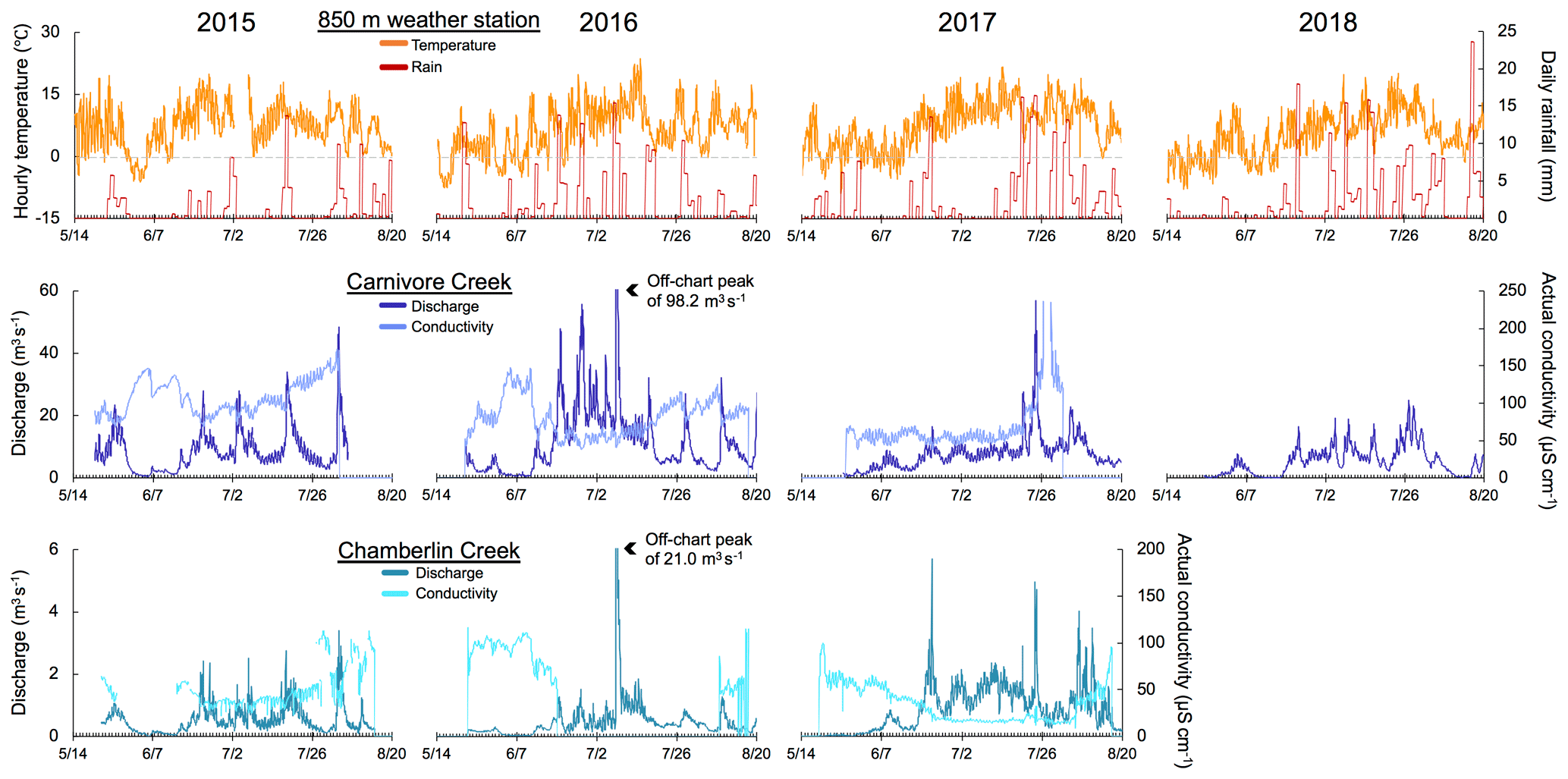
Figure 8Time series of hourly air temperature and rainfall from the 850 m a.s.l. weather station at Lake Peters shown alongside conductivity and discharge for Carnivore and Chamberlin creeks, 2015–2018. The gray line in the top row indicates 0 ∘C.
The Chamberlin Creek data for 2016 are also approximate due to both the lack of a new rating curve for this season and the unconventional methods used to calculate continuous discharge. The method used for Carnivore Creek could not be applied to Chamberlin Creek because the TROLL and Hobo instruments were secured in different locations between 2015 and 2016. Instead, 2015 discharge was regressed against cross-sectional area (Fig. 7f), and this relation was then used to construct discrete 2016 extrapolated discharges sampled from 2016 cross-sectional areas. These discharge–stage relations were used to calculate continuous discharge for 2016 until a flood event that began on 20 June (Fig. 7g) washed the instruments downstream. Several methods were used to construct stage and discharge following this flood (Fig. 7h–j). These methods included photographs of river level from time-lapse cameras (46 d of discharge values); a regression of Chamberlin Creek and Carnivore Creek discharges using all available data (3.6 d); and a three-point stage–discharge rating curve sampled downstream of the rating curve applied prior to the flood (8.8 d). When none of the aforementioned alternatives were possible, gaps were interpolated, amounting to a total of five gaps that range from 2 to 19 h. The majority of the 2016 stage record (20 June–5 August 2016) was estimated for Chamberlin Creek from photographs of water levels (Fig. 7h; Thurston, 2017). Water levels were measured using two reference points on a total of 13 photographs, then regressed separately against discharge. The first reference point was suitable for most discharges but was not accurate after 16 July 2016 when water levels dropped low enough to expose a small bar. The second reference point was suitable for low discharges but overtopped during high flows. Error was conservatively 10–20 image pixels, where 10 pixels equate to an approximately 0.14 m3 s−1 error margin in either direction from the average discharge of 0.72 m3 s−1. For the peak of the flood event on 8 July at 02:00 GMT−9, error is estimated to be 100 pixels in either direction because water level and control points were obscured (equating to a maximum error range of 7.31 to 49 m3 s−1 for the peak discharge of 21 m3 s−1). The Chamberlin Creek hydrological station was ultimately re-established in a new location, and a new rating curve was used to reconstruct discharge from 8 August 2016 at 18:00 until 17 August 2016 at 13:00 (Fig. 7i). Where no discharge–stage rating curves or photographs were available, the relation between Carnivore Creek and Chamberlin Creek discharges was used (Fig. 7j). The photographic method was favored whenever photographs were available to keep the sub-catchment discharge records independent. Considerable scatter between Carnivore and Chamberlin Creek discharge records is attributed to hydrological differences between the sub-catchments (Fig. 7j).
Stage–discharge rating curves developed from 2015 and 2016 data were used to convert continuous stage records to discharge for Carnivore Creek for 2017 and 2018, and for Chamberlin Creek for 2017. Adjustments were made to account for changes in instrumentation position relative to the channel bed. The 2017 and 2018 data for Carnivore Creek and the 2017 data for Chamberlin Creek are therefore also considered approximate. While the limitations of the discharge data are recognized, they are still valuable indicative records of hydrological conditions in this remote Arctic setting, where few such datasets exist. Summarized discharge data alongside meteorological data at the 850 m a.s.l. station are shown in Fig. 8.
To estimate the full hydrologic season discharge volumes (Table 1), the continuous Carnivore and Chamberlin Creek time series required extrapolation to include the relatively low late-season flows following removal of instruments. Mean daily discharge for this period was estimated based on the relation between Carnivore and Chamberlin creeks and the nearby Hula Hula River, which explains almost half the variability in our study creeks in the late season.
3.4 Lacustrine data
3.4.1 Limnological data
Hourly water-level measurements were taken using Hobo U20L water level loggers installed on anchored moorings near the water's surface at two locations in Lake Peters: one in its central basin and one near its outflow (Fortin et al., 2019a). Pressure data were corrected to water depth using barometric pressure measurements from the 850 m a.s.l. meteorological station.
In 2015, a series of TROLL casts were taken to measure temperature, turbidity, and conductivity profiles at stations along a north–south transect throughout Lake Peters (Fortin et al., 2019b). These casts were performed at a varying number of stations on a total of 33 d over the course of the field season.
In 2015, 2016, and 2017, lake temperature and luminous flux data were collected at various water depths on anchored moorings throughout the lake (Fig. 2) (Kaufman et al., 2019c). The moorings were equipped with Hobo pendants and Hobo Water Temp Pro loggers at different water depths to monitor the thermal structure of the lake. Moorings located in the central basin of the lake were deployed from May 2015 until August 2016 (Station 7) and August 2015 until August 2017 (Station 8). A mooring in the distal basin (Station 11) was deployed from May 2015 to August 2015, and a mooring in the proximal basin (Station 3) was deployed from May 2015 until August 2015.
3.4.2 Sediment trap data
Throughout 2015–2017, sediment traps were deployed in Lake Peters to measure the rate of deposition and to collect suspended sediments in the lakes (Kaufman et al., 2019d). In 2015, three pairs of static (i.e., non-automated) traps with different aspect ratios (different collection tube heights but same collection tube diameters) (Fig. 9a) were deployed from May to August at a central location of Lake Peters to determine the effect of these proportions on sediment collection efficiency. From May to August 2016 and again from August 2016 through August 2017, one static trap was deployed in Lake Peters. This trap consisted of 50 mL centrifuge tubes attached to the mouths of inverted 2 L plastic bottles (beverage containers) with the bottoms removed (to funnel sediments into the tubes) (Fig. 9b). Each trap comprised two or three replicate tubes and bottles deployed at different depths along an anchored mooring. In addition, an incrementing sediment trap described by Muzzi and Eadie (2002) was deployed from May 2016 through August 2017, collecting sediments in 23 bottles rotating over daily to weekly increments (Fig. 9c).
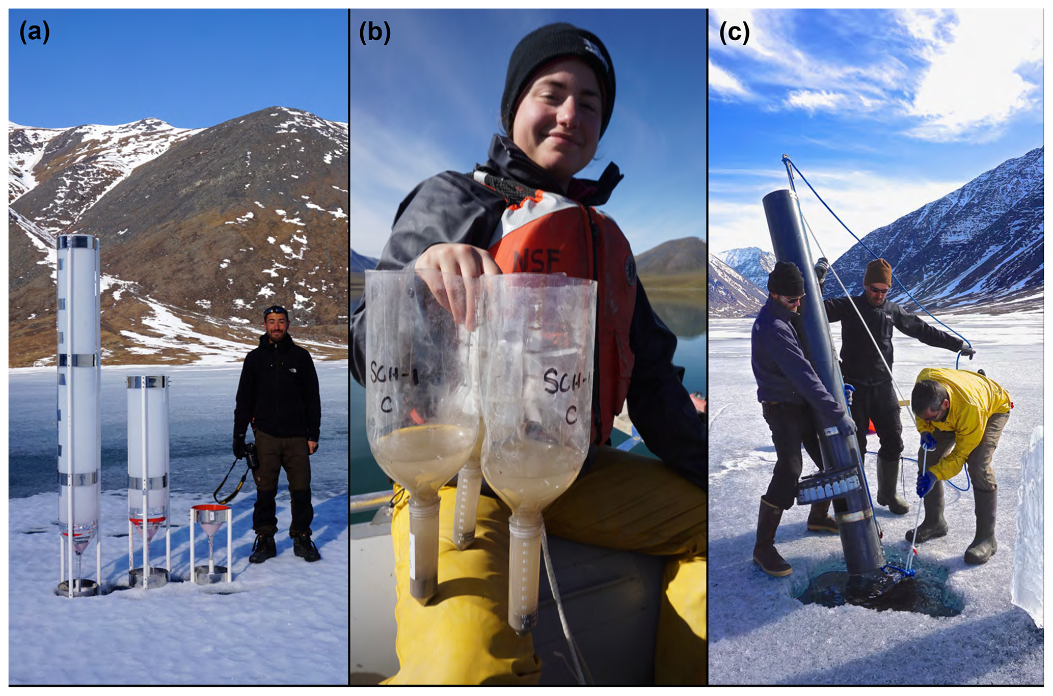
Figure 9Examples of the types of sediment traps installed in Lake Peters: (a) static traps used to investigate the effect of collection-tube aspect ratio, (b) 2 L bottle static traps upon retrieval, and (c) installation of an incrementing trap.
For all sediment samples, dry sediment mass, daily flux, and annual flux were calculated. For several static trap samples, grain-size data (mean, standard deviation, d50, d90 and percentages of sand, silt, and clay) were determined using a Coulter LS-320. Samples were pretreated with 30 % H2O2 and heated overnight at 50 ∘C to remove organic material, and then treated with 10 % Na2CO3 for 5 h to remove biogenic silica. Pretreated samples were deflocculated by adding sodium hexametaphosphate and shaking for 1 h before performing grain-size analysis. Organic-matter content for some samples was determined using loss-on-ignition analysis.
3.5 Spatial data
3.5.1 Bathymetry
Bathymetric data were collected using a Lowrance Elite-5 HDI Combo sonar depth recorder along several transects throughout Lake Peters in August 2015 (Schiefer et al., 2019c). These data were used to create a bathymetric map with ArcGIS 9.1.
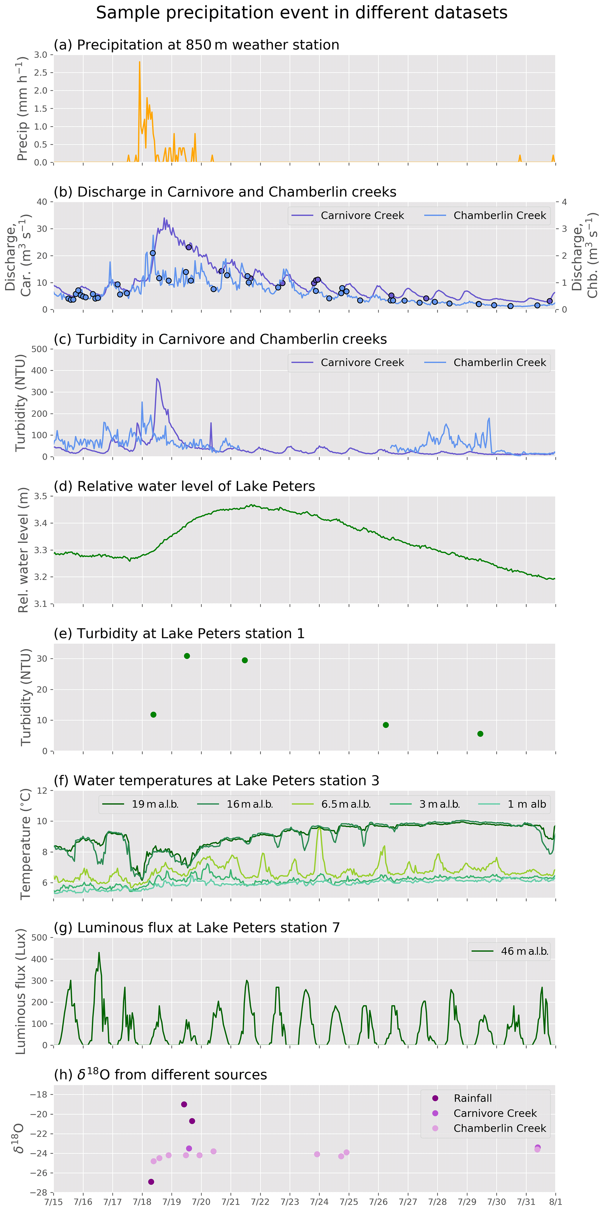
Figure 10An example of a complementary dataset from Lake Peters observatory, tracing the effects of a precipitation event in July 2015. (a) Rainfall at the 850 m a.s.l. station; (b) Carnivore Creek and Chamberlin Creek discharge and (c) turbidity; (d) Lake Peters relative water level; (e) maximum turbidity at Lake Peters station 1; (f) water temperatures at different heights above lake bottom (a.l.b.) at Lake Peters station 3; (g) luminous flux at Lake Peters Station 7; and (h) δ18O at different sites. To complement panel (e), a more detailed sample of turbidity data is shown in Fig. 11.
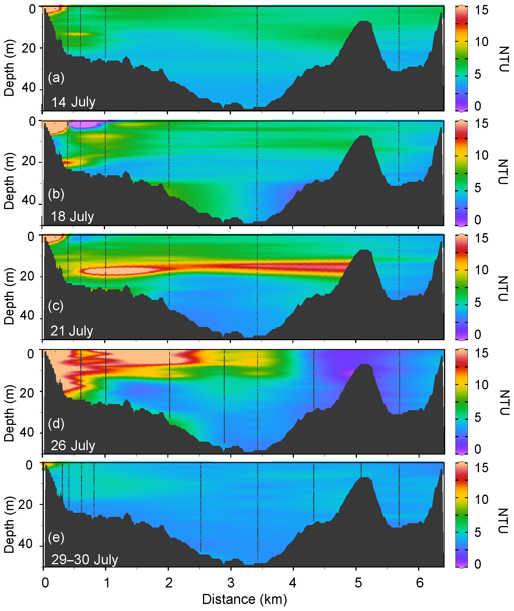
Figure 11Turbidity in Lake Peters over the course of a precipitation event in July 2015; turbidity data are shown for (a) 14 July, (b) 18 July, (c) 21 July, (d) 26 July, and (e) 29 and 30 July (composite). Black shading indicates lake bathymetry, and black dashed lines indicate locations of TROLL casts. The x axis indicates north–south distance across the lake from the outflow of Carnivore Creek. Figure created using Ocean Data View (ODV) software.
3.5.2 High-resolution photogrammetry
Airborne photogrammetric data were acquired two times in 2015 (23 April and 5 July), three times in 2016 (19 April, 11 July, and 5 August), and three times in 2017 (28 April, 27 June, and 3 September) (Nolan, 2019). These data were used to create digital elevation models (DEMs), with a horizontal resolution of 50–80 cm provided in NAD83(2011) NAVD88 Geoid 12B. When conditions permitted (23 April 2015; 5 July 2015; 19 April 2016; 28 April 2017), imagery of the entire Carnivore Creek watershed was acquired. On all other dates, only the eastern side of the valley, where the catchment glaciers are located, was captured. These data were acquired using a Nikon DSLR attached to a survey grade Global Navigation Satellite System (GNSS) on board a manned aircraft, providing photo-center position to 10 cm or better and thus eliminating the need for ground control. Accuracy within this steep mountain environment was found to exceed 20 cm horizontally and vertically (Nolan and DesLauriers, 2016), without the use of ground control. Data acquisition methods are described in detail in Nolan et al. (2015). These DEMs were used to create difference DEMs that can be used to measure snowpack thickness throughout the entire watershed as well as glacier surface elevation change. The accuracy of these DEM-derived snow thickness measurements has previously been found to be comparable to those acquired using hand-operated probes (Nolan et al., 2015). However, larger errors are expected in rugged mountain topography, as the 50 cm DEMs cannot resolve many small crenulations, likely causing some spatial biasing.
3.6 Geochemical data
A total of 187 water samples were collected from the Lake Peters catchment between 2015 and 2018 and analyzed for isotopes of oxygen (δ18O) and hydrogen (δD) measured as deviation from the Vienna Standard Mean Ocean Water standard (‰ VSMOW) (Kaufman et al., 2019e). These data, combined with conductivity measurements, were input to a hydrograph mixing model to estimate the relative contributions of various water sources to Carnivore and Chamberlin creeks (Ellerbroek, 2018). Sampling intervals varied by location but were approximately every 2–6 d when a field team was present. In one 24 h period in August 2016, each creek was sampled every 2 h using a Teledyne ISCO 3700 portable automatic water sampler (ISCO). These ISCO samples from Carnivore and Chamberlin creeks were also analyzed for major cation and anion geochemistry using a Dionex ICS-3000 ion chromatograph with an analytical precision of ±5 % (Kaufman et al., 2019e). Water samples were also collected from three unnamed glaciated tributaries in the Carnivore Creek valley and from three unnamed non-glacial streams that intermittently drain into Lake Peters. All samples were collected in 10 mL polyethylene bottles rinsed three times with sample water.
Winter precipitation samples were collected from multiple locations. Twenty-seven snowpack samples were collected with snow density measurements in April 2016 and May 2017 at a variety of depths from 21 snow cores along an elevational gradient. Samples of glacial melt, glacial ice, and snow drifts were collected over 2015 and 2016. All snow and ice samples were collected in airtight plastic bags and transferred into rinsed 10 mL polyethylene bottles after melting. Rain samples were collected sporadically after storm events from spill off from the roof of the G. William Holmes research station and transferred into rinsed 10 mL polyethylene bottles.
Following each field season, water samples were processed using wavelength-scanned cavity ring-down spectroscopy. Analytical precision is approximately 0.3 ‰ for δ18O and 0.8 ‰ for δD (Los Gatos Research, 2018).
4.1 Data example: tracing an event through the Lake Peters glacier–river–lake system
To examine how precipitation works its way through the Lake Peters catchment system, and to depict a small subset of the available data, multiple datasets are shown for a precipitation event in the latter half of July 2015 (Figs. 10, 11). During this event, the 850 m a.s.l. meteorological station recorded a total rainfall of 22.4 mm between 17 and 20 July (Fig. 10a). In response, hydrological stations at both Carnivore and Chamberlin creeks recorded an increase in discharge to Lake Peters, with Carnivore Creek discharge reaching far higher values due to its larger catchment (Fig. 2). Discharge then decreased over several weeks, long after the precipitation event concluded, with diurnal fluctuations illustrating the effect of glacier melt (Fig. 10b). Turbidity increased in both creeks, coincident with the beginning of elevated discharge (Fig. 10c). The influx of water raised the water level of Lake Peters, which lagged, likely as a function of the total integration of new water as well as outflow into Lake Schrader (Fig. 10d). This event had several additional effects on the water of Lake Peters: turbidity increased during the event (Fig. 10e), the inflow of water caused a temporary drop in water temperatures closer to the lake surface (Fig. 10f), and the amount of luminous flux a few meters below the water's surface dropped (Fig. 10g). Isotopic values were also recorded from rainfall and creek water at several times during this event (Fig. 10h).
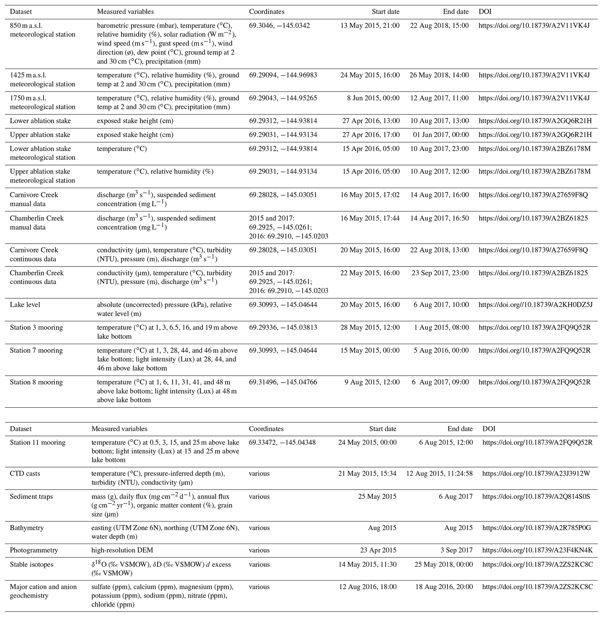
Table 2Observational datasets generated by the Lake Peters observatory instrumentation and archived at the NSF Arctic Data Center. All observations are reported for the time zone GMT-9
To quantify the spatial characteristics of the sediment pulse entering Lake Peters during this precipitation event, data from TROLL casts taken throughout the lake on multiple days before, during, and after the event were examined (Fig. 11). These data indicate that the spatial pattern of turbidity anomalies throughout Lake Peters is more complex than that captured at a single, proximal station shown in Fig. 10e.
This multifaceted perspective of a precipitation event represents only a small fraction of the total data produced by this field effort, but illustrates both the interconnectedness of processes in the Lake Peters catchment and the potential for these datasets to further our understanding of Arctic weather–glacier–river–lake systems dynamics.
4.2 Modeling applications
In addition to exploring interactions between components of the catchment, a major goal of acquiring these datasets is to support Earth system modeling efforts in the watershed and region, where such field-based observational data are rare. The datasets are well suited to serve as input data or calibration targets for hydrologic modeling and fluvial sediment transport models. Basin-scale distributed hydrologic modeling is ongoing, but it is limited by the sparse data available. Although meteorological input data were measured at three sites spanning 900 m in elevation, the catchment for Carnivore Creek is large, and precipitation in the southern part of the basin is not well constrained. A hydrological balance was developed, and a hydrograph mixing model, used to quantify the relative proportion of different source waters, was calibrated using the discharge, geochemistry and runoff data (Ellerbroek, 2018). For sediment-flux modeling, discharge, turbidity, and suspended sediment concentration datasets were used to develop empirical sediment transport models (Thurston, 2017).
A major limitation is the year-to-year variability in these data. Modeling endeavors for the catchment would benefit from continued observations and should be supplemented with comparison from longer-term datasets, perhaps most notably from McCall Glacier (Nolan et al., 2005; Klein et al., 2016), Toolik Lake (Hobbie et al., 1995), and climate reanalysis products (Auger et al., 2018).
All DOI-referenced datasets described in this paper are archived at the National Science Foundation Arctic Data Center at the following overview web page for the project: https://arcticdata.io/catalog/view/urn:uuid:df1eace5-4dd7-4517-a985-e4113c631044 (last access: 13 October 2019; Kaufman et al., 2019f). Datasets are available for download (Table 2) as CSV files (or TIFFs for photogrammetry data), with accompanying metadata including an abstract, key words, methods, spatial and temporal coverage, and personnel information pertinent to each dataset.
The meteorological, glaciological, fluvial, and lacustrine datasets from Lake Peters and its catchment presented in this paper offer a unique and valuable opportunity to study an Arctic glacier-fed lake system. The observational data have contributed to our understanding of individual events as well as intra- and inter-annual variability within this catchment. By making these data available, we hope to foster a more detailed understanding of the processes leading to sedimentation in Arctic lake catchments. Furthermore, these data may provide important context for interpretation of lake sediment records from this study region and elsewhere, as well as for hydrological and sedimentological modeling studies.
ES, NPM, DF, JG, MGL, MN, and DSK developed the observational design. EB, LLT, ES, NPM, DF, JG, MGL, MN, SHA, CWB, RAE, CCR, and DSK led installation, development and/or curation of components of the observations. EB, LLT, ES, NPM, JG, MPE, CW, AJW, and DSK wrote the original paper. EB, LLT, ES, NPM, DF, SHA, RAE, MPE, CW, and AJW produced figures for the paper. EB, DF, and DSK curated the datasets at the NSF Arctic Data Center. All authors provided minor edits to the text of the final paper.
The authors declare that they have no conflict of interest.
Datasets from the Lake Peters watershed were collected with the help of numerous field assistants, including Zak Armacost, Mindy Bell, Ashley Brown, Anne Gädeke, Jeff Gutierrez, Rebecca Harris, Stacy Kish, Lisa Koeneman, Anna Liljedahl, Maryann Ramos, Doug Steen, and Ethan Yackulic. Sedimentary grain-size data were processed with assistance from Daniel Cameron and Katherine Whitacre. Water isotope analyses were performed with assistance from Jamie Brown at NAU's Colorado Plateau Stable Isotope Facility, and major cation and anion analyses were performed by Tom Douglas of the U.S. Army Cold Regions Research and Engineering Laboratory. We thank the U.S. Fish and Wildlife Service – Arctic National Wildlife Refuge for use of the G. William Holmes research station and for permitting our research; Polar Field Services, Inc./CH2M Hill for support and outfitting while in the field; Dirk Nickisch and Danielle Tirrell of Coyote Air for safely flying our field teams to and from Lake Peters; LacCore/CSDCO for assistance with processing and archiving of sedimentary sequences from Lake Peters; and PolarTREC for a productive partnership that contributed greatly to the broader impacts of this project.
This research has been supported by the National Science Foundation (grant nos. 1418000, 1418032, and 1418274).
This paper was edited by Prasad Gogineni and reviewed by two anonymous referees.
Auger, J., Birkel, S., Maasch, K., Mayewski, P., and Schuenemann, K.: An ensemble mean and evaluation of third generation global climate reanalysis models, Atmosphere, 9, 1–12, https://doi.org/10.3390/atmos9060236, 2018.
Benson, C. W.: 16,000 Years of Paleoenvironmental Change from the Lake Peters-Schrader Area, Northeastern Brooks Range, Alaska, M.S. thesis, Northern Arizona University, Flagstaff, Arizona, USA, AAT 10812107, 2018.
Benson, C. W., Kaufman, D. S., McKay, N. P., Schiefer, E., and Fortin, D.: A 16,000 year-long sedimentary sequence from Lake Peters and Schrader (Neruokpuk Lakes), northeastern Brooks Range, Alaska, Quaternary Res., 1–17, https://doi.org/10.1017/qua.2019.43, 2019.
Ellerbroek, R. A.: Three Component Hydrograph Separation for the Glaciated Lake Peters Catchment, Arctic Alaska, M.S. thesis, School of Earth and Sustainability, Northern Arizona University, Flagstaff, Arizona, USA, ProQuest ID 2112380481, 2018.
Fortin, D., Kaufman, D. S., Schiefer, E., Thurston, L. L., Geck, J., Loso, M. G., McKay, N. P., Liljedahl, A., and Broadman, E.: Lake Peters water level, Arctic National Wildlife Refuge, Alaska, 2015–2017, https://doi.org/10.18739/a2kh0dz5j, 2019a.
Fortin, D., Schiefer, E., Thurston, L. L., Kaufman, D. S., Geck, J., Loso, M. G., McKay, N. P., Liljedahl, A., and Broadman, E.: CTD casts (conductivity, temperature, depth) in Lake Peters, Arctic National Wildlife Refuge, Alaska, 2015, https://doi.org/10.18739/a23j3912w, 2019b.
Geck, J., Loso, M. G., Schiefer, E., Thurston, L. L., McKay, N. P., Kaufman, D. S., Fortin, D., Liljedahl, A., and Broadman, E.: Ablation stake data from Chamberlin Glacier, Arctic National Wildlife Refuge, Alaska, 2016–2017, https://doi.org/10.18739/a2gq6r21h, 2019.
Hobbie, J. E.: Summer temperatures in Lake Schrader, Alaska, Limnol. Oceanogr., 6, 326–329, https://doi.org/10.4319/lo.1961.6.3.0326, 1961.
Hobbie, J. E.: Limnological cycles and primary productivity of two lakes in the Alaskan Arctic, Ph.D. thesis, Department of Zoology, Indiana University, Bloomington, Indiana, USA, 1962.
Hobbie, J. E., Deegan, L. A., Peterson, B. J., Rastetter, E. B., Shaver, G. R., Kling, G. W., O'Brien, W. J., Chapin, F. T., Miller, M. C., Kipphut, G. W., and Bowden, W. B.: Long-term measurements at the arctic LTER site. In Ecological time series (391–409), Springer, Boston, MA, 1995.
Kaufman, D. S., Fortin, D., Schiefer, E., Thurston, L. L., Geck, J., Loso, M. G., McKay, N. P., Liljedahl, A., and Broadman, E.: Meteorological data from the Lake Peters watershed, Arctic National Wildlife Refuge, Alaska, 2015–2018, https://doi.org/10.18739/a2v11vk4j, 2019a.
Kaufman, D. S., Geck, J., Loso, M. G., Schiefer, E., Thurston, L. L., McKay, N. P., Fortin, D., Liljedahl, A., and Broadman, E.: Meteorological data from Chamberlin Glacier, Arctic National Wildlife Refuge, Alaska, 2016–2017, https://doi.org/10.18739/a2bz6178m, 2019b.
Kaufman, D. S., Fortin, D., Schiefer, E., Thurston, L. L., Geck, J., Loso, M. G., McKay, N. P., Liljedahl, A., and Broadman, E.: Lake Peters water temperature and luminous flux, Alaska, 2015–2017, https://doi.org/10.18739/a2fq9q52r, 2019c.
Kaufman, D. S., Fortin, D., Schiefer, E., Thurston, L. L., Geck, J., Loso, M. G., McKay, N. P., Liljedahl, A., and Broadman, E.: Sediment trap data from Lake Peters and Lake Schrader, Arctic National Wildlife Refuge, Alaska, 2015–2017, https://doi.org/10.18739/a2q814s0s, 2019d.
Kaufman, D. S., Ellerbroek, R. A., Fortin, D., Schiefer, E., Thurston, L. L., Geck, J., Loso, M. G., McKay, N. P., Liljedahl, A., and Broadman, E.: Geochemical and stable isotope composition data from precipitation, runoff, snow and ice collected in Lake Peters watershed, Arctic Wildlife Refuge, Alaska, 2015–2018, https://doi.org/10.18739/a2zs2kc8c, 2019e.
Kaufman, D. S., Fortin, D., Schiefer, E., Thurston, L. L., Geck, J., Loso, M. G., McKay, N. P., Liljedahl, A., Broadman, E., Benson, C. W., Nolan, M., and Ellerbroek, R. A.: Collaborative research: Developing a System Model of Arctic Glacial Lake Sedimentation for Investigating Past and Future Climate Change, Arctic Data Center, https://arcticdata.io/catalog/view/urn:uuid:df1eace5-4dd7-4517-a985-e4113c631044 (last access: 13 October 2019), 2019f.
Klein, E. S., Nolan, M., McConnell, J., Sigl, M., Cherry, J., Young, J., and Welker, J. M.: McCall Glacier record of Arctic climate change: Interpreting a northern Alaska ice core with regional water isotopes, Quaternary Sci. Rev., 131, 274–284, https://doi.org/10.1016/j.quascirev.2015.07.030, 2016.
Los Gatos Research: available at: http://www.lgrinc.com, last access: 22 July 2018.
March, J. R.: Synoptic climatology of the eastern Brooks Range, Alaska: a data legacy of the International Geophysical Year, M.S. thesis, Department of Atmospheric Science, University of Alaska, Fairbanks, Alaska, USA, 2009.
Muzzi, R. W. and Eadie, B. J.: The design and performance of a sequencing sediment trap for lake research, Mar. Technol. Soc. J., 36, 2–28, https://doi.org/10.4031/002533202787914025, 2002.
Nolan, M.: High resolution photogrammetric data of Chamberlin Glacier and the Lake Peters watershed, Alaska, 2015–2017, https://doi.org/10.18739/A23F4KN4K, 2019.
Nolan, M. and DesLauriers, K.: Which are the highest peaks in the US Arctic? Fodar settles the debate, The Cryosphere, 10, 1245–1257, https://doi.org/10.5194/tc-10-1245-2016, 2016.
Nolan, M., Arendt, A., Rabus, B., and Hinzman, L.: Volume change of McCall glacier, arctic Alaska, USA, 1956–2003, Ann. Glaciol., 42, 409–416, https://doi.org/10.3189/172756405781812943, 2005.
Nolan, M., Larsen, C., and Sturm, M.: Mapping snow depth from manned aircraft on landscape scales at centimeter resolution using structure-from-motion photogrammetry, The Cryosphere, 9, 1445–1463, https://doi.org/10.5194/tc-9-1445-2015, 2015.
Reed, B.: Geology of the Lake Peters area northeastern Brooks Range, Alaska, U.S. Geol. Surv. Bulletin 1236, 132 pp., 1968.
Schiefer, E., Thurston, L. L., Kaufman, D. S., Geck, J., Loso, M. G., McKay, N. P., Fortin, D., Liljedahl, A., and Broadman, E.: Carnivore Creek discharge and suspended sediment concentration, Alaska, 2015–2018, https://doi.org/10.18739/A27659F8Q, 2019a.
Schiefer, E., Thurston, L. L., McKay, N. P., Kaufman, D. S., Fortin, D., Geck, J., Loso, M. G., Liljedahl, A., and Broadman, E.: Chamberlin Creek discharge and suspended sediment concentration, Alaska, 2015–2017, https://doi.org/10.18739/A2BZ61825, 2019b.
Schiefer, E., McKay, N. P., Kaufman, D. S., Fortin, D., Geck, J., Loso, M. G., Liljedahl, A., and Broadman, E.: Bathymetric map of Lake Peters, Alaska, 2015, https://doi.org/10.18739/a2r785p0g, 2019c.
Thurston, L. L.: Modeling Fine-grained Fluxes for Estimating Sediment Yields and Understanding Hydroclimatic and Geomorphic Processes at Lake Peters, Brooks Range, Arctic Alaska, M.S. thesis, Northern Arizona University, Flagstaff, Arizona, USA, ProQuest ID 2025947690, 2017.