Relative sea level is defined as the height of the ocean water column bounded by two surfaces: solid Earth surface and sea surface. Change in relative sea level, ΔS, at a geographical location described by colatitude and longitude (θ,ϕ) over the time interval Δt may be expressed as follows:

where ΔN and ΔU are corresponding changes in sea-surface height and bedrock elevation, respectively. Both of these variables are usually expressed relative to the reference ellipsoid, which in turn is defined relative to either the center-of-mass (CM) of the total Earth system or the center-of-figure (CF) of the solid Earth surface. Tide gauges provide direct measurements of ΔS, whereas satellite altimetry measures ΔN in the CM reference frame.

Mass redistributed on Earth's surface provides a direct perturbation to the Earth's gravitational and rotational potentials, causing a corresponding perturbation in the geoid height. Since the geoid height on a realistic Earth does not necessarily have to coincide with the sea-surface height, we write

where ΔΦ is the net perturbation in Earth's surface potential, ΔC is a spatial invariant that explains the discrepancy between the sea-surface height and geoid height (Tamisiea, 2011), measured with respect to the same reference ellipsoid, and g is the mean gravitational acceleration at Earth's surface. As will be further discussed in Sect. 3, ΔC is essential to conserve mass. Space-based gravity missions, such as GRACE and GRACE Follow-On (GRACE-FO), provide direct measurements of the non-rotational part of ΔΦ (to be defined explicitly in Sect. 3) in the CM frame; the satellite system cannot measure the rotational part of ΔΦ because it retrieves data in an inertial reference frame.

In geodetic applications, global field variables are typically expanded in a spherical harmonic (SH) domain. Most of the GRACE data processing centers – including the University of Texas Austin's Center for Space Research (CSR), GeoForschungsZentrum Potsdam (GFZ), and Jet Propulsion Laboratory (JPL) – provide monthly solutions for normalized SH coefficients of the gravitational potential termed “Stokes coefficients”. Stokes coefficient anomalies – the values that deviate from the mean (static) field – can be used to readily retrieve changes in on-land ice and water storage or ocean bottom pressure. The goal of this paper is to provide Stokes coefficient anomalies (i.e., SH coefficients of ΔΦ minus rotational centrifugal potential) associated with the sea-level fingerprint of monthly changes in on-land ice and water storage, which are derived from CSR, GFZ, and JPL GRACE Stokes coefficients themselves. As we shall further clarify below, we provide these new fingerprint coefficients and their corresponding spatial maps computed in both CM and CF reference frames, with and without rotational feedback included. We also provide solutions for change in relative sea level ΔS and bedrock elevation ΔU. Corresponding solutions for sea-surface height, ΔN, may be retrieved using Eq. (1). For brevity, we hereafter drop the Δ symbol and assume that variables imply “change” in respective fields – not the absolute fields – implicitly.

Here we briefly summarize the fundamental concept and a numerical technique of solving the so-called “sea-level equation”. Much of the background and supporting materials may be found, for example, in Farrell and Clark (1976), Mitrovica and Peltier (1991), Adhikari et al. (2016), and Spada (2017). Let $L(\mathit{\theta },\mathit{\varphi },t)$ be the global, mass-conserving load function so that

where $H(\mathit{\theta },\mathit{\varphi },t)$ is the on-land change in water equivalent height over the time period t, and $S(\mathit{\theta },\mathit{\varphi },t)$ is the corresponding change in relative sea level on the oceanic domain 𝒪(θ,ϕ). By definition, 𝒪=1 for the oceans and 0 otherwise. For ease of discussion, we write $F(\mathit{\theta },\mathit{\varphi },t)=H(\mathit{\theta },\mathit{\varphi },t)\left[\mathrm{1}-\mathcal{O}(\mathit{\theta },\mathit{\varphi })\right]$ so that $F(\mathit{\theta },\mathit{\varphi },t)$ defines the model “forcing” function.

The net change in on-land (water) mass directly affects the relative sea level, hence conserving mass on a global scale. Such a redistribution of mass on Earth's surface perturbs its gravitational and rotational potentials and further redistributes the ocean mass. The net result of these perturbations is the sea-level fingerprint: a unique spatial pattern of relative sea level that is consistent with fundamental physical features of a realistic Earth. For a self-gravitating elastically compressible rotating Earth, we compute the sea-level fingerprint by satisfying the following sea-level equation:

The physical interpretation of the right-hand side terms is as follows:

• The barystatic term, E(t), directly follows from the mass conservation principle. This spatial invariant describes S that would be resulted in by distributing the net change in land water storage uniformly over the oceans.

• Changes in the Earth's surface potential, $\mathrm{\Phi }(\mathit{\theta },\mathit{\varphi },t)$, and the solid Earth surface, $U(\mathit{\theta },\mathit{\varphi },t)$, may be partitioned as follows:

  $$\begin{array}{}\text{(5)}& {\displaystyle }\left\{\begin{array}{c}\mathrm{\Phi }(\mathit{\theta },\mathit{\varphi },t)\\ U(\mathit{\theta },\mathit{\varphi },t)\end{array}\right\}=\left\{\begin{array}{c}{\mathrm{\Phi }}_{\mathrm{g}}(\mathit{\theta },\mathit{\varphi },t)+{\mathrm{\Phi }}_{\mathrm{r}}(\mathit{\theta },\mathit{\varphi },t)\\ U_{\mathrm{g}}(\mathit{\theta },\mathit{\varphi },t)+U_{\mathrm{r}}(\mathit{\theta },\mathit{\varphi },t)\end{array}\right\},\end{array}$$

  where Φ_g and U_g are the respective signals associated with the perturbation in gravitational potential. We may compute Φ_g and U_g by convolving L (Eq. 3) with the respective Green's functions. Similarly, Φ_r and U_r are associated with the perturbation in rotational potential. The change in Earth orientation driven by shift in the inertia tensor causes both solid Earth deformation and sea-level change (Lambeck, 1980). The net effects of the change in orientation of Earth's spin axis thus provide a rotational feedback (e.g., Milne and Mitrovica, 1998). We may compute Φ_r and U_r based on the perturbation in Earth's inertia tensor due to the global surface mass redistribution described by L (Eq. 3). We define all of the terms appearing in Eqs. (4) and (5) explicitly in Appendix A.

• The last term in Eq. (4) represents the ocean-averaged value of $(\mathrm{\Phi }/g-U)$. This spatial invariant is essential to ensure that the global mean relative sea-level change is the same as the barystatic term.

To solve for the sea-level fingerprint in a conventional SH domain (e.g., Mitrovica and Peltier, 1991) and isolate useful SH coefficients noted in Sect. 2, we express Eq. (4), using Eq. (5), in the following form:

where $X={\mathrm{\Phi }}_{\mathrm{g}}/g$, $Y={\mathrm{\Phi }}_{\mathrm{r}}/g$, $P=-U_{\mathrm{g}}$, $Q=-U_{\mathrm{r}}$, and $C=E-<\mathrm{\Phi }/g-U>$. By default, we account for the rotational feedback, which when excluded, Eq. (6) takes a reduced form with Y=0, Q=0, and $C=E-<{\mathrm{\Phi }}_{\mathrm{g}}/g-U_{\mathrm{g}}>$. We now multiply both sides of Eq. (6) by the ocean function, 𝒪, to get the following:

where $\widehat{S}=\mathcal{O}S$, $\widehat{X}=\mathcal{O}X$, and so on. In the employed spectral methods (Appendix B), we find it more straightforward to solve Eq. (7) rather than Eq. (6). Since all of the right-hand side terms appearing in Eq. (7) depend on $\widehat{S}$ itself (see Eqs. 3 and 4 and Appendix A), we solve the equation recursively until the desired solution convergence is achieved (see Appendix B5). We consider the barystatic sea level (Eq. A1) as the starting solution; i.e. $\widehat{S}=\widehat{E}$, where $\widehat{E}=\mathcal{O}E$. Once Eq. (7) is solved for $\widehat{S}$, all of the terms appearing in Eq. (6) may be retrieved easily.

We expand all of the terms appearing in Eqs. (6) and (7) in the SH domain (as in Eq. B1). Inserting these SH expansions into Eq. (7) and equating the corresponding (degree l, order m) SH coefficients, we find the following for any rth recursion:

where $r=\mathrm{1},\mathrm{2},\mathrm{\dots }{r}_{\max }$ is the recursion counter, and r_max is the value of r for which the desired convergence is attained. Note that dependence of right-hand side terms on ${\widehat{S}}_{lm}$ itself is explicitly stated. For r=1, we set ${\widehat{S}}_{lm}^{\mathrm{0}}={\widehat{E}}_{lm}$. Since ${\widehat{E}}_{lm}$ does not depend on ${\widehat{S}}_{lm}$, it does not evolve during the recursion. We define ${\widehat{E}}_{lm}$ (Eq. B17) and all of the other hatted coefficients appearing above (Eq. B18 and so on) in Appendix B. The hatted coefficients depend on corresponding non-hatted coefficients, which are explicitly defined in Eqs. (B20)–(B23) and (B25).

Once we obtain the final solution for ${\widehat{S}}_{lm}^r$ (after iteration r=r_max), denoted for simplicity by ${\widehat{S}}_{lm}$, final solutions for all of the non-hatted (degree p, order q) coefficients are obtained as well. These non-hatted coefficients automatically satisfy the sea-level equation itself (Eq. 6) in the SH domain; i.e.,

Note that all of the SH coefficients appearing above are only a function of time t. With final solutions achieved for all of the terms appearing in Eq. (9), SH coefficients of geoid height change for a self-gravitating Earth are given by X_pq(t) and those for a self-gravitating rotating Earth by [X_pq(t)+Y_pq(t)]. Similarly, SH coefficients of bedrock elevation change are given by −P_pq(t) for a self-gravitating Earth and by $-\left[P_{pq}\left(t\right)+Q_{pq}\left(t\right)\right]$ for a self-gravitating rotating Earth.

Here we give a brief summary of the steps undertaken to develop sea-level fingerprints and complementary data products. First, we note that the GRACE processing centers, including CSR, GFZ, and JPL, have a variety of methods employed to reduce noise, but the system has an inherent resolution limit of about 300 to 400 km in radius at the Earth's surface. Hence, the Stokes coefficients for the potential field provided by the official centers are truncated at a varying degree and order, from 60 to 96. We employ a truncation at degree and order 60, as many months may be much noisier than others.

We use GRACE Level-2 Release-06 data products provided by all three premier (and official) data processing centers (available at ftp://podaac.jpl.nasa.gov/allData/grace/L2/, last access: 7 May 2019) that are available for the spans April 2002 through August 2016 (CSR and JPL) and January 2003 through November 2014 (GFZ). The Release-06 GSM files represent the total gravity variability due to land surface hydrology, cryospheric changes, episodic seismogenic processes, and GIA. We assume that all mass transport information is contained within the post-processed GSM files in which background models for the mass changes in atmosphere and oceans having periodicities shorter than 1 month are removed (Dobslaw et al., 2017). GSM datasets are also corrected for solid Earth and ocean tides by the processing centers (see Stammer et al., 2014; Bettadpur, 2018). We also assume continuous transfer of net mass to and from the oceans takes place on all timescales. This includes a trend that supplies the mass term of sea-level rise. To do this correctly, we derive degree 1 coefficients from JPL Release-06 data products following the methods of Swenson et al. (2008). We replace degree 2 order 0 coefficients by those derived from satellite laser ranging analysis (Cheng et al., 2011) that are compatible with Release-06 data products (available at ftp://podaac.jpl.nasa.gov/allData/grace/docs/TN-11_C20_SLR.txt, last access: 7 May 2019). The physical origins motivating this replacement are well known: there is far greater sensitivity to changes in degree 2 order 0 coefficients that can be retrieved from higher orbiting satellites tracked by terrestrial laser stations than for GRACE (Cheng and Ries, 2017). We apply GIA correction coefficient by coefficient using the expected values from a Bayesian analysis (Caron et al., 2018), available at https://vesl.jpl.nasa.gov/solid-earth/gia/ (last access: 7 May 2019). Finally, for all coefficients, we remove corresponding 11-year (January 2003–December 2013) mean values to retrieve Strokes coefficient anomalies.

By combining GSM Stokes coefficient anomalies with GIA and low-degree coefficients as noted above, we may derive corresponding coefficients for land water storage anomalies, H_lm(t), as follows (Wahr et al., 1998):

where ρ_w is the water density, ρ_e is the Earth's mean density, $k_l^{\prime }$ are the load Love numbers of degree l, a is the Earth's mean surface radius, r is the Gaussian smoothing window, and $C_{lm}^{\mathrm{gsm}}$ and $C_{lm}^{\mathrm{gia}}$ are the GSM and GIA Stokes coefficient anomalies, respectively. The term enclosed by braces is the Gaussian smoothing filter. We consider r=300 km to comply with the so-called gain factors that are used to restore the attenuated signals (detailed below). An asterisk associated with GSM coefficients is meant to imply that these solutions are corrected for more accurate low-degree Stokes coefficients as noted above.

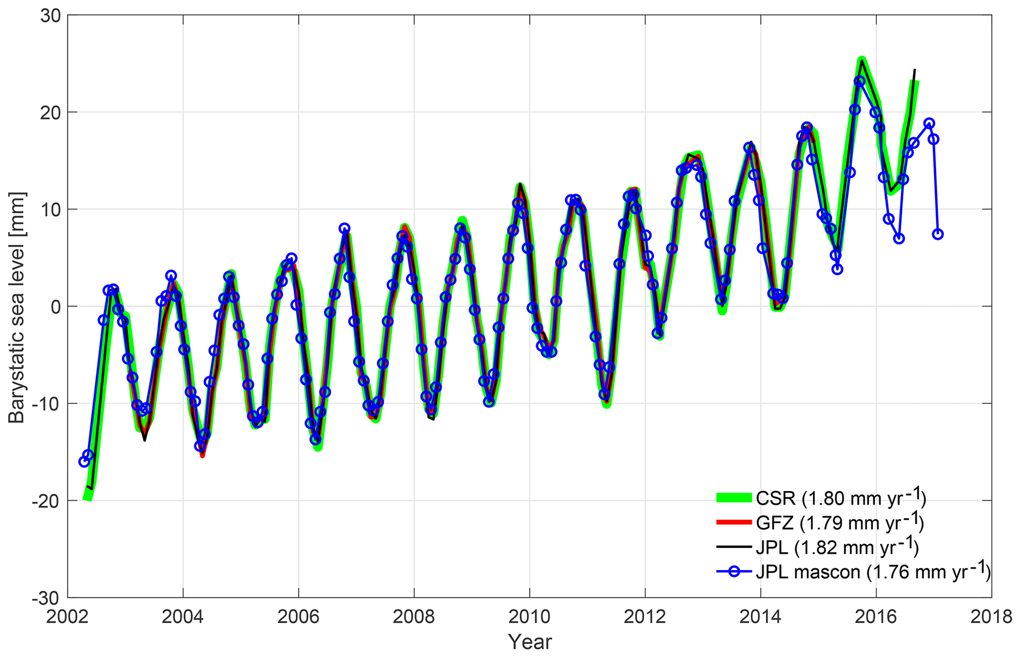
Figure 1Barystatic sea-level time series. Our estimates of trends and seasonal amplitudes for all three data centers are compared to JPL mascon solutions (Watkins et al., 2015). Results are plotted relative to the time means over the period January 2003 through December 2013. Trend values are provided for the period January 2005 through December 2015, except for GFZ solutions (January 2005 to December 2013), for a comparison to the sum of individual mass components (during January 2005 to December 2016) listed in Table 13 of the WCRP (2018) report: 1.65±0.23 mm yr⁻¹. As an additional point of comparison, Dieng et al. (2015) find GRACE-determined mass changes for the barystatic sea-level trend at 2.04±0.08 mm yr⁻¹ for January 2005–December 2013 from the mean of CSR, GFZ, and JPL Level-2 Release-05 spherical harmonic solutions.

Download

Monthly land water storage fields, $H(\mathit{\theta },\mathit{\varphi },t)$, may be generated by assembling the coefficients (Eq. 10) in an SH domain, as in Eq. (B1). Gaussian smoothing aimed at removing the data noise also attenuates the signals. An appropriate scaling of the fields is therefore essential. For the ice sheet and peripheral glaciers in Greenland, three non-overlapping sub-domains of Antarctica, and 15 regions of global glaciers and ice caps, we compare our estimates of average rate of regional mass change during February 2003 through June 2013 with those computed by Schrama et al. (2014) and derive the scaling factors – unique for CSR, GFZ, and JPL data products – for each of these 19 cryospheric domains. As for the non-cryospheric continental domains, Landerer and Swenson (2012) analyzed monthly land water storage signals obtained from the GRACE observations and the Noah land surface model, simulated within the Global Land Data Assimilation System (GLDAS-Noah), and derived global gridded gain factors. We combine these factors to scale $H(\mathit{\theta },\mathit{\varphi },t)$ for the entire continents. Our estimates of barystatic time series are comparable to, for example, JPL mascon solutions for both trends and seasonal amplitudes (Fig. 1).

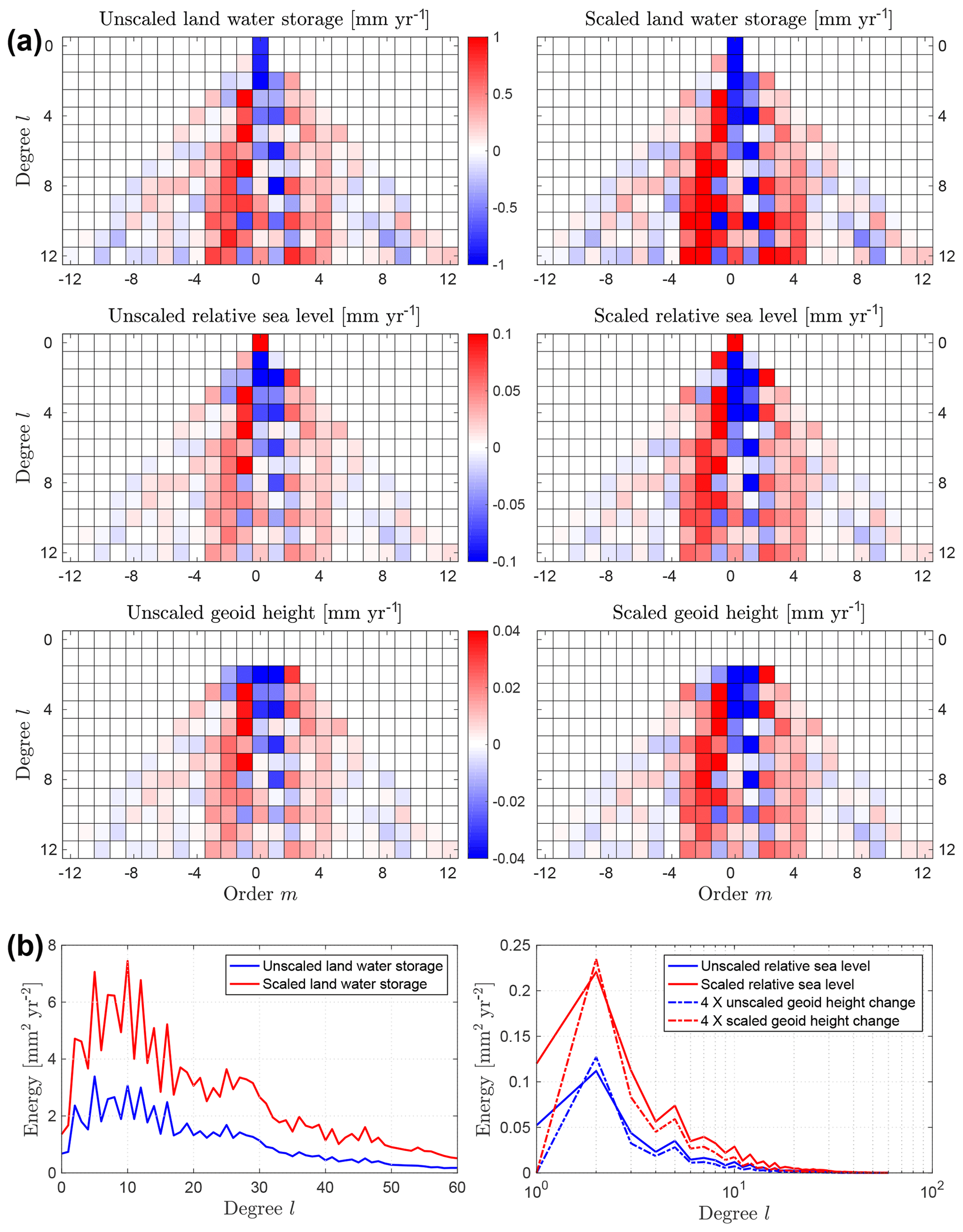
Figure 2Effects of scaling on the select spherical harmonic coefficients. (a) Scaling effects on the average rate of change in land water storage, relative sea level and geoid height, during April 2002 through March 2016. These solutions are based on JPL Stokes coefficients and are computed in the CM reference frame with the rotational feedback included. (b) Distribution of energy, computed for a given degree l as a sum of the squares of corresponding orders m, for unscaled and scaled solutions. Note the log scale on the x axis of the right panel. Unlike the geoid height change, the relative sea-level change has nonzero energy at l=0 with magnitudes of 1.16 and 2.37 mm² yr⁻² for unscaled and scaled solutions, respectively. Also note that solutions for geoid height change employ a different scale (factor of 4) for appropriate visualization.

Download

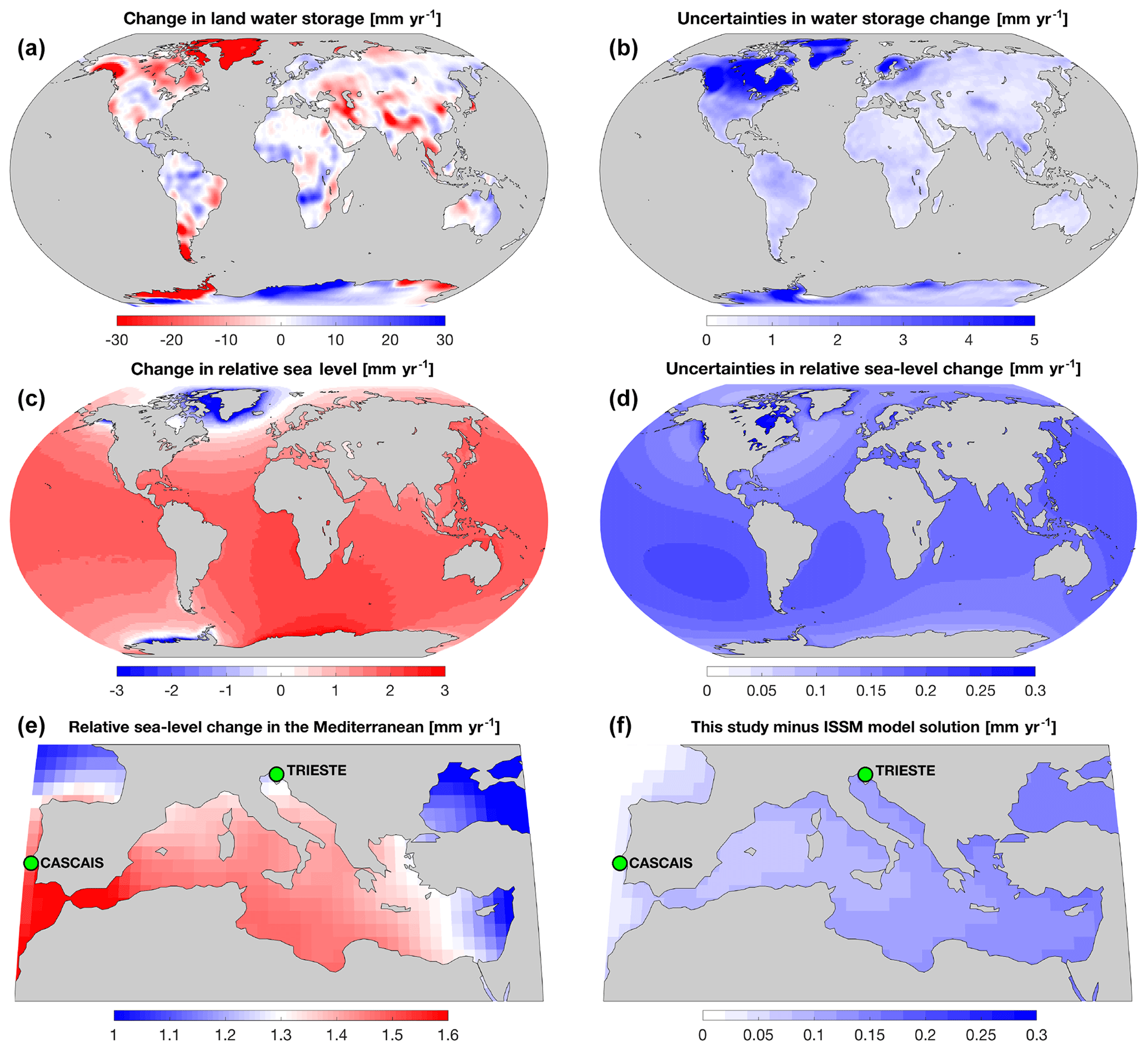
Figure 3Land load function, sea-level fingerprint, and uncertainties therein. Average rate of water equivalent height change in land water storage (a, b) and associated change in relative sea level (c, d) for the period April 2002 to March 2016 are shown with their corresponding 1σ uncertainties. Maps for sea-level fingerprint and uncertainty are produced by assembling the corresponding spherical harmonic coefficients provided with this article. These solutions are based on JPL Stokes coefficients and are computed in the CM reference frame with the rotational feedback included. A zoomed-in map of the Mediterranean Sea (e) is meant to highlight the local variability in sea-level fingerprint. The fingerprint-predicted trends for tide gauges at TRIESTE (1.26±0.18 mm yr⁻¹) and CASCAIS (1.50±0.17 mm yr⁻¹) reflect differences that are comparable to those associated with interdecadal atmospheric pressure trends (0.2±0.2 mm yr⁻¹) and the GIA-related fingerprint (≈0.2 mm yr⁻¹) (see Piecuch et al., 2016, and Stocchi and Spada, 2009, respectively). This illustrates one example of the importance of contemporary sea-level fingerprints for tide gauge data analysis and interpretation. Panel (f) is meant to show that our solutions are comparable to those obtained from a well-validated and higher-resolution ISSM sea-level solver (Adhikari et al., 2016); note that the solution discrepancy is within the 1σ uncertainties (compare with panel d).

Download

A detailed description of scaling may be found in Adhikari and Ivins (2016), who used the same recipe to post-process the CSR Release-05 GRACE Level-2 Stokes coefficients for robust reconstruction of interannual variability in position of Earth's spin axis. This gives us extraordinary confidence that the procedure for generating land water storage fields and corresponding fingerprints are not only sound but highly robust at long wavelengths. The effects of scaling on SH coefficients of select fields are shown in Fig. 2. Our model solutions are also robust. For example, our estimates of relative sea-level change (Fig. 3), vertical bedrock motion (not shown), and geoid height change (not shown) are consistent with the respective solutions computed using a well-validated sea-level solver (Adhikari et al., 2016) that operates on an unstructured global mesh of the Ice and Sea-level System Model (ISSM; https://issm.jpl.nasa.gov/, last access: 7 May 2019). We find that GFZ solutions are slightly different from CSR and JPL solutions (Fig. 4), although the difference in sea-level fingerprints is generally within 1σ uncertainties (compare Figs. 3d and 4d). We show the origin of discrepancies by plotting the degree variance spectrum.

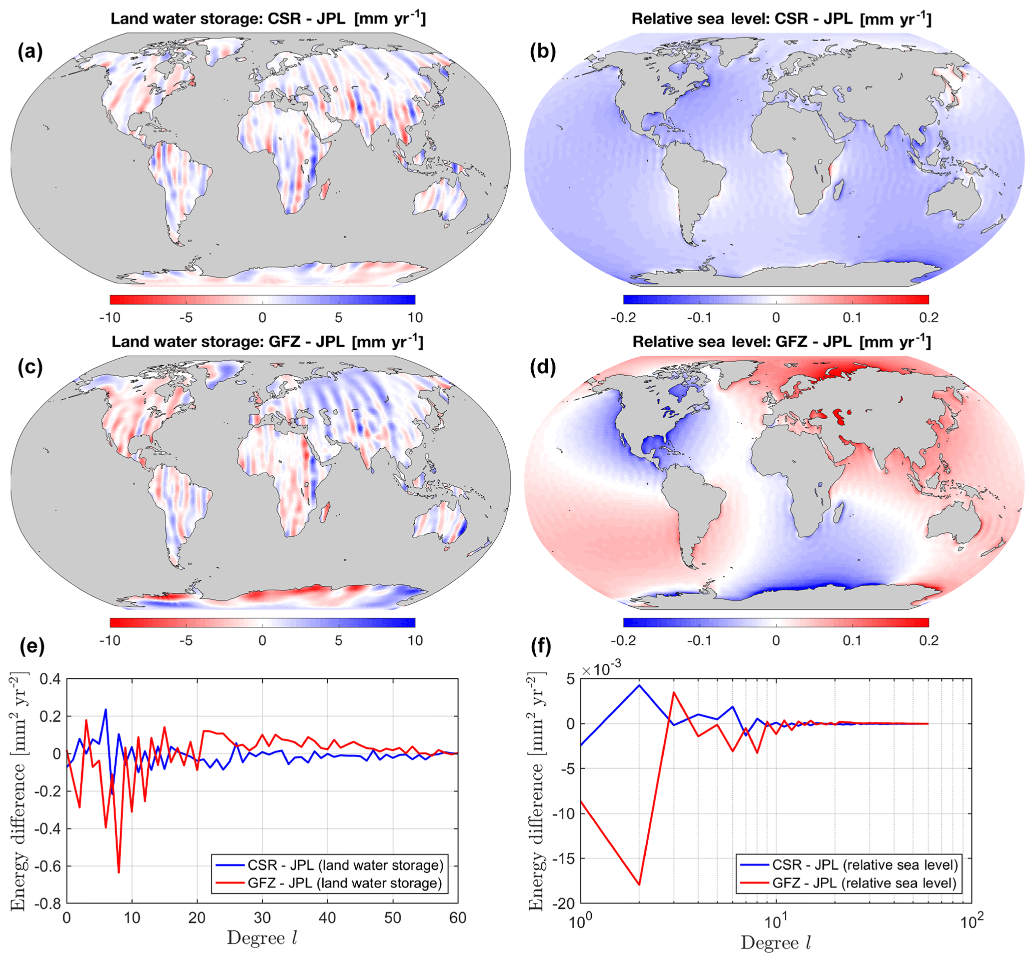
Figure 4Comparison of data centers for select fields. JPL solutions are subtracted from CSR and GFZ solutions for trend in land water storage change (a, c) and relative sea-level change (b, d) during January 2003–December 2013. The difference in the spectrum of energy distribution is also shown (e, f). Results are computed in the CM reference frame with the rotational feedback accounted for.

Download

Based on CSR, GFZ, and JPL Stokes coefficients, we provide with this article monthly SH coefficients of

• model forcing function, F_lm(t);

• geoid height change, [X_lm(t)+Y_lm(t)];

• vertical bedrock motion, $-\left[P_{lm}\left(t\right)+Q_{lm}\left(t\right)\right]$; and

• relative sea-level change, S_lm(t),

computed in both CM and CF reference frames with and without the rotational feedback included. Effects of Earth's rotation and the reference frame origin on select fields are shown in Fig. 5. The SH coefficients for sea-surface height may be obtained by summing coefficients for bedrock motion and those for relative sea-level change (see Eq. 1). While one may readily assemble these coefficients in an SH domain to retrieve the corresponding monthly fields, we also supply $\mathrm{0.5}{}^{\circ }\times \mathrm{0.5}{}^{\circ }$ gridded solutions for user convenience.

We provide uncertainty associated with monthly fields as well, both in terms of spatial maps and SH coefficients. Quantification of the uncertainty is determined by the following recipe. Based on the JPL Release-06 (GIA uncorrected) mascon solutions and associated standard errors (Watkins et al., 2015; Wiese et al., 2016), we use a Monte Carlo approach to generate 5000 ensemble members of monthly land water storage solutions. We apply a unique GIA correction, computed by Caron et al. (2018), to each of these ensemble members. Next we solve the sea-level equation to derive an equivalent number of solutions for $S(\mathit{\theta },\mathit{\varphi },t)$, $U(\mathit{\theta },\mathit{\varphi },t)$, and other fields. Finally, we quantify the standard errors associated with each field, weighted by the likelihood of each GIA model (Caron et al., 2018). Figure 3 shows our estimates of standard errors associated with the trends in land water storage and relative sea level.

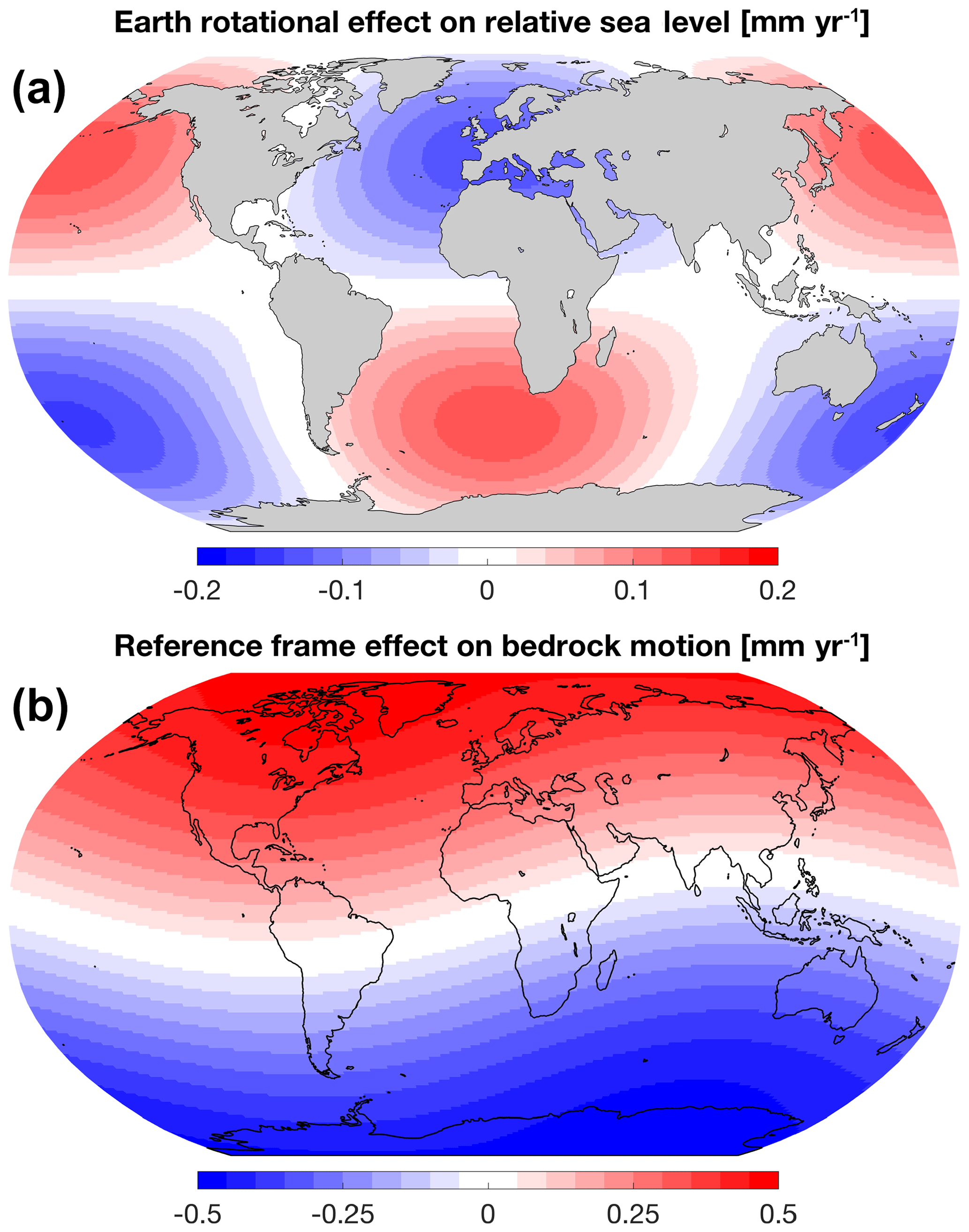
Figure 5Effects of (a) Earth's rotation and (b) reference frame on model solutions. Rotational feedback on the relative sea-level change exhibits a degree 2 spherical harmonic pattern and generally accounts for ≈10 % of the total signal (compare with Fig. 3c). Degree 1 load Love numbers depend on the choice of reference frame origin. The effect of reference frame – quantified here as the model solution computed in the CM frame minus the solution computed in the CF frame – is more pronounced in the vertical bedrock motion and the geoid height change (not shown). These results are based on JPL Stokes coefficients for the period April 2002 to March 2016.

Download

The utility of the data we provide is that they may be used to rigorously remove those patterns that are attributable to geoid height change and bedrock motions caused by on-land mass changes from ocean altimetry, bottom-pressure, and tide gauge studies. Such removal is essential for future studies of the patterns of sea-level change owing to internal variability of the climate system which drives changes in ocean density, fresh water fluxes, and circulation (e.g., Bilbao et al., 2015; Fasullo and Nerem, 2018).

As we supply sea-level fingerprints and complementary data products with and without rotational feedback, we owe the readers some additional words of caution and recommendations. First, from the Eulerian equations of rotational motion, we solve for the feedback consistently designed for periods longer than 434 d (the period of the Chandler wobble). The rationale is that both the solid Earth and ocean pole tide (Haubrich and Munk, 1959) are removed from the satellite solutions for GRACE gravimetry and TOPEX/Poseidon and Jason altimetry on a routine basis (e.g., Wahr, 1985; Desai, 2002; Desai and Yuan, 2006). The improvements in the ocean pole tide, in fact, have been accomplished by many years of assimilation of the altimetric mission data. Hence, at periods near, or less than, 434 d, the paths to unambiguously generating solutions to the sea-level equation with centrifugal potential and loading changes from the pole tide are unclear. We might assume that the relevant feedbacks are largely removed as a processing step in rendering Level 1-b and Level 2 GRACE data products. We keep, however, rotational feedback effects of an interannual nature in one set of monthly solutions, and another set of solutions lack these effects. The users of these data should understand the differences, as those employing approaches to using the data to evaluate altimetric time series of order 10 years in length will certainly be interested in using the rotational feedback version for the analysis of interannual trends and variability adjacent to Greenland, for example Müller et al. (2019), whereas users focusing on seasonal timescale fingerprints are recommended to employ those coefficients that lack the rotational feedback, as the altimetry and space gravimetry products employed likely have the sea-surface height and gravity effects of the annual polar motion, Chandler wobble, and associated pole tides removed.

It is also worthwhile to note that on timescales of decades the mantle primarily behaves elastically, perhaps with the exception at places where the tectonic history has brought heat, volatiles, and changes in mineral structure, such as water or reduced grain size, into the region, thus reducing the effective viscosity to values below about 5×10¹⁸ Pa s (e.g., Lange et al., 2014; Mitrovica et al., 2018; Nield et al., 2018). At such low values of viscosity in the upper mantle, stress relaxation can reduce both the effective influence of gravitational loading and the amplitude of fingerprints. While we acknowledge that this effect is quite difficult to quantify, it should be a second-order effect.

We presently store data in a public repository hosted by Harvard Dataverse (https://doi.org/10.7910/DVN/8UC8IR; Adhikari et al., 2019).

The first set of data we supply are SH coefficients of global field variables. The zip file “SLFsh_coefficients.zip” contains a total of 1780 data files: 133×4 for GFZ and 156×4 each for CSR and JPL. For the given data center, four files are provided for a particular GRACE month: with and without Earth's rotational feedback included while solving for sea-level fingerprints in both CM and CF reference frames. File names follow the GRACE naming convention. Solutions that correspond to the GSM file “GSM-2_2002095-2002120_GRAC_UTCSR_BA01_0600”, for example, are stored in four files named “SLF-2_2002095-2002120_GRAC_UTCSR_BA01_0600” under appropriate directories; we simply replace “GSM” by “SLF” to denote “sea-level fingerprints”. The time stamp (in YYYYDoY-YYYYDoY format) and the corresponding data center (five-character string containing CSR, GFZ, or JPL) also appear in the file name. The example file considered above contains sea-level fingerprint solutions for the period 95–120 d of year 2002 based on the Stokes coefficients provided by CSR. Header lines 5–7 in each file further clarify which data center the solutions correspond to, which reference frame is considered, and whether or not Earth's rotational feedback is accounted for. Each data file consists of a total of 18 columns: SH degree l, SH order m, and SH coefficients for model forcing function F_lm (four columns), relative sea level S_lm (four columns), geoid height change [X_lm+Y_lm] (four columns), and vertical bedrock motion $-[P_{lm}+Q_{lm}]$ (four columns). For each field, the first (last) two columns store cosine (sine) coefficients for our predicted mean and 1σ uncertainty, respectively. Users should note that the finite degree 0 order 0 harmonic in the monthly SLF files represents the finite mass changes for the global oceans.

The second set of data we supply are gridded maps of global field variables. We provide a total of 12 NetCDF files: four each for CSR, GFZ, and JPL. The file “SLFgrids_GFZOP_CF_WITHrotation.nc”, for example, stores solutions based on GFZ Stokes coefficients that are computed in the CF reference frame with the rotational feedback accounted for.

SA and ERI conceived the research and wrote the first draft of the paper. SA formulated the sea-level solver, with the help of ERI, and led the calculations, with the help of FWL (in estimating degree 1 Stokes coefficients) and TF and LC (in uncertainty quantification). All authors contributed to the analysis of the results and to the writing and editing of the paper.

The authors declare that they have no conflict of interest.

This research was supported by the JPL Research, Technology & Development Program (grant no. 01-STCR-R.17.235.118; 2017–2019) and the NASA Sea-Level Change Science Team (grant no. 16-SLCT16-0015; 2018–2020), as well as the NASA MEaSUREs program (grant no. 17-MEASURES-0031; 2019–2023).

This paper was edited by Giuseppe M. R. Manzella and reviewed by Don Chambers, Xuebin Zhang, and Makan A. Karegar.