the Creative Commons Attribution 4.0 License.
the Creative Commons Attribution 4.0 License.
 | 23 May 2019
Evolution of the ESA CCI Soil Moisture climate data records and their underlying merging methodology
Alexander Gruber
Tracy Scanlon
Robin van der Schalie
Wolfgang Wagner
Wouter Dorigo
The European Space Agency's Climate Change Initiative for Soil Moisture (ESA CCI SM) merging algorithm generates consistent quality-controlled long-term (1978–2018) climate data records for soil moisture, which serves thousands of scientists and data users worldwide. It harmonises and merges soil moisture retrievals from multiple satellites into (i) an active-microwave-based-only product, (ii) a passive-microwave-based-only product and (iii) a combined active–passive product, which are sampled to daily global images on a 0.25∘ regular grid. Since its first release in 2012 the algorithm has undergone substantial improvements which have so far not been thoroughly reported in the scientific literature. This paper fills this gap by reviewing and discussing the science behind the three major ESA CCI SM merging algorithms, versions 2 (https://doi.org/10.5285/3729b3fbbb434930bf65d82f9b00111c; Wagner et al., 2018), 3 (https://doi.org/10.5285/b810601740bd4848b0d7965e6d83d26c; Dorigo et al., 2018) and 4 (https://doi.org/10.5285/dce27a397eaf47e797050c220972ca0e; Dorigo et al., 2019), and provides an outlook on the expected improvements planned for the next algorithm, version 5.
Please read the corrigendum first before continuing.
-
Notice on corrigendum
The requested paper has a corresponding corrigendum published. Please read the corrigendum first before downloading the article.
-
Article
(5016 KB)
-
The requested paper has a corresponding corrigendum published. Please read the corrigendum first before downloading the article.
- Article
(5016 KB) - Corrigendum
- BibTeX
- EndNote


The European Space Agency's Climate Change Initiative for Soil Moisture (http://www.esa-soilmoisture-cci.org/, last access: 17 May 2019), hereafter referred to as ESA CCI SM, is dedicated to the development of consistent satellite-based long-term climate data records (CDRs) for soil moisture, aiming to serve climate science as well as numerous other communities (Dorigo et al., 2017). The first soil moisture CDRs produced by the ESA CCI SM were released in 2012. To date, the ESA CCI SM serves more than 6000 registered users, providing the basis for a host of scientific publications and data set applications (Dorigo et al., 2017).
Central to the ESA CCI SM is a merging algorithm, which, in essence, merges soil moisture retrievals from various satellites that have finite lifetimes and significantly different instrument characteristics (frequency, spatial resolution, temporal coverage, polarisation, revisit time, etc.) into three consistent multi-decadal data sets. This process faces innumerable scientific challenges and is therefore subject to continuous research and development. To date, seven product versions have been released to the general public. Differences between these product versions range from minor bug fixes and data set extensions to major structural changes in the way different satellite products are harmonised and merged. Recently, the European Commission's Copernicus Climate Change Service (C3S) started operational near-real-time CDR production, based on the algorithm developed within the ESA CCI SM.
While product improvements have been validated in numerous publications and the data set has been proven to be useful in a large number of applications (for a comprehensive review of these studies see Dorigo et al., 2015, 2017), none of the major scientific advances of the merging algorithm (since its first release in 2012; Liu et al., 2011, 2012; Wagner et al., 2012) have as yet been thoroughly documented in the scientific literature. This paper aims to fill this gap by providing a comprehensive and complete resource of the evolution of the ESA CCI SM merging algorithm up to the current version 4.4, which was released at the end of 2018. Moreover, an outlook on the expected developments that are planned for the next iteration, version 5, which is foreseen to be released in 2019, is provided.
The ESA CCI SM merging algorithm produces three individual products: (i) the ACTIVE product, which is generated by merging soil moisture retrievals from active-microwave-based sensors only, (ii) the PASSIVE product, which is generated by merging soil moisture retrievals from passive-microwave-based sensors only, and (iii) the COMBINED product, which is generated by merging soil moisture retrievals from both active-microwave-based and passive-microwave-based sensors. This paper reviews the three major ESA CCI SM merging algorithms which have been utilised in released versions to date:
-
The initial merging algorithm proposed by Liu et al. (2011, 2012), which has been used to generate all products up to version v02.2 (released early 2016; Wagner et al., 2018), is hereafter referred to as ESA CCI SM v2. This algorithm is a decision-tree-based approach that selects passive-microwave-based soil moisture retrievals, active-microwave-based soil moisture retrievals, or computes an arithmetic mean of the two based on their mutual correlation and vegetation optical depth.
-
The algorithm that has been used to generate the product versions v03.2 and v03.3 (released at the beginning and the end of 2017, respectively; Dorigo et al., 2018) and all Copernicus C3S CDR products up to version v201801 is hereafter referred to as ESA CCI SM v3. This algorithm is based on a statistically rigorous least squares merging approach.
-
The algorithm that has been used to generate product versions v04.2 and v04.4 (released at the beginning and the end of 2018, respectively; Dorigo et al., 2019) and is being used in the current Copernicus C3S CDR production system version (v201812) is hereafter referred to as ESA CCI SM v4. This algorithm uses an improved uncertainty characterisation approach to better parameterise the least squares merging scheme.
Note that the official version numbering system (vX.X) of the ESA CCI SM products follows the convention that the first (two-)digit number denotes the version of the underlying data merging methodology, while the second number marks releases with simple bug fixes and data set extensions.
Section 3 describes the level 2 (L2) soil moisture retrieval algorithms and the pre-processing steps of the individual input data sets, which are generally common to all ESA CCI SM product versions. Section 4 provides a review of the initial merging algorithm proposed by Liu et al. (2011, 2012) that was used in ESA CCI SM v2. Section 5 discusses the limitations of this decision-tree-based algorithm and the theoretical requirements for a statistically optimal merging scheme. Section 6 describes how such a statistical (least squares) merging scheme was implemented in ESA CCI SM v3 and Sect. 7 describes the improved uncertainty characterisation for this scheme that has been employed in ESA CCI SM v4. Section 8 demonstrates the performance evolution of the algorithm versions through comparison against ground reference data. Finally, Sect. 10 concludes with a discussion on the limitations and known issues with the current merging algorithm, which are currently under investigation and expected to contribute to the next version of the data set.
All ESA CCI SM algorithms to date merge pre-processed L2 data, that is, gridded soil moisture products retrieved from radiometrically calibrated backscatter or brightness temperature measurements. These data are resampled to a 0.25∘ regular grid using a Hamming-window approach and to daily time stamps (00:00 UTC) using a nearest-neighbour search. Note that tropical rainforest areas are masked out in all ESA CCI SM products because microwave satellite measurements do not contain any useful soil moisture signal in these regions due to signal scattering and attenuation of the vegetation (Ulaby et al., 2014).
Currently (at ESA CCI SM v4), soil moisture products from four active-microwave-based instruments (active products) and seven soil moisture products from passive-microwave-based instruments (passive products) are merged into the ESA CCI SM data sets. Sensors and missions, their temporal availability and their (most relevant) characteristics are summarised in Table 1.
Table 1Instrument characteristics for the products that are merged into the ESA CCI SM data sets (modified from Chung et al., 2018a).
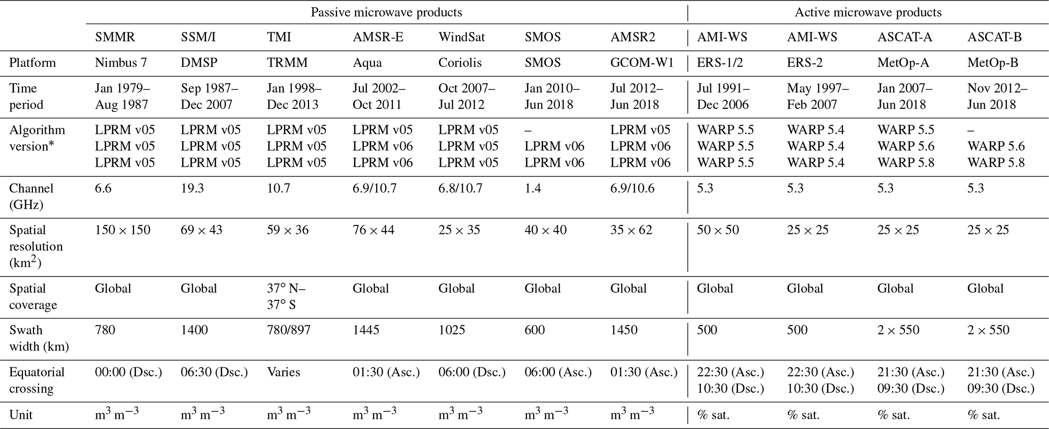
∗ L2 retrieval algorithm versions refer to those used for ESA CCI SM v2 (top), v3 (middle) and v4 (bottom). SMOS and ASCAT-B data were not included in ESA CCI SM v2.
3.1 Active products
Active products are retrieved using the TU Wien Water Retrieval Package (WARP) algorithm (Wagner et al., 1999; Naeimi et al., 2009), which is also used to generate the official operational ASCAT L2 soil moisture products for the Satellite Application Facility on Support to Operational Hydrology and Water Management of the European Organisation for the Exploitation of Meteorological Satellites (EUMETSAT H SAF, http://hsaf.meteoam.it/soil-moisture.php, last access: 17 May 2019). The WARP algorithm is a change detection approach that retrieves soil moisture as the degree of saturation by scaling azimuthally corrected radar backscatter measurements between the historically lowest and highest observed values (at each individual grid location), which are assumed to represent completely dry and saturated conditions, respectively. The multi-antenna multi-incidence angle capability of the ERS and ASCAT scatterometers are exploited to correct for the (seasonally varying) backscatter contribution of vegetation (Vreugdenhil et al., 2016). A threshold-based decision tree algorithm is applied to incidence angle normalised backscatter measurements to detect and remove measurements that were taken under frozen or freezing/thawing conditions where no reliable soil moisture retrieval is possible (Naeimi et al., 2012). For a complete description of the model and how it is applied to ERS and ASCAT data see the Algorithm Theoretical Baseline Document (ATBD) D2.1 Version 04.4 – Soil Moisture Retrievals from Active Microwave Sensors (Chung et al., 2018b). Information as to which WARP algorithm versions have been used for the different ESA CCI SM versions can be found in Table 1.
3.2 Passive products
Passive products are retrieved using the Land Parameter Retrieval Model (LPRM) algorithm (Owe et al., 2008). LPRM is a forward model which is based on the radiative transfer model of Mo et al. (1982) and distinguishes itself from other soil moisture retrieval algorithms due to its applicability to a wide range of frequencies (i.e. 1–20 GHz) and by using an analytical solution based on the Microwave Polarization Difference Index for the derivation of the vegetation optical depth (VOD; Meesters et al., 2005). For C-band and higher-frequency sensors, the data is filtered for frozen conditions using Ka-band-based temperature (Holmes et al., 2009) and for radio frequency interference (RFI; de Nijs et al., 2015; Li et al., 2004). For SMOS L-band retrievals, the filtering is based on the RFI and modelled (by the European Centre for Medium Range Weather Forecasts) temperature data are provided alongside the brightness temperature input data (SMOS L3TB). Soil moisture retrievals of all sensors are masked out if the VOD exceeds a certain threshold that depends on the microwave frequency of the respective sensor. For a complete description of LPRM and how it is applied see the Algorithm Theoretical Baseline Document (ATBD) D2.1 Version 04.4 – Soil Moisture Retrievals from Passive Microwave Sensors (de Jeu et al., 2018) as well as van der Schalie et al. (2016) and van der Schalie et al. (2017). Information as to which LPRM algorithm versions have been used for the different ESA CCI SM versions can be found in Table 1.
3.3 GLDAS Noah
GLDAS Noah (Rodell et al., 2004) is used as a scaling reference in the COMBINED product to obtain a consistent climatology throughout the entire ESA CCI SM period (Liu et al., 2011, 2012, see the next sections) and as an instrumental product for triple collocation analysis in the ACTIVE, PASSIVE and COMBINED products to obtain the L2 input data uncertainties (Su et al., 2014). More specifically, GLDAS Noah version 2.1 (and previously, GLDAS Noah version 1), which provides data from 2000 to the present, is used for both rescaling and triple collocation analysis (see the next sections). In earlier periods, GLDAS Noah version 2.0, which provides data from 1948 to 2010, is used for triple collocation analyses for L2 products where there is no temporal overlap with GLDAS Noah v2.1 (or v1). However, all L2 data sets are rescaled (for the COMBINED product) against GLDAS Noah v2.1 (previously, v1) due to inconsistencies with GLDAS Noah v2.0, which originate from the historic forcing data that were used in this version.
GLDAS Noah (all versions) provides 3-hourly estimates of soil moisture and other land variables for four different depth layers on a 0.25∘ regular grid. Top-layer (0–10 cm) soil moisture estimates at 00:00 UTC (coinciding with the resampled satellite input data) are used for rescaling and triple collocation analysis. Top-layer soil temperature (Ts) and snow water equivalent (SWE) estimates are used to mask out satellite measurements that were taken under conditions where no reliable soil moisture retrieval is possible (i.e. and SWE > 0 mm).
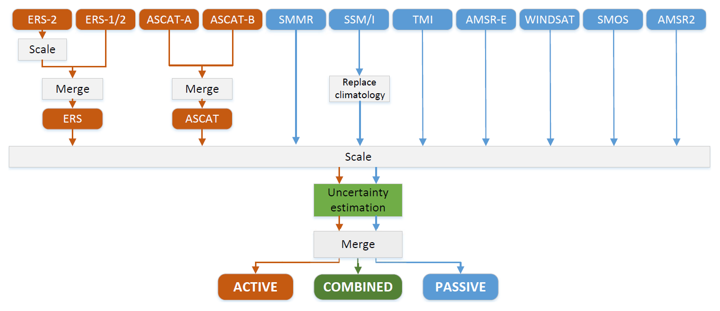
As previously mentioned, the merging algorithm for all product versions up to v2 (released early 2016; Wagner et al., 2018) remained relatively unchanged and is described in detail in Liu et al. (2011, 2012). Therefore, only its key features will be summarised here. The principal steps of the algorithm are illustrated in Fig. 1 and described in the following sections.
4.1 Harmonisation of L2 data
L2 input data sets from different missions are harmonised to a common climatology by matching the cumulative distribution function (CDF) of the individual data sets to that of a reference product, which was chosen to be the one that is expected to have the most stable climatology. For the active products this is ASCAT, as it is the direct successor instrument of ERS, with improved spatial resolution, temporal coverage and radiometric accuracy (Naeimi et al., 2009). For passive products it is AMSR-E due to its longer signal wavelength and higher spatial and temporal resolution (Liu et al., 2012). The CDF matching is realised by splitting the data sets into percentiles and rescaling these percentiles in a linear fashion (Liu et al., 2011).
For the harmonisation of the active products, a combined ERS-1/2 50 km (native) resolution time series is first simultaneously retrieved from well intercalibrated backscatter measurements from ERS-1 and ERS-2. Data gaps in these time series due to the on-board storage failure of ERS-2 in 2003 are filled with the experimental higher-resolution 25 km ERS-2-only soil moisture retrievals after rescaling (CDF matching) them against the combined ERS-1/2 data set. This complete ERS time series is then rescaled against ASCAT.
Passive products are harmonised as follows. WindSat and TMI retrievals are rescaled against AMSR-E, while AMSR2 is assumed to be properly intercalibrated with AMSR-E (which is most likely not always the case; see Parinussa et al., 2015 and Sect. 10). For SSM/I, only anomalies (calculated as deviations from the mean seasonal cycle) are rescaled against those of AMSR-E, while the mean seasonal cycle of SSM/I is fully replaced with that of AMSR-E due to its lack of consistency with other sensors (Liu et al., 2011, 2012). A merged SSM/I–TMI–AMSR-E time series is then created by selecting the best available sensor at a given time, assuming that the data quality negatively correlates with microwave frequency and the time since launch (Liu et al., 2012). Since TMI data are only available between ±37∘ latitude, SSM/I retrievals are used in the remaining latitude bands, even though they are considered to be less reliable than those from the longer-wavelength TMI sensor. Finally, SMMR observations are rescaled against the merged SSM/I–TMI–AMSR-E time series. Note that, as there is no temporal overlap between SMMR and successive sensors, this step scales the observations of different periods and thus assumes that there is no trend from the SMMR period (1978–1987) to the combined TMI–SSM/I–AMSR-E period (1987–2011) (Liu et al., 2012).
4.2 Generation of the ACTIVE and the PASSIVE product
The ESA CCI SM v2 ACTIVE product is generated by concatenating ASCAT and the rescaled combined ERS time series. Since this product is provided in the ASCAT data space, i.e. as the degree of saturation, a porosity map derived from the Harmonized World Soil Database (HWSD; Nachtergaele and Batjes, 2012) is provided alongside the data in order to allow the soil moisture estimates to be converted to volumetric units if required.
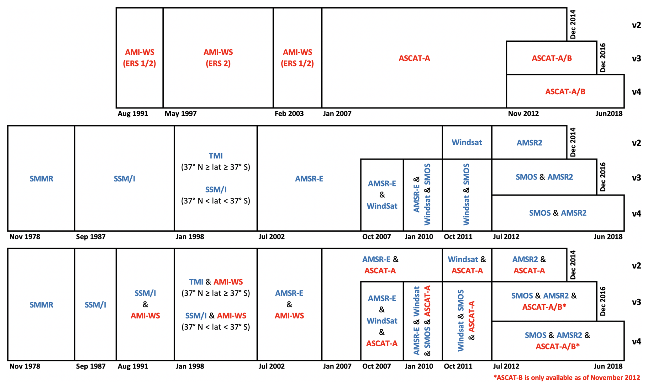
Figure 2Merging periods and sensor selection of the ACTIVE (top), PASSIVE (middle) and COMBINED (bottom) ESA CCI SM v2, v3 and v4 products.
The ESA CCI SM v2 PASSIVE product is generated by concatenating the rescaled SMMR data set, the harmonised and pre-concatenated AMSR-E–TMI–SSM/I time series and AMSR2. Note that in the ESA CCI SM v2 ACTIVE and PASSIVE products, measurements from different sensors are not merged. At all time steps, the presumed best-performing sensor operational at that date is selected, disregarding potentially available observations from the other sensors. Figure 2 illustrates the resulting sensor selection per time and latitude.
4.3 Harmonisation of the ACTIVE and the PASSIVE product
The ACTIVE and the PASSIVE products are harmonised by rescaling them against GLDAS Noah soil moisture simulations. The rationale for using a land surface model as a scaling reference for harmonisation is its supposedly long-term consistent climatology. For more details on the implications and caveats of this choice see Liu et al. (2011, 2012) and Sect. 10.
4.4 Generation of the COMBINED product
The harmonised ACTIVE and PASSIVE data sets are merged into the COMBINED product by following a decision tree that selects either one of the products alone or uses the arithmetic mean of both during a particular period based on the assumption that active retrievals tend to perform better in more densely vegetated areas, whereas passive retrievals tend to perform better in more sparsely vegetated areas (Liu et al., 2011, 2012). For each merging period (see Fig. 2) and at each quarter degree grid cell, the Pearson correlation coefficient between the ACTIVE and the PASSIVE product is calculated. At all locations and during each period where the correlation exceeds 0.65, the arithmetic mean between the ACTIVE and the PASSIVE product is used at time steps where both are available. If one data set does not provide a valid observation at a particular time step (due to L2 quality control and orbit characteristics), the observation of the respective other data set is used. At locations and in periods where the correlation threshold is not met, the ACTIVE data set is selected if the multi-year average AMSR-E-based VOD at that location is above a certain threshold and the PASSIVE data set is selected if the VOD is below that threshold. The threshold is taken as the average of multi-year average AMSR-E-based VOD estimates over all regions where the correlation between the ACTIVE and the PASSIVE products does exceed the aforementioned correlation threshold of 0.65 (i.e. where the ACTIVE and the PASSIVE product are expected to be of comparable quality). In regions and periods where ERS data are scarce due to the failure of the on-board storage (resulting in a temporal coverage below 15 %), passive observations are used to fill these gaps, even if the correlation and VOD threshold suggest the use of the ACTIVE product only.
In summary, the merging algorithm behind ESA CCI SM v2 COMBINED product is a ternary decision scheme that selects either active-microwave-based retrievals alone, passive-microwave-based retrievals alone or an unweighted average of the two based on their mutual correlation and average VOD conditions at a particular time and location.
While the ternary ESA CCI SM v2 decision tree algorithm described above has proven itself to be a robust way of merging soil moisture products from various satellites (Dorigo et al., 2015), it will hardly ever provide estimates that are optimal in a statistical sense. As known from (generalized) least squares, deriving the best linear unbiased estimator for a measurand from different simultaneous measurements of that measurand with supposedly different qualities requires rigorous consideration of their individual errors and error correlations (Aitkin, 1935). Specifically, such an optimal estimate would be the weighted average of the individual measurements with the weights being derived from their error variances and covariances (Gelb, 1974). To understand this, consider an arbitrary number N of simultaneous measurements of the measurand y, contained in the measurement vector x:
The (N×2) design matrix A represents zero- and first-order (additive and multiplicative) systematic errors in x and the column vector ε represents independent (from y) additive Gaussian random errors in x. The measurand vector y=(1 y)⊺ allows for the consideration of additive systematic errors. Note that Eq. (1) could be easily extended with higher-order systematic errors by extending the column dimension of the design matrix and the row dimension of the measurand vector but not with different types of random errors as the method of least squares per definition allows for independent additive Gaussian noise only. In any case, Eq. (1) is the most commonly used error model for soil moisture data sets (Gruber et al., 2016b). The least squares solution, that is, the minimum random error variance estimate for y, is given as follows:
where the weight matrix is the inverse of the error covariance matrix with diagonal elements that are the error variances of the measurements ( with i∈x) and off-diagonal elements that are their error covariances ( with and i≠j).
In practice, the success of Eq. (2) depends on the degree to which systematic errors and the error covariance matrix (i.e. A and C) can be accurately estimated. Note, however, that, even if only relative systematic differences between the measurements are known, Eq. (2) still provides a minimum random error variance estimate (up to the remaining unknown systematic component). Recently, Gruber et al. (2017) proposed an implementation of Eq. (2) for merging active and passive microwave soil moisture retrievals, which utilises triple collocation analysis (TCA; Stoffelen, 1998; Gruber et al., 2016b) to estimate the input data uncertainties (i.e. diagonal elements of C) and CDF matching for a priori correction of relative systematic differences. This merging scheme formed the basis for the ESA CCI SM v3 product.
Gruber et al. (2017) showed that for a combination of ASCAT and AMSR-E retrievals a least squares merging scheme approach based on TCA outperforms the ternary merging scheme of ESA CCI SM v2. In the following sections we discuss how the scheme was implemented and adapted for merging four active and seven passive input data sets into the ACTIVE, the PASSIVE and the COMBINED ESA CCI SM v3 products (Dorigo et al., 2018). The principal steps are illustrated in Fig. 3. Note that the ESA CCI SM v3 algorithm continues to employ a two-stage merging scheme. That is, all active and passive data sets are first merged into the ACTIVE and the PASSIVE product, respectively, which are then further merged into the COMBINED product.
6.1 Harmonisation of L2 data
The input data harmonisation is largely identical to that in ESA CCI SM v2 (see Sect. 4.1). ASCAT observations from MetOp-B, which were additionally included in v3, are treated as perfectly intercalibrated with those from MetOp-A and arithmetically averaged on days and at locations where both satellites provide collocated measurements. SMOS, which was additionally included in v3, is, as all the other products, rescaled (CDF matched) against AMSR-E.
6.2 Uncertainty estimation for (harmonised) L2 data
Following Gruber et al. (2017), estimates of the random error variances (i.e. uncertainties) of the L2 data sets, required for the parameterisation of the employed least squares merging scheme, are obtained through TCA. TCA simultaneously estimates uncertainties in three spatially and temporally collocated data sets with errors that are required to be mutually uncorrelated. This requirement is commonly assumed to be met when applying TCA to one active-microwave-based, one passive-microwave-based and one land surface model-based soil moisture data set (Scipal et al., 2008; Gruber et al., 2016b). Accordingly, uncertainties in all active and passive products (except for SMMR, which does not temporally overlap with any of the active data sets) are estimated as follows:
where the subscripts refer to the active (a), the passive (p) and the land surface model (m) time series; is the temporal variance of data set i; and σi,j is the temporal covariance between data sets i and j with . Uncertainty estimates for each active (passive) data set are obtained by applying Eq. (3) to that data set in combination with the respective passive (active) data set with the longest temporal overlap and GLDAS Noah.
Note that the represent temporal mean data set uncertainties. Consequently, weights derived thereof (i.e. the P matrix in Eq. 2) are average weights for the period for which TCA was applied, although actual retrieval uncertainties (of individual sensors) may change over time (see Sect. 10). For more details on TCA we refer to Gruber et al. (2016b). Note also that, while errors of active and passive products are commonly assumed to be uncorrelated, significant correlations between the errors of different passive products may occur. Therefore, merging them into the PASSIVE product would require estimates of these error correlations in order to properly parameterise the full error covariance matrix in Eq. (2). Gruber et al. (2016a) proposed a modification of TCA which potentially allows the estimation of such error correlations, but this method has not yet been validated on a global scale and was found to be particularly susceptible to small sample sizes (sample sizes of products that are merged into the PASSIVE product are considered small in this context). Hence, lacking the ability to robustly estimate them, off-diagonal elements in the error covariance matrix are neglected in ESA CCI SM v3. The consequences of doing so are discussed in the next section and in Sect. 10.
6.3 Generation of the ACTIVE and the PASSIVE product
As in ESA CCI SM v2, the ACTIVE product is generated by concatenating the harmonised ERS and ASCAT time series because they do not have temporally overlapping observations which would allow for statistical merging. Consequently, their uncertainties, estimated from TCA, are merely appended to the product as auxiliary information and not used in the merging scheme.
Passive data sets are merged into the PASSIVE product as follows. Before October 2007 (i.e. before the launch of Coriolis, carrying WindSat), the low temporal coverage of the available sensors was assumed to render TCA-based error variance estimates too uncertain for a robust derivation of relative merging weights due to the susceptibility of TCA to small sample sizes (Zwieback et al., 2012). Consequently, SMMR, SSM/I, TMI and AMSR-E observations before October 2007 are concatenated in the same way as in ESA CCI SM v2, that is, by selecting the best available sensor at a particular time and location (see Fig. 2). Note that this was a relatively ad hoc albeit conservative assumption which has not yet been tested thoroughly but will be for future product versions (see Sect. 10).
All sensors available after this period (i.e. AMSR-E, WindSat, SMOS and AMSR2) are merged by employing the least squares estimator in Eq. (2) in the following manner: since the data sets are already harmonised, i.e. rescaled to a common climatology, the design matrix A is taken to be a column vector with all values being one. The error covariance matrices C required to calculate P (i.e. the relative weights for averaging the data sets) are constructed for each grid cell and for each merging period from the TCA-based uncertainty estimates of all sensors that are available during that particular period (see Fig. 2). As mentioned above, error cross-correlations are neglected. That is, off-diagonal elements in C are held zero, which may lead to biases in the estimated weights in case the errors of different passive data sets are significantly correlated (see Sect. 10). However, while this may reduce the efficiency (in uncertainty reduction) of the least squares estimator in several cases, it cannot lead to a substantial uncertainty increase (with respect to the individual L2 input products) because error correlations only pull the weights further towards the best product. If neglected, better products are still attributed with higher weights.
Note that the different sensors do not provide valid retrievals at every time step due to their orbit geometry and the L2 quality control (see Sect. 3). Consequently, if, during a particular merging period (see Fig. 2), a data set with significantly larger uncertainties has a higher temporal measurement coverage than the others, simply merging all available observations at each time step might result in a significantly larger overall uncertainty (of the merged time series) than that of the lower-uncertainty input time series alone. Therefore, to provide a trade-off between the best possible temporal measurement density and the lowest possible (average) uncertainty in merged time series, ESA CCI SM v3 imposes a minimum threshold for the cumulative weight of valid measurements available on a particular date, which has to exceed 1∕2N where N is the number of sensors in orbit and operational during that merging period. If this threshold is not met, no soil moisture estimate is provided for that day. For example, assume that for merging AMSR-E, WindSat and SMOS into the PASSIVE product, their weights as derived from their relative SNR at a particular location are 0.1, 0.05 and 0.85, respectively. Because N=3, the minimum-cumulative-weight threshold is 0.17. Therefore, if, on a particular day, only AMSR-E and WindSat observations are available, which have a cumulative weight of 0.15, no soil moisture estimate is provided. For more details on the choice and the implications of this threshold see Gruber et al. (2017).
6.4 Harmonisation of the ACTIVE and the PASSIVE product
As was the case with ESA CCI SM v2, in ESA CCI SM v3, before merging the ACTIVE and the PASSIVE products, their climatologies are harmonised by rescaling them against GLDAS Noah soil moisture simulations.
6.5 Uncertainty estimation for the (harmonised) ACTIVE and PASSIVE products
As mentioned in Sect. 6.2, TCA estimates represent the average retrieval uncertainties during the period in which TCA was applied. Since the uncertainties in the ACTIVE and PASSIVE products change significantly depending on which input data sets are used or merged at a particular point in time, uncertainties are estimated (from Eq. 3) separately for all periods with different sensor availabilities (see Fig. 2). In addition to TCA-based uncertainty estimates, significance levels (p values) of the Pearson correlation between the ACTIVE data set, the PASSIVE data set and GLDAS Noah are calculated (separately for the same periods) in order to screen for unreliable TCA estimates (see the next section).
6.6 Generation of the COMBINED product
TCA estimates of soil moisture uncertainty are known to have limited reliability in certain regions such as deserts, high latitudes or areas with dense vegetation (Dorigo et al., 2010; Al-Yaari et al., 2014). Using these estimates to parameterise the covariance matrix in Eq. (2) could thus significantly alter the integrity of the least squares estimator. Therefore, following the approach of Gruber et al. (2017), p values are used to verify the reliability of TCA estimates and to fall back on the use of either active or passive retrievals alone, an unweighted average of the two, or to completely mask the grid cell during that period if uncertainty estimates and/or soil moisture retrievals are deemed unreliable. Specifically, the decision of whether to use the ACTIVE product alone, the PASSIVE product alone, an unweighted average of the two, the least squares estimate or to disregard the grid cell completely is based on the relative p value. combination as illustrated in Table 2. If the least squares estimator is used, a minimum-weight threshold of 0.25 (1∕2N where N=2, i.e. ACTIVE and PASSIVE) is again imposed on dates where only one of the data sets (ACTIVE or PASSIVE) provides a valid observation (see Sect. 6.3). More details and an evaluation of this classification scheme is provided in Gruber et al. (2017).
Table 2Merging scheme based on the one-tailed p value for the correlation between active (a), passive (p) and modelled (m) soil moisture with a 0.05 significance level (modified from Gruber et al., 2017).

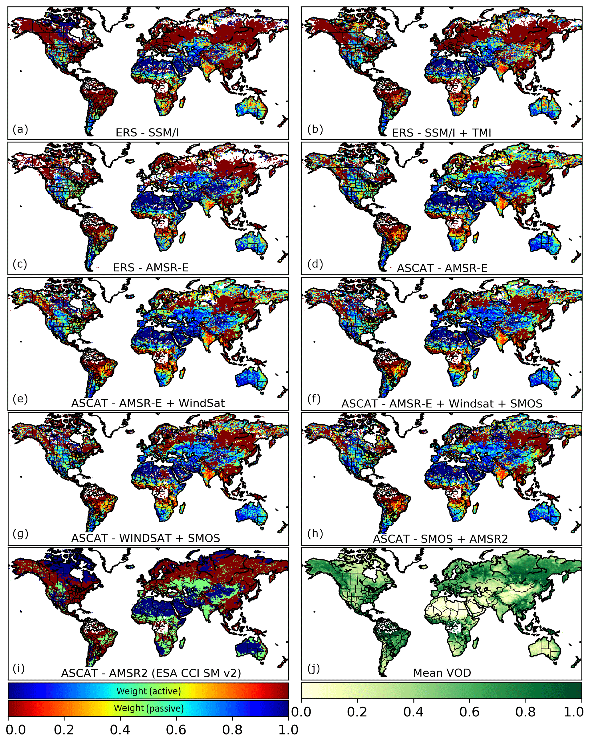
Figure 4Weights for merging the ACTIVE and PASSIVE products in the ESA CCI SM v3 algorithm (all sensor periods, a–h), weights for merging the ACTIVE and PASSIVE products in the ESA CCI SM v2 algorithm (latest period, i) and average VOD derived from AMSR-E (j).
Figure 4 shows the relative weights during each merging period (see Fig. 2) which are used for merging the ESA CCI SM v3 ACTIVE and PASSIVE products based on the TCA uncertainty estimates and the p-value mask. As a reference, the weight distributions amongst the ACTIVE and PASSIVE product in the ESA CCI SM v2 algorithm (only during the last merging period) and average VOD conditions at each location are given. The main apparent feature is that weight distributions in all merging periods largely follow VOD patterns. While the ESA CCI SM v2 algorithm was specifically designed to do so, the fact that the uncertainty-based weights in the ESA CCI SM v3 algorithm do this as well (with a much better resolution) strengthens the evidence for the assumption that active products tend to perform better in more densely vegetated areas, whereas passive products tend to perform better in more sparsely vegetated regions. This behaviour forms the basis for the improved weight derivation in the ESA CCI SM v4 algorithm for regions where TCA estimates are deemed unreliable, which is discussed in the following section.
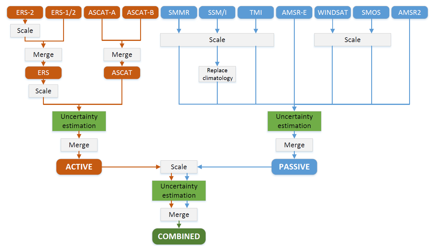
Algorithmic changes which were implemented for generating the ESA CCI SM v4 products (Dorigo et al., 2019) tackled two specific issues with the way in which the uncertainty estimates for the least squares merging are obtained in ESA CCI SM v3. First, the two-stage merging approach caused biases in the relative weights that are attributed to the ACTIVE and PASSIVE products during the different merging periods (see Fig. 2). These biases resulted from the irregular temporal measurement availability of the individual L2 input data sets, which led to temporal uncertainty variations in the PASSIVE product during the different merging periods depending on which sensors have valid observations and are merged together on a particular day. Such uncertainty variations cannot be accurately captured by the single uncertainty estimates used to merge the ACTIVE and PASSIVE products together. Second, even though seemingly robust, the p-value-based ternary decision in areas where TCA estimates are deemed unreliable also resulted in biased (with respect to statistically optimal) weight estimates very similar to the biases in the ESA CCI SM v2 algorithm because it selects weights of 0, 0.5, or 1 irrespective of the actual data set uncertainties (see Sect. 5). The following sections will describe the changes that have been implemented to address these issues. The resulting modified ESA CCI SM v4 algorithm is illustrated in Fig. 5.
7.1 Direct merging of L2 observations into the COMBINED product
In ESA CCI SM v4, the COMBINED product is generated by directly merging L2 input data sets instead of the previously merged ACTIVE and PASSIVE products (as is the case in ESA CCI SM v2 and v3). This allows the estimation of temporally dynamic relative merging weights for each individual sensor based on which sensors provide valid observations on a particular day. For this purpose, all L2 input data sets are first directly scaled against GLDAS Noah to harmonise their climatology (as for the earlier versions, the SSM/I climatology is first replaced with that of AMSR-E). Uncertainties are then estimated (see below) for each individual product and used to construct error covariance matrices for all merging periods depending on the sensor availability during these periods (see Fig. 2). Finally, the data sets are merged into the COMBINED product, again using the minimum-weight threshold of 1∕2N on dates where not all input products available in that merging period provide valid measurements (see Sect. 6.3).
7.2 VOD-based uncertainty estimation
As was shown in Fig. 4, uncertainty estimates and hence merging weights largely follow VOD patterns. To obtain uncertainty estimates in regions where TCA estimates are not trusted, i.e. where not all three data sets used in TCA are significantly correlated, an empirical polynomial regression approach that predicts uncertainties from average VOD conditions at a particular location was introduced. Specifically, a polynomial function is fitted between mean VOD (estimated from AMSR-E C-band observations between 2002 and 2011) and TCA-based signal-to-noise ratio (SNR) estimates using VOD and SNR tuples from all grid cells where TCA estimates are assumed to be reliable, i.e. where all three data sets are significantly (p<0.05) correlated (see Fig. 6). Regression coefficients are calculated separately for each L2 input product and used to predict their SNR levels () from the mean VOD at grid cells (i) where the SNR could not be estimated from TCA:
where aj are the polynomial coefficients and k is the degree of the polynomial function. k was chosen to be 3 for TMI and WindSat and 2 for all other sensors, which was empirically found to provide the best fit for the regression. Notice that regression coefficients are fitted between VOD and SNRs and not between VOD and uncertainties directly in order to account for varying signal variance across the grid cells that is used for the regression (Gruber et al., 2016b). SNRs are then converted into uncertainties as follows:
The overshooting in the regression curve of TMI for high-VOD values does not impact the final data product as grid cells with such high-VOD values are masked out by the L2 quality control process. The overshooting of WindSat for low VOD values affects a few grid cells in very dry regions and cannot be avoided by changing the polynomial order, as this would lead to overshooting in the more relevant VOD regions. SNR values at different grid cells and for particular VOD ranges sometimes show a significant variability around the corresponding estimate of the regression, which directly translates to uncertainties in the weight estimates that are used for the least squares merging. However, these uncertainties are assumed to be, on average, lower than the bias introduced by the p-value-based ternary decision of a weight of either 0, 0.5 or 1 as adopted in ESA CCI SM v2 and v3.
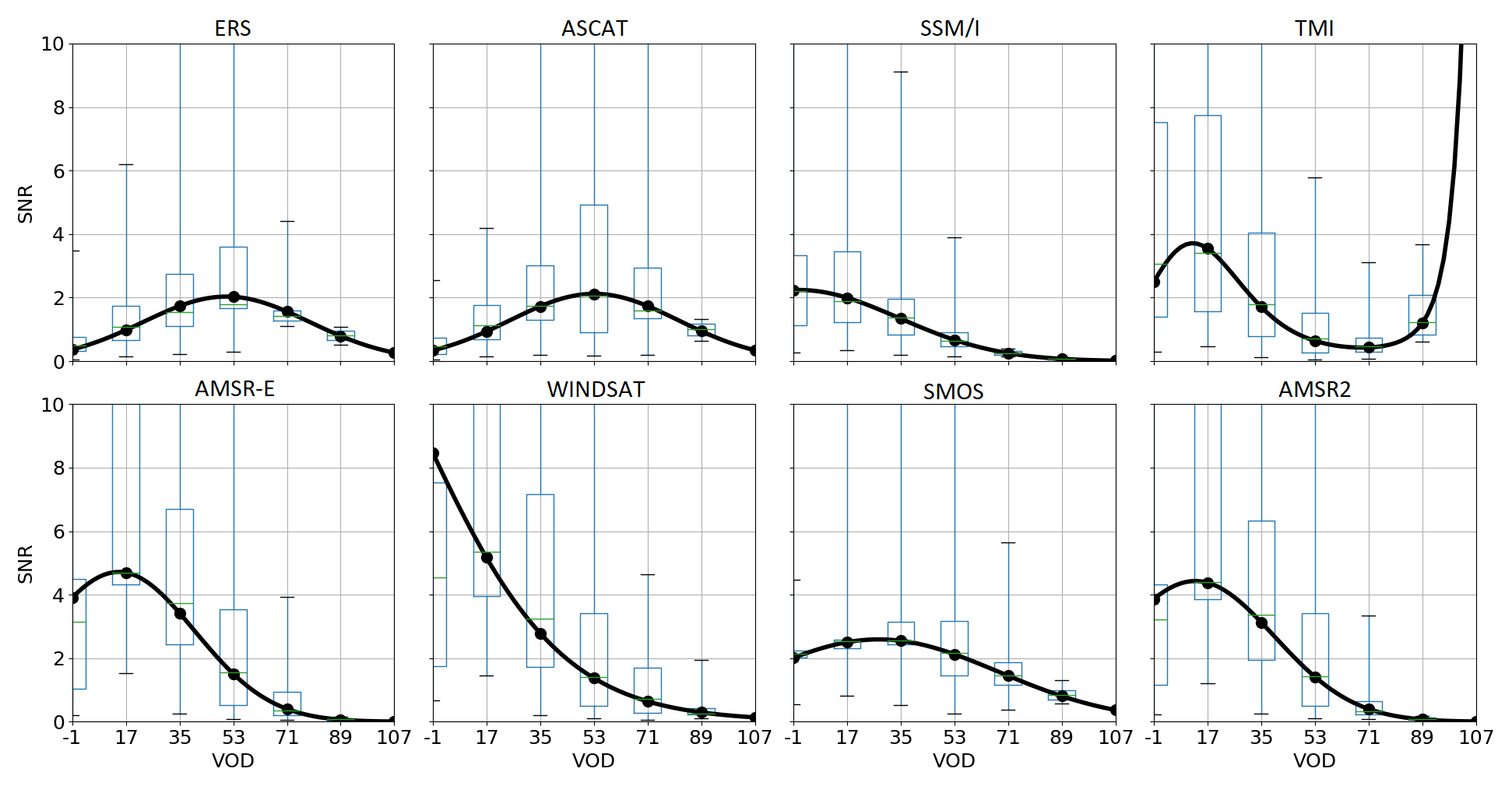
Figure 6Regression functions between VOD and SNRs (in decibel units) of all L2 products. Box plots show the median, the interquartile range and the 5 and 95 percentiles, respectively.
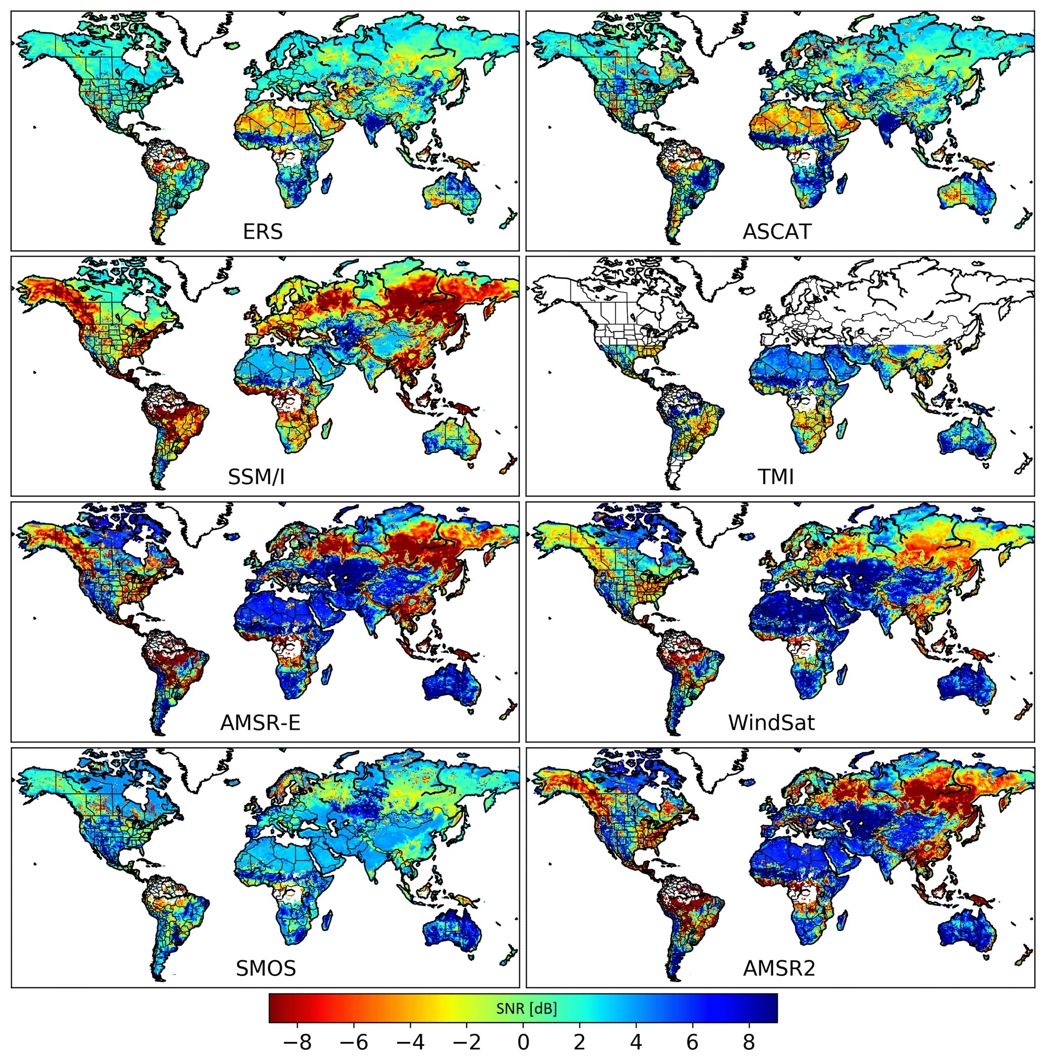
Figure 7SNR (in decibel units) of all L2 input products with uncertainties estimated from TCA and the VOD regression.
Figure 7 shows the combined TCA and VOD regression-based global SNR maps which are ultimately used to derive the merging weights for Eq. (2). Patterns generally follow common understanding. SNRs of active sensors are higher in more densely vegetated regions, whereas SNRs of passive sensors are higher in more sparsely vegetated areas (Dorigo et al., 2010; Liu et al., 2011, 2012; van der Schalie et al., 2018). SNRs of passive sensors largely depend on the microwave frequency (Liu et al., 2012; Parinussa et al., 2011, 2012). AMSR-E and AMSR2 (both C-band) SNRs are largely comparable and, in general, are higher than those for the higher-frequency (Ku-band) of SSM/I. SMOS (L-band) SNRs are, on average, relatively high and show a lower spatial variability as their longer wavelength makes the observations less sensitive to variation in vegetation.
Note that, as is the case in ESA CCI SM v3, SSM/I and TMI retrievals are never merged together or merged with AMSR-E, i.e. SSM/I data are only used at high latitudes where TMI data are not available, and neither of the two is used after AMSR-E becomes available (see Sect. 6.3). Nevertheless, their uncertainties are in many areas comparable with each other and with those of the other sensors, suggesting that they might add valuable information when included in the least squares merging scheme, which will be considered for future product versions (see Sect. 10).
7.3 P-value-based quality control
In ESA CCI SM v4, for the generation of both the PASSIVE and the COMBINED product, correlation significance levels are used to completely mask out individual L2 input products that are deemed unreliable at a particular location and during a particular merging period (in cases where more than one product is available for merging). For this purpose, the p-value mask that is used in the ESA CCI SM v3 product (see Sect. 6.6) was modified as shown in Table 3. All measurements from the target satellite product that is being tested for reliability are masked out if they do not correlate significantly with both soil moisture estimates from GLDAS Noah and the measurements from the second satellite product used for TCA, or if they correlate significantly with the reference satellite product but not with the model time series.
Table 3Merging scheme based on the one-tailed p value for the correlation between the model (m), the reference satellite (r), the target satellite (t) and soil moisture with a 0.05 significance level.

The rationale behind the latter is that potential non-zero error correlations, arising, for example, from uncorrected vegetation variations (Zwieback et al., 2018), may lead to spurious correlations between the two products, even though they do not contain useful soil moisture information. Note, however, that the decisions in the p-value mask were empirically tuned to lead to a good performance (of the merged products) in terms of correlation against the ERA-Land soil moisture product. Consequently, decisions that are based on significance levels of the correlation against GLDAS Noah may be questionable, since the two models are most likely not fully independent. This issue is currently under investigation and will be addressed in future product versions (see Sect. 10).
The previous sections provided a methodological review of the merging algorithm behind the ESA CCI SM (and Copernicus C3S) products. Even though this is not a validation paper, this section shall provide an overview of the performance evolution of the presented product versions, i.e. ESA CCI SM v2, v3 and v4. To this end, both absolute and anomaly time series (calculated by removing seasonal dynamics which are estimated by applying a 35-day moving average window) of the ACTIVE, PASSIVE and COMBINED data sets from the latest public release of each product version (i.e. v02.2, v03.3 and v04.4) are correlated against globally distributed in situ soil moisture observations from the International Soil Moisture Network (ISMN; Dorigo et al., 2011a, b). Only in situ measurements that are flagged “good” by the ISMN internal quality control (Dorigo et al., 2013) are used for the comparison. Unreliable ESA CCI SM soil moisture estimates are masked out as described in the previous sections. Products are evaluated from October 2007 onwards as significant improvements are mainly expected after this date due to the use of multiple passive satellites within the merging scheme (see Sect. 6) and the improved temporal data coverage of both the ESA CCI SM products and the ISMN stations available for validation.
The majority of the ISMN stations are distributed over large areas and most ESA CCI SM grid cells contain only a single measuring station. Direct comparisons (i.e. relative correlation coefficients) are therefore affected by significant upscaling errors (in addition to in situ sensor measurement errors; Miralles et al., 2010; Gruber et al., 2013). TCA potentially allows this influence to be avoided by directly estimating correlation coefficients with respect to the unknown “true” soil moisture signal (McColl et al., 2014). Chen et al. (2017) showed that these TCA-based correlation coefficients are independent of in situ sensor and representativeness errors. However, TCA requires the errors of the data sets to which it is applied to be mutually independent. Usually, any combination of in situ soil moisture measurements, active-microwave-based soil moisture retrievals, passive-microwave-based soil moisture retrievals and modelled soil moisture estimates is expected to fulfil this requirement (see Sect. 6.2; Gruber et al., 2016b), but since the ESA CCI SM COMBINED product is generated by using the latter three data sources, no data triplet that meets TCA assumptions can be found to evaluate this product.
Here we circumvent this issue by following a Bayesian approach (Efron, 2013). To this end, we acquire prior estimates of the ISMN sensor plus representativeness errors in terms of their correlation with respect to the true soil moisture signal at the satellite scale (Ri) by applying TCA to the ISMN stations together with the ESA CCI SM ACTIVE and PASSIVE products (Chen et al., 2017):
where σ denotes the covariance between data sets and the subscripts denote the ISMN stations (i) and the ACTIVE (a) and PASSIVE (p) products. This prior information now allows estimates of the correlation of the different ESA CCI SM products against the truth (Re) to be derived from their relative Pearson correlation against the ISMN stations (Re,i) through Bayesian inference:
In other words, Eq. (7) corrects the Pearson correlation between ISMN stations and the ESA CCI SM products for the impact of the ISMN sensor and representativeness errors. An analytical proof of the relation in Eq. (7) can be found by using the general definitions of the Pearson correlation coefficient and the TCA-based correlation against the unknown truth (McColl et al., 2014; Gruber et al., 2016b):
Estimates of Ri are calculated for both absolute and anomaly time series of all ISMN stations using the maximum possible temporal overlap with the ESA CCI SM ACTIVE and PASSIVE products. Re estimates are then calculated for absolute and anomaly time series of each ESA CCI SM product (i.e. ACTIVE, PASSIVE and COMBINED versions v02.2, v03.3, v04.4) for each merging period after October 2007 (see Fig. 2) using only dates where all three product versions have valid measurements. Estimates are masked out at locations where not all products are significantly correlated (p<0.05) or have fewer than 100 collocated measurements (Gruber et al., 2016b). Re estimates that exceed unity (which may occur due to statistical sampling errors; Gruber et al., 2018) are set to one. Figure 8 shows the locations of all 1056 ISMN stations where valid Re estimates could be obtained (in any of the four considered merging periods).

Figure 8Locations of the ISMN stations used for product evaluation. Colours represent different measurement networks.
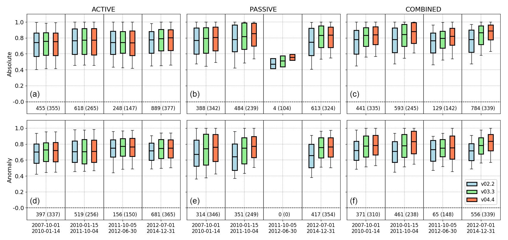
Figure 9Box plots of correlations against the unknown truth of measurements from the ACTIVE (a, d), PASSIVE (b, e) and COMBINED (c, f) products, both for absolute time series (a–c) and soil moisture anomalies (d–f). Box colours refer to the ESA CCI SM product versions v02.2, v03.3 and v04.4. The x axes represent different merging periods (see Fig. 2). Boxes represent the median and IQR, and whiskers represent the 10th and 90th percentiles of significant correlations (p<0.05) over all stations where at least 100 collocated measurements are available. The number of stations available for calculating the correlation statistics for a particular product and time period is shown below the zero line. The number in brackets shows the average number of collocated measurements available at each station for calculating correlation coefficients.
Table 4Median correlations against the unknown truth of absolute soil moisture time series and soil moisture anomalies from the ACTIVE, PASSIVE and COMBINED ESA CCI SM product versions v02.2, v03.3 and v04.4 in the latest four merging periods. Merging periods 1, 2, 3 and 4 refer to October 2007 to January 2010, January 2010 to October 2011, October 2011 to June 2012 and July 2012 to December 2014 (see Fig. 2).
Spatial statistics of the estimated correlations (Re) are shown in Fig. 9 and summarised in Table 4. Clear improvements for increasing ESA CCI SM product version are visible for the PASSIVE and the COMBINED products in almost all merging periods, both for absolute soil moisture time series and for anomalies. No significant anomaly correlations and significant absolute correlations from only four sites are available for the PASSIVE product in the merging period between October 2011 and June 2012, which is associated with the low data coverage of WindSat and SMOS that are used in this period, and the predominant frozen conditions during this time of the year, which lead to further masking of most data points. The lower quartile of anomaly correlations of the COMBINED product in the same merging period has slightly degraded from ESA CCI SM v3 to v4. This may be caused by an inaccurate VOD-based weight prediction in the v4 product as this merging period does not cover most of the summer and autumn retrievals, while weight prediction is based on annual-average VOD conditions. However, it may also just be a statistical artefact given the significantly reduced data coverage in this period and the reduced number of stations available to calculate correlation percentiles.
Only slight, non-significant changes are visible for the ACTIVE product, which is expected because only a single sensor is used and no statistical merging is applied that would be affected by changes between product versions. Also, the inclusion of MetOp-B observations as of ESA CCI SM v3 is unlikely to influence the results as only dates where all three ESA CCI SM product versions provide valid observations are considered in the analysis. Therefore, apparent changes originate mainly from differences in the L2 soil moisture retrieval algorithm version that has been used for ASCAT (see Table 1), more specifically from model parameter updates due to the time series extension.
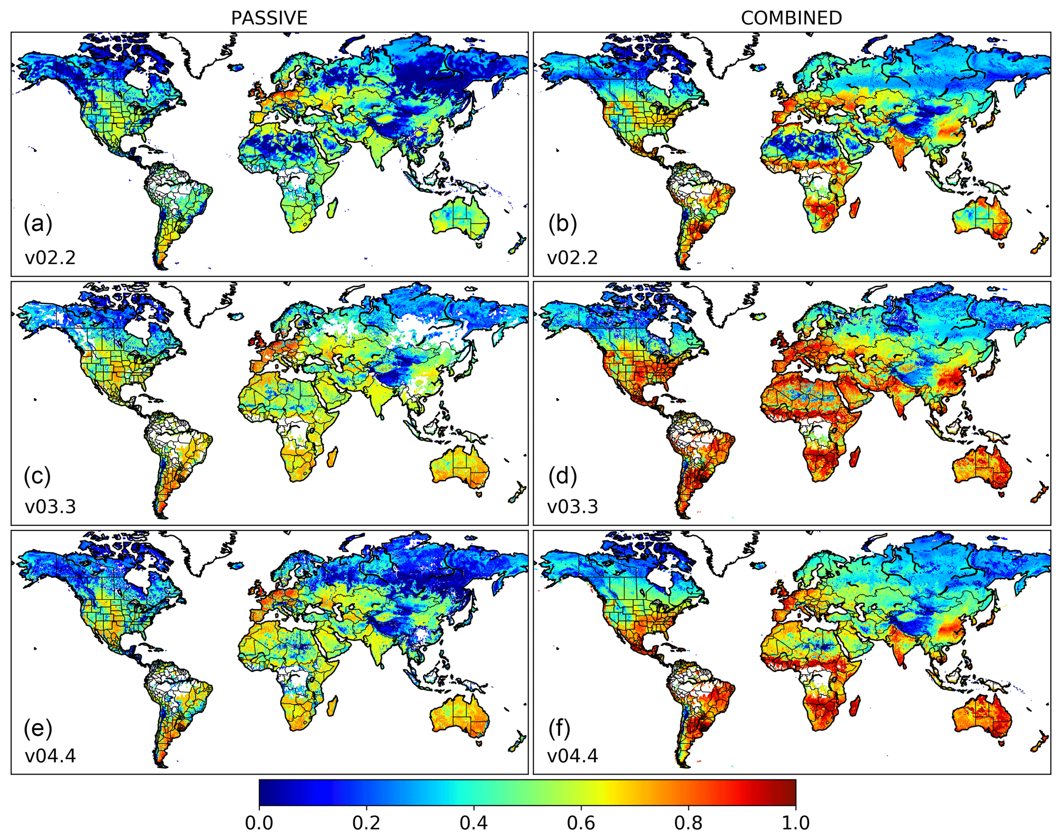
Figure 10Fraction of days during the latest four merging periods (October 2007 to December 2014), where the PASSIVE (a, c, e) and COMBINED (b, d, f) product versions v02.2 (a, b), v03.3 (c, d) and v04.4 (e, f) provide valid observations.
To complement the demonstration of ESA CCI SM product performance, Fig. 10 shows the fraction of days where the ESA CCI SM products provide valid soil moisture estimates. Only the PASSIVE and COMBINED products and only the latest four merging periods are considered because these are most affected by changes in the merging algorithm. Overall, there are many regions where the ESA CCI SM products provide valid observations almost every day. Areas with significantly reduced data coverage are mainly those with prolonged frozen periods, where soil moisture cannot be retrieved, and densely vegetated areas as well as regions with complex topography, where soil moisture retrieval is particularly challenging.
Data coverage significantly improved from ESA CCI SM v2 to v3 at most locations due to the introduction of the least squares merging scheme, which allowed more than one or two sensors to be merged on individual days. The quality control that was introduced into this merging scheme (based on p values and minimum-weight thresholds; see Sect. 6) has caused some spatial gaps in the PASSIVE product in v3 in already data-scarce regions where data quality of the passive sensors is generally poor (see Fig. 7). These gaps could be closed again by refining the masking scheme in v4 (see Sect. 7). Note, however, that this revised masking also has slightly reduced data coverage compared to v3 in some regions where bad observations have been sacrificed for the sake of overall data quality (see Fig. 9). Data coverage is expected to improve again in the upcoming product version 5.
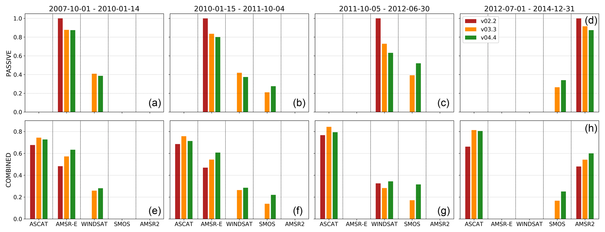
Figure 11Fractional contribution (y axis) of the individual sensors (x axis) to valid ESA CCI SM soil moisture estimates of the PASSIVE and COMBINED products (top to bottom) during the last four merging periods (left to right). Bar colours refer to the ESA CCI SM product versions v02.2, v03.3 and v04.4.
Figure 11 furthermore shows the average fraction of valid observations to which each individual sensor contributes during each day in each merging period, either alone or merged together (hence, the cumulative fractions of all sensors can be above unity). Note that Fig. 11 only provides information about the overall number of grid points to which each sensor contributes and not with which weight they contribute. Weights attributed to each sensor in product versions 2 and 3 are shown in Fig. 4. For version 4, this information cannot be summarised meaningfully as weights change dynamically each day depending on how many sensors provide valid observations at a particular location (see Sect. 7). However, since weights are derived from the uncertainties of the individual L2 soil moisture products, the SNRs shown in Fig. 7 are a direct (inverse) proxy for relative merging weights.
SMOS contributions are generally low due to excessive data masking in RFI-contaminated areas. By contrast, ASCAT soil moisture retrievals are not affected by RFI and they are also not masked under high-VOD conditions (as are all passive data sets; see Sect. 3). Therefore, ASCAT contributions are generally large. AMSR-E contributions decreased after v2 as both WindSat and SMOS observations became available to replace AMSR-E observations at some locations where they are deemed unreliable. Both WindSat and SMOS contributions further increased from v3 to v4 in most periods because of the refined relative weighting and data set masking.
Note that it is generally difficult to pinpoint the exact origin of all apparent patterns because they are caused by both changes in the L2 retrieval algorithms and their inherent quality control, as well as by changes in the different sensor masking procedures during the weight estimation within the least squares merging (i.e. the p-value-based mask and the applied minimum-weight threshold; see Sects. 6 and 7). For an exhaustive summary of comprehensive, dedicated validation studies for the various ESA CCI SM product versions, we refer the reader to Dorigo et al. (2015, 2017).
The soil moisture CDRs produced within the ESA CCI SM are freely available upon registration at http://www.esa-soilmoisture-cci.org/ or at the Centre for Environmental Data Analysis (CEDA) via http://dx.doi.org/10.5285/3729b3fbbb434930bf65d82f9b00111c (ESA CCI SM v2; Wagner et al., 2018), http://dx.doi.org/10.5285/b810601740bd4848b0d7965e6d83d26c (ESA CCI SM v3; Dorigo et al., 2018) and http://dx.doi.org/10.5285/dce27a397eaf47e797050c220972ca0e (ESA CCI SM v4; Dorigo et al., 2019). ISMN data are freely available upon registration at https://ismn.geo.tuwien.ac.at/ (last access: 17 May 2019).
The European Space Agency's Climate Change Initiative for Soil Moisture (ESA CCI SM) algorithm generates consistent, quality-controlled, long-term (1978–2018) soil moisture climate data records (CDRs) by harmonising and merging soil moisture retrievals from multiple satellites into (i) an active-microwave-based only (ACTIVE), (ii) a passive-microwave-based only (PASSIVE) and a (iii) combined active–passive (COMBINED) product. This paper reviews and discusses the science behind the three major ESA CCI SM merging algorithm versions:
-
ESA CCI SM v2 was used for all product releases between 2012 and 2016. This algorithm merges active and passive soil moisture retrievals by selecting either one of them alone or by computing the unweighted average of both based on their mutual correlation and average vegetation optical depth (VOD) conditions at a given location and time period.
-
ESA CCI SM v3 was released in early 2017, extended at the end of 2017 and used for the near-real-time Copernicus Climate Change Service (C3S) Soil Moisture CDR production up to version v201801. This algorithm uses a weighted-least-squares-based merging scheme, which is parameterised by triple collocation analysis (TCA)-based uncertainty estimates and uses correlation significance levels (p values) to fall back to a ternary decision scheme (active-only, passive-only, or an unweighted average) at grid cells and/or during time periods where TCA-based uncertainty estimates are deemed unreliable.
-
ESA CCI SM v4 was used to generate the product releases at the beginning and the end of 2018 and has been used for the C3S Soil Moisture CDR production since version v201812. This algorithm introduced a VOD-based polynomial regression to obtain global uncertainty estimates for all products (i.e. also in regions where TCA-based estimates are not reliable) and directly merges all active and passive L2 soil moisture retrievals into the COMBINED product (i.e. no longer the previously merged ACTIVE and PASSIVE products).
Harmonising soil moisture retrievals from active and passive microwave measurements from instruments which (i) operate at different wavelengths, polarisations and incidence angles; (ii) have diverging spatial, temporal and radiometric resolution; and (iii) are hardly ever well collocated in space and time is a heavily ill-posed problem. The ESA CCI SM merging algorithm is hence subject to continuous research and development. In the following, we summarise known issues that are currently under investigation and highlight improvements that are expected to be implemented in the next algorithm version (v5), which is foreseen to be released in 2019.
-
L2 data usage
-
Soil moisture retrievals from SMAP (Entekhabi et al., 2010) will be integrated into the next algorithm version v5. SMAP retrievals are expected to significantly enhance the ESA CCI SM performance from 2015 onwards due to its long wavelength (L-band) and remarkably high radiometric accuracy (Chen et al., 2018).
-
SSM/I and TMI data are not yet fully integrated. At midlatitudes, SSM/I data was disregarded in favour of TMI, and both products were cut off after the launch of the presumed better AMSR-E, because their low temporal coverage was assumed to render TCA-based uncertainty estimates (required for the least squares merging scheme) too unreliable (see Sect. 6.3). Nonetheless, their estimated uncertainties (see Fig. 7) suggest potentially useful complementary information even in the presence of the more recent missions.
-
In ESA CCI SM v2, WindSat is merely used for bridging the gap between the failure of AMSR-E and the launch of AMSR2. For this reason, WindSat data were only retrieved until mid-2012. However, due to L1 data availability issues, WindSat retrievals have not been extended since, even though uncertainty estimates for WindSat (see Fig. 7) suggest that more recent retrievals may benefit the ESA CCI SM product when integrated in the least squares merging scheme.
-
All ESA CCI SM products are sampled on a 0.25∘ regular grid and incorporate only L2 retrievals from sensors that operate at a comparable resolution. However, high-resolution soil moisture retrievals from synthetic aperture radar (SAR) instruments, in particular Envisat ASAR and Sentinel-1, are expected to provide useful complementary information either when upscaled to coarse resolution or for downscaling the ESA CCI SM products.
-
-
Data harmonisation
-
In current and previous product versions, AMSR-E and AMSR2 retrievals are treated as if they were perfectly intercalibrated, that is, no harmonisation between the two is applied. However, visual time series inspections as well as preliminary studies suggest that remaining biases are present, which should be removed before merging (Parinussa et al., 2015). The same may be the case for MetOp-A and MetOp-B ASCAT retrievals, even though no significant discrepancies have been found yet.
-
The CDF matching, which is used for harmonising L2 product climatologies, implicitly assumes that the considered data sets have an identical signal-to-noise ratio, which is hardly ever the case (see Fig. 7). Therefore, rescaling coefficients will most certainly be biased. TCA may provide an alternative approach for estimating optimal (in a least squares sense) scaling coefficients (Yilmaz and Crow, 2013).
-
For the sake of consistency, L2 soil moisture estimates in all ESA CCI SM product versions are retrieved using the WARP algorithm for active microwave measurements and the LPRM algorithm for passive microwave measurements (see Sect. 3). The selection of these two algorithms was based on an extensive round robin comparison between various retrieval models (Gruber et al., 2014; Mittelbach et al., 2014). However, these choices may be worth reassessing, especially due to the availability of new SMOS and SMAP products (O'Neill et al., 2018; Fernandez-Moran et al., 2017; Entekhabi et al., 2010).
-
-
Uncertainty estimation
-
In the current merging scheme (v4), uncertainties, and hence relative merging weights, are assumed to be (locally) stationary. That is, they are held constant during the entire time period for which TCA is applied. However, given their strong link with vegetation density, actual uncertainties are expected to vary significantly between seasons or with land cover change. Consequently, the estimation of non-stationary uncertainties could provide more accurate relative weightings on an intra-annual basis and thus a more efficient uncertainty reduction upon merging. Such time-variant uncertainty estimation, realised by decomposing the satellite time series into different frequency components and merging them separately (Draper and Reichle, 2015; Su and Ryu, 2015), is currently under investigation and foreseen to be integrated in a future release of the ESA CCI SM data set.
-
The statistical merging that was introduced in ESA CCI SM v3 is a weighted least squares implementation, which neglects possible error correlations across products. While such correlations are very likely to exist between the errors of the passive products they are usually not expected between errors of active and passive products, although the latter may be introduced by vegetation dynamics that are not completely removed in the retrieval (Gruber et al., 2016a; Zwieback et al., 2018) or imposed by the non-linear nature of the CDF matching (see below). However, unless the relative uncertainties of the merged products (with correlated errors) diverge by several orders of magnitude, non-zero error correlations will only cause suboptimal and not significantly incorrect relative weighting. Nonetheless, if existing error cross-correlations could be estimated and considered in a generalized least squares fashion (i.e. parameterising the currently neglected off-diagonal elements of the error covariance matrices), this could again lead to a significant performance improvement of the ESA CCI SM products. One option to do this could be through extended collocation analysis (ECA; Gruber et al., 2016a), which is currently the only potentially available method for estimating error correlations between large-scale soil moisture products. However, the method has not yet been validated on a global scale and has been found to be particularly susceptible to small sample sizes, although this issue is expected to be mitigated by the progressively increasing data coverage of currently available missions.
-
The polynomial regression for predicting uncertainties from VOD, which was introduced in ESA CCI SM v4, is based on long-term average C-band VOD estimates retrieved from AMSR-E. However, the functional relationship between uncertainties and VOD may be different for the Ku-band retrievals from SSM/I, for the X-band retrievals from TMI and AMSR-E and for the L-band retrievals from SMOS and SMAP, especially when considering their intra-annual variability. Therefore, VOD-based uncertainty predictions for individual sensors may be more accurate when obtained from a regression with VOD estimates in their respective frequency band and/or in a temporally dynamic manner.
-
The p-value mask for excluding individual data sets that was introduced in ESA CCI SM v4 was implemented on a relatively conservative ad hoc basis and a more thorough evaluation and refinement is pending. For example, absolute or relative signal-to-noise ratios and/or relative weight differences may help to better balance temporal measurement density and data quality.
-
-
Model dependency
-
So far, climatologies are harmonised (for the COMBINED product) by CDF matching individual products against the GLDAS Noah land surface model. This may impact long-term trend analyses because, even though CDF matching generally preserves the direction of an existing trend in a rescaled product, it can change its magnitude (Liu et al., 2012). That is, the rescaling against GLDAS Noah can cause trends found in the harmonised ESA CCI SM product to appear stronger or weaker than they actually are. Moreover, the non-linear nature of the CDF matching may introduce spurious error correlations, which could be problematic for TCA (see above) but also when evaluating the ESA CCI SM data set against other land surface models such as ERA-Interim/Land or MERRA2, which hampers a comprehensive large-scale validation of the product. A potential alternative could be the use of TCA-based linear rescaling, which was found to be potentially superior to CDF matching, especially for data merging if SNRs of different products are not equal (Yilmaz and Crow, 2013).
-
Apart from serving as a scaling reference, GLDAS Noah is also used as a third data set to complement the data triplet used for TCA. This, per se, would not introduce spurious correlations between the merged ESA CCI SM product and the model because – in theory – each data set merely serves as an independent “instrument” to isolate the individual error variabilities from the total variabilities present in each product (Su et al., 2014). However, this isolation is realised by using the jointly observed variability from the three products as a reference for the true soil moisture variability (hence the requirement of uncorrelated errors) to derive the individual error variances as deviations from this jointly observed true soil moisture signal. Consequently, mismatches in the spatial representation (i.e. horizontal and vertical resolution) and temporal collocation may cause real soil moisture signals that are not captured by all three data sets (such as precipitation events not present in the model forcing) or signals that are seen by the satellite data sets but not represented in the land surface model (such as irrigation; Brocca et al., 2018) to be interpreted as representativeness errors or – looking from a different angle – as spurious error correlations (Miralles et al., 2010; Vogelzang and Stoffelen, 2012; Gruber et al., 2013, 2016b). This could again lead to biases in the estimated uncertainties and hence merging weights. It is therefore desirable to avoid the use of a land surface model altogether, not only in the harmonisation process but also in TCA, e.g. by replacing it with a lagged version of the satellite products (Su et al., 2014).
-
The authors declare that they have no conflict of interest.
The methods reported on within this paper are further integrated within the production system providing TCDR/ICDR to the Copernicus Climate Change Service (C3S) implemented by ECMWF on behalf of the European Commission. We thank the ISMN data providers for sharing their data with the community. Analyses in this paper are based on data from the following networks: AMMA-CATCH (http://www.amma-catch.org/; Pellarin et al., 2009), ARM (http://www.arm.gov/), AWDN (http://www.hprcc.unl.edu/awdn.php), BNZ-LTER (http://www.lter.uaf.edu/), CARBOAFRICA (Ardö, 2012), COSMOS (http://coSMOS.hwr.arizona.edu/; Zreda et al., 2012), CTP_SMTMN (http://dam.itpcas.ac.cn/rs/?q=data\#CTP-SMTMN; Yang et al., 2013) , DAHRA (Tagesson et al., 2015), FLUXNET-AMERIFLUX (http://ameriflux.lbl.gov/), FMI (http://fmiarc.fmi.fi/), FR_Aqui, GTK, HOBE (http://www.hobe.dk/; Bircher et al., 2012), ICN (http://www.isws.illinois.edu/warm/; Hollinger and Isard, 1994), IIT_KANPUR (http://www.iitk.ac.in/), MAQU (Su et al., 2011), MOL-RAO (http://www.dwd.de/mol), ORACLE (http://gisoracle.irstea.fr/?lang=en;https://bdoh.irstea.fr/ORACLE/), OZNET (http://www.oznet.org.au/; Smith et al., 2012), PBO_H2O (Larson et al., 2008), REMEDHUS (http://campus.usal.es/~hidrus/, RISMA (http://aafc.fieldvision.ca/; Ojo et al., 2015), RSMN (http://assimo.meteoromania.ro/, SCAN (http://www.wcc.nrcs.usda.gov/), SMOSMANIA (http://www.hymex.org/; Albergel et al., 2008), SNOTEL (http://www.wcc.nrcs.usda.gov/; Leavesley et al., 2008), SOILSCAPE (http://soilscape.usc.edu/; Moghaddam et al., 2010), SWEX_POLAND (Marczewski et al., 2010), TERENO (http://teodoor.icg.kfa-juelich.de/; Zacharias et al., 2011), UDC_SMOS (http://www.geographie.uni-muenchen.de/department/fiona/forschung/projekte/index.php?projekt_id=103; Schlenz et al., 2012), UMBRIA (http://www.cfumbria.it/; Brocca et al., 2011), UMSUOL (http://www.arpa.emr.it/sim/), USCRN (http://www.ncdc.noaa.gov/crn/; Bell et al., 2013), USDA-ARS (https://www.ars.usda.gov/; Jackson et al., 2010) and WSMN. Date of last access for all links is 17 May 2019.
This research has been supported by the eartH2Observe project of the European Union's Seventh Framework Programme (grant no. 603608), the ESA's Climate Change Initiative (CCI) for soil moisture (grant no. 4000104814/11/I-NB), and the KU Leuven C1 internal fund (grant no. C14/16/045).
This paper was edited by David Carlson and reviewed by Amen Al-Yaari and two anonymous referees.
Aitkin, A.: On least squares and linear combination of observations, P. Roy. Soc. Edinb., 55, 42–48, 1935. a
Albergel, C., Rüdiger, C., Pellarin, T., Calvet, J.-C., Fritz, N., Froissard, F., Suquia, D., Petitpa, A., Piguet, B., and Martin, E.: From near-surface to root-zone soil moisture using an exponential filter: an assessment of the method based on in-situ observations and model simulations, Hydrol. Earth Syst. Sci., 12, 1323–1337, https://doi.org/10.5194/hess-12-1323-2008, 2008. a
Al-Yaari, A., Wigneron, J.-P., Ducharne, A., Kerr, Y., Wagner, W., De Lannoy, G., Reichle, R., Al Bitar, A., Dorigo, W., Richaume, P., and Mialon, A.: Global-scale comparison of passive (SMOS) and active (ASCAT) satellite based microwave soil moisture retrievals with soil moisture simulations (MERRA-Land), Remote Sens. Environ., 152, 614–626, https://doi.org/10.1016/j.rse.2014.07.013, 2014. a
Ardö, J.: A 10-year dataset of basic meteorology and soil properties in Central Sudan, Dataset Papers in Science, 2013, 297973, https://doi.org/10.7167/2013/297973, 2012. a
Bell, J. E., Palecki, M. A., Baker, C. B., Collins, W. G., Lawrimore, J. H., Leeper, R. D., Hall, M. E., Kochendorfer, J., Meyers, T. P., Wilson, T., and Diamond, H. J.: US Climate Reference Network soil moisture and temperature observations, J. Hydrometeorol., 14, 977–988, https://doi.org/10.1175/JHM-D-12-0146.1, 2013. a
Bircher, S., Skou, N., Jensen, K. H., Walker, J. P., and Rasmussen, L.: A soil moisture and temperature network for SMOS validation in Western Denmark, Hydrol. Earth Syst. Sci., 16, 1445–1463, https://doi.org/10.5194/hess-16-1445-2012, 2012. a
Brocca, L., Hasenauer, S., Lacava, T., Melone, F., Moramarco, T., Wagner, W., Dorigo, W., Matgen, P., Martinez-Fernandez, J., Llorens, P., Latron, J., Martin, C., and Bittelli, M.: Soil moisture estimation through ASCAT and AMSR-E sensors: An intercomparison and validation study across Europe, Remote Sens. Environ., 115, 3390–3408, 2011. a
Brocca, L., Tarpanelli, A., Filippucci, P., Dorigo, W., Zaussinger, F., Gruber, A., and Fernández-Prieto, D.: How much water is used for irrigation? A new approach exploiting coarse resolution satellite soil moisture products, Int. J. Appl. Earth Obs., 73, 752–766, https://doi.org/10.1016/j.jag.2018.08.023, 2018. a
Chen, F., Crow, W. T., Colliander, A., Cosh, M. H., Jackson, T. J., Bindlish, R., Reichle, R. H., Chan, S. K., Bosch, D. D., Starks, P. J., Goodrich, D. C., and Seyfried, M. S.: Application of triple collocation in ground-based validation of Soil Moisture Active/Passive (SMAP) level 2 data products, IEEE J. Sel. Top. Appl., 10, 489–502, https://doi.org/10.1109/JSTARS.2016.2569998, 2017. a, b
Chen, F., Crow, W. T., Bindlish, R., Colliander, A., Burgin, M. S., Asanuma, J., and Aida, K.: Global-scale evaluation of SMAP, SMOS and ASCAT soil moisture products using triple collocation, Remote Sens. Environ., 214, 1–13, 2018. a
Chung, D., Dorigo, W., Hahn, S., Melzer, T., Paulik, C., Reimer, C., Vreugdenhil, M., Wagner, W., Kidd, R., Gruber, A., and Scanlon, T.: Algorithm Theoretical Baseline Document (ATBD) D2.1 Version 04.4, Merging Active and Passive Soil Moisture Retrievals, ESA CCI Soil Moisture, available at: http://dap.ceda.ac.uk/thredds/fileServer/neodc/esacci/soil_moisture/docs/v04.4/CCI2_Soil_Moisture_DL2.1_ATBD_v4.4_04_merging.pdf (last access: 17 May 2019), 2018a. a
Chung, D., Dorigo, W., Reimer, C., Hahn, S., Melzer, T., Paulik, C., Vreugdenhil, M., Wagner, W., and Kidd, R.: Algorithm Theoretical Baseline Document (ATBD) D2.1 Version 04.4, Active Soil Moisture Retrievals, ESA CCI Soil Moisture, available at: http://dap.ceda.ac.uk/thredds/fileServer/neodc/esacci/soil_moisture/docs/v04.4/CCI2_Soil_Moisture_DL2.1_ATBD_v4.4_02_active.pdf (last access: 17 May 2019), 2018b. a
de Jeu, R. A. M., Dorigo, W., van der Schalie, R., Chung, D., Wagner, W., and Kidd, R.: Algorithm Theoretical Baseline Document (ATBD) D2.1 Version 04.4, Soil Moisture Retrievals from Passive Microwave Sensors, ESA CCI Soil Moisture, available at: http://dap.ceda.ac.uk/thredds/fileServer/neodc/esacci/soil_moisture/docs/v04.4/CCI2_Soil_Moisture_DL2.1_ATBD_v4.4_03_passive.pdf (last access: 17 May 2019), 2018. a
de Nijs, A. H., Parinussa, R. M., de Jeu, R. A., Schellekens, J., and Holmes, T. R.: A Methodology to Determine Radio-Frequency Interference in AMSR2 Observations, IEEE T. Geosci. Remote, 53, 5148–5159, 2015. a
Dorigo, W. A., Scipal, K., Parinussa, R. M., Liu, Y. Y., Wagner, W., de Jeu, R. A. M., and Naeimi, V.: Error characterisation of global active and passive microwave soil moisture datasets, Hydrol. Earth Syst. Sci., 14, 2605–2616, https://doi.org/10.5194/hess-14-2605-2010, 2010. a, b
Dorigo, W., van Oevelen, P., Wagner, W., Drusch, M., Mecklenburg, S., Robock, A., and Jackson, T.: A New International Network for in Situ Soil Moisture Data, Eos Transactions AGU, 92, 141–142, 2011a. a
Dorigo, W. A., Wagner, W., Hohensinn, R., Hahn, S., Paulik, C., Xaver, A., Gruber, A., Drusch, M., Mecklenburg, S., van Oevelen, P., Robock, A., and Jackson, T.: The International Soil Moisture Network: a data hosting facility for global in situ soil moisture measurements, Hydrol. Earth Syst. Sci., 15, 1675–1698, https://doi.org/10.5194/hess-15-1675-2011, 2011b. a
Dorigo, W., Xaver, A., Vreugdenhil, M., Gruber, A., A, H., Sanchis-Dufau, A., Zamojski, D., Cordes, C., Wagner, W., and Drusch, M.: Global Automated Quality Control of In Situ Soil Moisture Data from the International Soil Moisture Network, Vadose Zone J., 12, https://doi.org/10.2136/vzj2012.0097, 2013. a
Dorigo, W., Gruber, A., De Jeu, R., Wagner, W., Stacke, T., Loew, A., Albergel, C., Brocca, L., Chung, D., Parinussa, R., and Kidd, R.: Evaluation of the ESA CCI soil moisture product using ground-based observations, Remote Sens. Environ., 162, 380–395, 2015. a, b, c
Dorigo, W., Wagner, W., Albergel, C., Albrecht, F., Balsamo, G., Brocca, L., Chung, D., Ertl, M., Forkel, M., Gruber, A., Haas, E., Hamer, P., Hirschi, M., Ikonen, J., de Jeu, R., Kidd, R., Lahoz, W., Liu, Y., Miralles, D., Mistelbauer, T., Nicolai-Shaw, N., Parinussa, R., Reimer, C., van der Schalie, R., Seneviratne, S., Smolander, T., and Lecomte, P.: ESA CCI Soil Moisture for improved Earth system understanding: state-of-the art and future directions, Remote Sens. Environ., 203, 185–215, https://doi.org/10.1016/j.rse.2017.07.001, 2017. a, b, c, d
Dorigo, W., Wagner, W., Gruber, A., Scanlon, T., Hahn, S., Kidd, R., Paulik, C., Reimer, C., Van der Schalie, R., and De Jeu, R.: ESA Soil Moisture Climate Change Initiative (Soil_Moisture_cci): Version 03.3 data collection, Centre for Environmental Data Analysis, https://doi.org/10.5285/b810601740bd4848b0d7965e6d83d26c, 2018. a, b, c, d
Dorigo, W., Wagner, W., Gruber, A., Scanlon, T., Hahn, S., Kidd, R., Paulik, C., Reimer, C., Van der Schalie, R., Preimesberger, W., and De Jeu, R.: ESA Soil Moisture Climate Change Initiative (Soil_Moisture_cci): Version 04.4 data collection, Centre for Environmental Data Analysis, https://doi.org/10.5285/dce27a397eaf47e797050c220972ca0e, 2019. a, b, c, d
Draper, C. and Reichle, R.: The impact of near-surface soil moisture assimilation at subseasonal, seasonal, and inter-annual timescales, Hydrol. Earth Syst. Sci., 19, 4831–4844, https://doi.org/10.5194/hess-19-4831-2015, 2015. a
Efron, B.: Bayes' theorem in the 21st century, Science, 340, 1177–1178, 2013. a
Entekhabi, D., Njoku, E., O'Neill, P., Kellogg, K., Crow, W., Edelstein, W., Entin, J., Goodman, S., Jackson, T., Johnson, J., Kimball, J., Piepmeier, J., Koster, R., Martin, N., McDonald, K., Moghaddam, M., Moran, S., Reichle, R., Shi, J., Spencer, M., Thurman, S., Tsang, L., and Van Zyl, J.: The Soil Moisture Active Passive (SMAP) Mission, P. IEEE, 98, 704–716, https://doi.org/10.1109/JPROC.2010.2043918, 2010. a, b
Fernandez-Moran, R., Al-Yaari, A., Mialon, A., Mahmoodi, A., Al Bitar, A., De Lannoy, G., Rodriguez-Fernandez, N., Lopez-Baeza, E., Kerr, Y., and Wigneron, J.-P.: SMOS-IC: An alternative SMOS soil moisture and vegetation optical depth product, Remote Sensing, 9, 457, https://doi.org/10.3390/rs9050457, 2017. a
Gelb, A.: Applied optimal estimation, MIT press, Cambridge, Mass, USA, 1974. a
Gruber, A., Dorigo, W., Zwieback, S., Xaver, A., and Wagner, W.: Characterizing Coarse-Scale Representativeness of in situ Soil Moisture Measurements from the International Soil Moisture Network, Vadose Zone J., 12, https://doi.org/10.2136/vzj2012.0170, 2013. a, b
Gruber, A., Paloscia, S., Santi, E., Notarnicola, C., Pasolli, L., Smolander, T., Pulliainen, J., Mittelbach, H., Dorigo, W., and Wagner, W.: Round Robin evaluation of soil moisture retrieval models for the MetOp-A ASCAT instrument, in: EGU General Assembly Conference Abstracts, 27 April–2 May 2014, Vienna, Austria, vol. 16, 2014. a
Gruber, A., Su, C.-H., Crow, W., Zwieback, S., Dorigo, W., and Wagner, W.: Estimating error cross-correlations in soil moisture data sets using extended collocation analysis, J. Geophys. Res.-Atmos., 121, 1208–1219, https://doi.org/10.1002/2015JD024027, 2016a. a, b, c
Gruber, A., Su, C.-H., Zwieback, S., Crow, W., Dorigo, W., and Wagner, W.: Recent advances in (soil moisture) triple collocation analysis, Int. J. Appl. Earth Obs., 45, 200–211, https://doi.org/10.1016/j.jag.2015.09.002, 2016b. a, b, c, d, e, f, g, h, i
Gruber, A., Dorigo, W. A., Crow, W., and Wagner, W.: Triple Collocation-Based Merging of Satellite Soil Moisture Retrievals, IEEE T. Geosci. Remote, 55, 6780–6792, 2017. a, b, c, d, e, f, g
Gruber, A., Crow, W., and Dorigo, W.: Assimilation of spatially sparse in situ soil moisture networks into a continuous model domain, Water Resour. Res., 54, 1353–1367, https://doi.org/10.1002/2017WR021277, 2018. a
Hollinger, S. E. and Isard, S. A.: A soil moisture climatology of Illinois, J. Climate, 7, 822–833, 1994. a
Holmes, T., De Jeu, R., Owe, M., and Dolman, A.: Land surface temperature from Ka band (37 GHz) passive microwave observations, J. Geophys. Res.-Atmos., 114, D04113, https://doi.org/10.1029/2008JD010257, 2009. a
Jackson, T., Cosh, M., Bindlish, R., Starks, P., Bosch, D., Seyfried, M., Goodrich, D., Moran, M., and Du, J.: Validation of Advanced Microwave Scanning Radiometer Soil Moisture Products, IEEE T. Geosci. Remote, 48, 4256–4272, 2010. a
Larson, K. M., Small, E. E., Gutmann, E. D., Bilich, A. L., Braun, J. J., and Zavorotny, V. U.: Use of GPS receivers as a soil moisture network for water cycle studies, Geophys. Res. Lett., 35, L24405, https://doi.org/10.1029/2008GL036013, 2008. a
Leavesley, G., David, O., Garen, D., Lea, J., Marron, J., Pagano, T., Perkins, T., and Strobel, M.: A modeling framework for improved agricultural water supply forecasting, in: AGU Fall Meeting Abstracts, 15–19 December 2008, San Francisco, USA, vol. 1, 0497, 2008. a
Li, L., Njoku, E. G., Im, E., Chang, P. S., and Germain, K. S.: A preliminary survey of radio-frequency interference over the US in Aqua AMSR-E data, IEEE T. Geosci. Remote, 42, 380–390, 2004. a
Liu, Y., Dorigo, W., Parinussa, R., de Jeu, R., Wagner, W., McCabe, M., Evans, J., and van Dijk, A.: Trend-preserving blending of passive and active microwave soil moisture retrievals, Remote Sens. Environ., 123, 280–297, https://doi.org/10.1016/j.rse.2012.03.014, 2012. a, b, c, d, e, f, g, h, i, j, k, l, m, n
Liu, Y. Y., Parinussa, R. M., Dorigo, W. A., De Jeu, R. A. M., Wagner, W., van Dijk, A. I. J. M., McCabe, M. F., and Evans, J. P.: Developing an improved soil moisture dataset by blending passive and active microwave satellite-based retrievals, Hydrol. Earth Syst. Sci., 15, 425–436, https://doi.org/10.5194/hess-15-425-2011, 2011. a, b, c, d, e, f, g, h, i, j
Marczewski, W., Slominski, J., Slominska, E., Usowicz, B., Usowicz, J., Romanov, S., Maryskevych, O., Nastula, J., and Zawadzki, J.: Strategies for validating and directions for employing SMOS data, in the Cal-Val project SWEX (3275) for wetlands, Hydrol. Earth Syst. Sci. Discuss., 7, 7007–7057, https://doi.org/10.5194/hessd-7-7007-2010, 2010. a
McColl, K. A., Vogelzang, J., Konings, A. G., Entekhabi, D., Piles, M., and Stoffelen, A.: Extended triple collocation: Estimating errors and correlation coefficients with respect to an unknown target, Geophys. Res. Lett., 41, 6229–6236, https://doi.org/10.1002/2014GL061322, 2014. a, b
Meesters, A. G., De Jeu, R. A., and Owe, M.: Analytical derivation of the vegetation optical depth from the microwave polarization difference index, IEEE Geosci. Remote S., 2, 121–123, 2005. a
Miralles, D. G., Crow, W. T., and Cosh, M. H.: Estimating Spatial Sampling Errors in Coarse-Scale Soil Moisture Estimates Derived from Point-Scale Observations, J. Hydrometeorol., 11, 1423–1429, https://doi.org/10.1175/2010JHM1285.1, 2010. a, b
Mittelbach, H., Hirschi, M., Nicolai-Shaw, N., Gruber, A., Dorigo, W., de Jeu, R., Parinussa, R., Jones, L. A., Wagner, W., and Seneviratne, S. I.: A Round Robin evaluation of AMSR-E soil moisture retrievals, in: EGU General Assembly Conference Abstracts, 27 April–2 May 2014, Vienna, Austria, vol. 16, 2014. a
Mo, T., Choudhury, B., Schmugge, T., Wang, J., and Jackson, T.: A model for microwave emission from vegetation-covered fields, J. Geophys. Res.-Oceans, 87, 11229–11237, 1982. a
Moghaddam, M., Entekhabi, D., Goykhman, Y., Li, K., Liu, M., Mahajan, A., Nayyar, A., Shuman, D., and Teneketzis, D.: A wireless soil moisture smart sensor web using physics-based optimal control: Concept and initial demonstrations, IEEE J. Sel. Top. Appl., 3, 522–535, 2010. a
Nachtergaele, F. and Batjes, N.: Harmonized world soil database, FAO, available at: http://www.fao.org/soils-portal/soil-survey/soil-maps-and-databases/harmonized-world-soil-database-v12/en/ (last access: 17 May 2019), 2012. a
Naeimi, V., Scipal, K., Bartalis, Z., Hasenauer, S., and Wagner, W.: An improved soil moisture retrieval algorithm for ERS and METOP scatterometer observations, IEEE T. Geosci. Remote, 47, 1999–2013, https://doi.org/10.1109/TGRS.2008.2011617, 2009. a, b
Naeimi, V., Paulik, C., Bartsch, A., Wagner, W., Kidd, R., Park, S.-E., Elger, K., and Boike, J.: ASCAT Surface State Flag (SSF): Extracting information on surface freeze/thaw conditions from backscatter data using an empirical threshold-analysis algorithm, IEEE T. Geosci. Remote, 50, 2566–2582, https://doi.org/10.1109/TGRS.2011.2177667, 2012. a
Ojo, E. R., Bullock, P. R., L'Heureux, J., Powers, J., McNairn, H., and Pacheco, A.: Calibration and evaluation of a frequency domain reflectometry sensor for real-time soil moisture monitoring, Vadose Zone J., 14, https://doi.org/10.2136/vzj2014.08.0114, 2015. a
O'Neill, P., Chan, S., Njoku, E., Jackson, T., and Blindish, R.: SMAP L2 Radiometer Half-Orbit 36 km EASE-Grid Soil Moisture, Version 5, Boulder, Colorado USA. NASA National Snow and ice Data Center Distributed Active Archive Center, https://doi.org/10.5067/SODMLCE6LGLL, 2018. a
Owe, M., de Jeu, R., and Holmes, T.: Multisensor historical climatology of satellite-derived global land surface moisture, J. Geophys. Res.-Earth, 113, F01002, https://doi.org/10.1029/2007JF000769, 2008. a
Parinussa, R. M., Meesters, A. G., Liu, Y. Y., Dorigo, W., Wagner, W., and De Jeu, R. A.: Error estimates for near-real-time satellite soil moisture as derived from the land parameter retrieval model, IEEE Geosci. Remote S., 8, 779–783, 2011. a
Parinussa, R. M., Holmes, T. R., and de Jeu, R. A.: Soil moisture retrievals from the WindSat spaceborne polarimetric microwave radiometer, IEEE T. Geosci. Remote, 50, 2683–2694, 2012. a
Parinussa, R. M., Holmes, T. R., Wanders, N., Dorigo, W. A., and de Jeu, R. A.: A preliminary study toward consistent soil moisture from AMSR2, J. Hydrometeorol., 16, 932–947, 2015. a, b
Pellarin, T., Laurent, J.-P., Cappelaere, B., Decharme, B., Descroix, L., and Ramier, D.: Hydrological modelling and associated microwave emission of a semi-arid region in South-western Niger, J. Hydrol., 375, 262–272, 2009. a
Rodell, M., Houser, P., Jambor, U. E. A., Gottschalck, J., Mitchell, K., Meng, C., Arsenault, K., Cosgrove, B., Radakovich, J., Bosilovich, M., Entin, J., Walker, J., Lohmann, D., and Toll, D.: The global land data assimilation system, B. Am. Meteorol. Soc., 85, 381–394, https://doi.org/10.1175/BAMS-85-3-381, 2004. a
Schlenz, F., Dall'Amico, J. T., Loew, A., and Mauser, W.: Uncertainty assessment of the SMOS validation in the upper Danube catchment, IEEE T. Geosci. Remote,, 50, 1517–1529, 2012. a
Scipal, K., Holmes, T., de Jeu, R., Naeimi, V., and Wagner, W.: A possible solution for the problem of estimating the error structure of global soil moisture data sets, Geophys. Res. Lett., 35, L24403, https://doi.org/10.1029/2008GL035599, 2008. a
Smith, A., Walker, J., Western, A., Young, R., Ellett, K., Pipunic, R., Grayson, R., Siriwardena, L., Chiew, F., and Richter, H.: The Murrumbidgee soil moisture monitoring network data set, Water Resour. Res., 48, W07701, https://doi.org/10.1029/2012WR011976, 2012. a
Stoffelen, A.: Toward the true near-surface wind speed: Error modeling and calibration using triple collocation, J. Geophys. Res., 103, 7755–7766, https://doi.org/10.1029/97JC03180, 1998. a
Su, C.-H. and Ryu, D.: Multi-scale analysis of bias correction of soil moisture, Hydrol. Earth Syst. Sci., 19, 17–31, https://doi.org/10.5194/hess-19-17-2015, 2015. a
Su, C.-H., Ryu, D., Crow, W. T., and Western, A. W.: Beyond triple collocation: Applications to soil moisture monitoring, J. Geophys. Res.-Atmos., 119, 6419–6439, 2014. a, b, c
Su, Z., Wen, J., Dente, L., van der Velde, R., Wang, L., Ma, Y., Yang, K., and Hu, Z.: The Tibetan Plateau observatory of plateau scale soil moisture and soil temperature (Tibet-Obs) for quantifying uncertainties in coarse resolution satellite and model products, Hydrol. Earth Syst. Sci., 15, 2303–2316, https://doi.org/10.5194/hess-15-2303-2011, 2011. a
Tagesson, T., Fensholt, R., Guiro, I., Rasmussen, M. O., Huber, S., Mbow, C., Garcia, M., Horion, S., Sandholt, I., Holm-Rasmussen, B., Göttsche, F., Ridler, M.-E., Olén, N., Olsen, J., Ehammer, A., Madsen, M., Olesen, F., and Ardö, J: Ecosystem properties of semiarid savanna grassland in West Africa and its relationship with environmental variability, Glob. Change Biol., 21, 250–264, 2015. a
Ulaby, F. T., Long, D. G., Blackwell, W. J., Elachi, C., Fung, A. K., Ruf, C., Sarabandi, K., Zebker, H. A., and Van Zyl, J.: Microwave radar and radiometric remote sensing, vol. 4, University of Michigan Press, Ann Arbor, USA, 2014. a
van der Schalie, R., Kerr, Y. H., Wigneron, J.-P., Rodríguez-Fernández, N. J., Al-Yaari, A., and de Jeu, R. A.: Global SMOS soil moisture retrievals from the land parameter retrieval model, Int. J. Appl. Earth Obs., 45, 125–134, 2016. a
van der Schalie, R., De Jeu, R. A., Kerr, Y., Wigneron, J.-P., Rodríguez-Fernández, N. J., Al-Yaari, A., Parinussa, R. M., Mecklenburg, S., and Drusch, M.: The merging of radiative transfer based surface soil moisture data from SMOS and AMSR-E, Remote Sens. Environ., 189, 180–193, 2017. a
van der Schalie, R., de Jeu, R., Parinussa, R., Rodríguez-Fernández, N., Kerr, Y., Al-Yaari, A., Wigneron, J.-P., and Drusch, M.: The Effect of Three Different Data Fusion Approaches on the Quality of Soil Moisture Retrievals from Multiple Passive Microwave Sensors, Remote Sensing, 10, 107, https://doi.org/10.3390/rs10010107, 2018. a
Vogelzang, J. and Stoffelen, A.: Triple collocation, EUMETSAT Report, available at: https://www.researchgate.net/publication/314263507_Triple_collocation (last access: 17 May 2019), 2012. a
Vreugdenhil, M., Dorigo, W. A., Wagner, W., de Jeu, R. A., Hahn, S., and van Marle, M. J.: Analyzing the Vegetation Parameterization in the TU-Wien ASCAT Soil Moisture Retrieval, IEEE T. Geosci. Remote, 54, 3513–3531, 2016. a
Wagner, W., Lemoine, G., and Rott, H.: A Method for Estimating Soil Moisture from ERS Scatterometer and Soil Data, Remote Sens. Environ., 70, 191–207, https://doi.org/10.1016/S0034-4257(99)00036-X, 1999. a
Wagner, W., Dorigo, W., de Jeu, R., Fernandez, D., Benveniste, J., Haas, E., and Ertl, M.: Fusion of active and passive microwave observations to create an essential climate variable data record on soil moisture, ISPRS Annals of the Photogrammetry, Remote Sensing and Spatial Information Sciences (ISPRS Annals), 7, 315–321, 2012. a
Wagner, W., Dorigo, W., Chung, D., Gruber, A., Hahn, S., Kidd, R., Liu, Y., Mistelbauer, T., Parinussa, R., Paulik, C., Reimer, C., Van der Schalie, R., De Jeu, R., Melzer, T., and Vreugdenhil, M.: ESA Soil Moisture Climate Change Initiative (Soil_Moisture_cci): Version 02.2 data collection, Centre for Environmental Data Analysis, https://doi.org/10.5285/3729b3fbbb434930bf65d82f9b00111c, 2018. a, b, c, d
Yang, K., Qin, J., Zhao, L., Chen, Y., Tang, W., Han, M., Chen, Z., Lv, N., Ding, B., Wu, H., and Lin, C.: A multiscale soil moisture and freeze–thaw monitoring network on the third pole, B. Am. Meteorol. Soc., 94, 1907–1916, 2013. a
Yilmaz, M. T. and Crow, W. T.: The Optimality of Potential Rescaling Approaches in Land Data Assimilation., J. Hydrometeorol., 14, 650–660, https://doi.org/10.1175/JHM-D-12-052.1, 2013. a, b
Zacharias, S., Bogena, H., Samaniego, L., Mauder, M., Fuß, R., Pütz, T., Frenzel, M., Schwank, M., Baessler, C., Butterbach-Bahl, K., Bens, O., Borg, E., Brauer, A., Dietrich, P., Hajnsek, I., Helle, G., Kiese, R., Kunstmann, H., Klotz, S., Munch, J., Papen, H., Priesack, E., Schmid, H., Steinbrecher, R., Rosenbaum, U., Teutsch, G., and Vereecken, H.: A network of terrestrial environmental observatories in Germany, Vadose Zone J., 10, 955–973, 2011. a
Zreda, M., Shuttleworth, W. J., Zeng, X., Zweck, C., Desilets, D., Franz, T., and Rosolem, R.: COSMOS: the COsmic-ray Soil Moisture Observing System, Hydrol. Earth Syst. Sci., 16, 4079–4099, https://doi.org/10.5194/hess-16-4079-2012, 2012. a
Zwieback, S., Scipal, K., Dorigo, W., and Wagner, W.: Structural and statistical properties of the collocation technique for error characterization, Nonlin. Processes Geophys., 19, 69–80, https://doi.org/10.5194/npg-19-69-2012, 2012. a
Zwieback, S., Colliander, A., Cosh, M. H., Martínez-Fernández, J., McNairn, H., Starks, P. J., Thibeault, M., and Berg, A.: Estimating time-dependent vegetation biases in the SMAP soil moisture product, Hydrol. Earth Syst. Sci., 22, 4473–4489, https://doi.org/10.5194/hess-22-4473-2018, 2018. a, b
- Abstract
- Introduction
- Evolution of the ESA CCI SM merging algorithm
- Input data and preprocessing
- ESA CCI SM v2
- On the statistical optimality of data merging
- ESA CCI SM v3
- ESA CCI SM v4
- Product evaluation
- Data availability
- Conclusions
- Competing interests
- Acknowledgements
- Financial support
- Review statement
- References
The requested paper has a corresponding corrigendum published. Please read the corrigendum first before downloading the article.
- Article
(5016 KB) - Full-text XML
- Abstract
- Introduction
- Evolution of the ESA CCI SM merging algorithm
- Input data and preprocessing
- ESA CCI SM v2
- On the statistical optimality of data merging
- ESA CCI SM v3
- ESA CCI SM v4
- Product evaluation
- Data availability
- Conclusions
- Competing interests
- Acknowledgements
- Financial support
- Review statement
- References