the Creative Commons Attribution 4.0 License.
the Creative Commons Attribution 4.0 License.
 | 21 Jun 2019
A dataset of 30 m annual vegetation phenology indicators (1985–2015) in urban areas of the conterminous United States
Xuecao Li
Lin Meng
Ghassem R. Asrar
Chaoqun Lu
Qiusheng Wu
Medium-resolution satellite observations show great potential for characterizing seasonal and annual dynamics of vegetation phenology in urban domains from local to regional and global scales. However, most previous studies were conducted using coarse-resolution data, which are inadequate for characterizing the spatiotemporal dynamics of vegetation phenology in urban domains. In this study, we produced an annual vegetation phenology dataset in urban ecosystems for the conterminous United States (US), using all available Landsat images on the Google Earth Engine (GEE) platform. First, we characterized the long-term mean seasonal pattern of phenology indicators of the start of season (SOS) and the end of season (EOS), using a double logistic model. Then, we identified the annual variability of these two phenology indicators by measuring the difference of dates when the vegetation index in a specific year reaches the same magnitude as its long-term mean. The derived phenology indicators agree well with in situ observations from the PhenoCam network and Harvard Forest. Comparing with results derived from the moderate-resolution imaging spectroradiometer (MODIS) data, our Landsat-derived phenology indicators can provide more spatial details. Also, we found the temporal trends of phenology indicators (e.g., SOS) derived from Landsat and MODIS are consistent overall, but the Landsat-derived results from 1985 offer a longer temporal span compared to MODIS from 2001 to present. In general, there is a spatially explicit pattern of phenology indicators from the north to the south in cities in the conterminous US, with an overall advanced SOS in the past 3 decades. The derived phenology product in the US urban domains at the national level is of great use for urban ecology studies for its medium spatial resolution (30 m) and long temporal span (30 years). The data are available at https://doi.org/10.6084/m9.figshare.7685645.v5.
- Article
(8496 KB) -
Supplement
(897 KB) - BibTeX
- EndNote


Dynamics of vegetation phenology in urban ecosystems play an important role in influencing human activities, such as energy use and public health. The change of vegetation greening and dormancy affects various ecological and environmental processes, such as carbon storage, energy use, water cycle, and climate change (Zhou et al., 2016; Keenan et al., 2014; Peng et al., 2013; Tang et al., 2016). These influences are amplified in urban ecosystems due to the urban environment being notably altered by anthropogenic activities. For example, the urban heat island (UHI) results in an earlier start and a longer duration of the growing season than surrounding rural areas (White et al., 2002; Zhang et al., 2004b; Jochner et al., 2011). The change of vegetation phenology affects the start and duration of the pollen season in urban domains, which has become a major concern for public health authorities due to the potential risks of pollen-induced respiratory allergies (e.g., asthma) (Aas et al., 1997; Anenberg et al., 2017; Gong et al., 2012; Li et al., 2019b). Furthermore, the rapid pace of urbanization is expected to continue in the future, with more than 66 % of the world's population residing in urban areas by 2050 (United Nations, 2018), which will result in a more notable effect from urban environment change. Also, changes in the urban environment due to atmospheric, soil, and light pollution will affect the plant phenology (e.g., leaf senescence) (Escobedo et al., 2011), resulting in different phenology characteristics in urban ecosystems. However, our knowledge about the vegetation phenology response to urbanization under different urban morphology scenarios is still unclear, partly because of the difficulties in observing and mapping the dynamics of vegetation phenology at medium spatial and temporal resolutions in and around urban areas. Therefore, knowledge of the dynamics of vegetation phenology in urban domains is crucial for understanding the response of vegetation phenology to urbanization, and this further helps to develop process-based phenology models for prediction under the compound effect of global warming and urbanization (Jochner and Menzel, 2015; Jochner et al., 2011; White et al., 2002).
Coarse-resolution satellite observations are inadequate to support vegetation phenology studies in urban domains, although they have been extensively used for phenology mapping. Relevant studies include using the advanced very high-resolution radiometer (AVHRR) data (Moody and Johnson, 2001; White et al., 2002; Piao et al., 2006; Cong et al., 2012) and the moderate-resolution imaging spectroradiometer (MODIS) data (Zhang et al., 2004b; Zhou et al., 2016; Walker et al., 2012, 2015; Liu et al., 2016). The primary advantage of these datasets is their long-term observations with a fine temporal resolution. However, the relatively coarse (1–8 km) spatial resolution is limited to capture the spatial heterogeneity of phenology in urban domains (White et al., 2002; Hogda et al., 2002). In contrast, Landsat observations with a medium spatial resolution (30 m) and a long temporal span (since the 1980s) offer the opportunity to overcome this limitation (Zipper et al., 2016; Li et al., 2017b).
There have been few attempts at mapping vegetation phenology in urban domains using Landsat observations at a regional (or global) scale, due to complex vegetation compositions in urban ecosystems and the large dataset required for analysis. Despite the high spatial resolution and long-term record of Landsat, the 16 d revisit frequency and the cloud contamination make it difficult to collect adequate observations to composite the time series of vegetation indices for investigating vegetation phenology dynamics. Therefore, the long-term mean pattern of vegetation phenology using multiyear observations was generally investigated in most Landsat-based phenology studies. After that, the annual variability of phenology indicators can be identified through measuring the difference of dates when the vegetation index in a specific year reaches the same magnitude as its long-term mean (Fisher et al., 2006; Melaas et al., 2013). However, currently this approach has been mainly used in natural ecosystems (e.g., deciduous forest) or at local scales (Fisher et al., 2006; Melaas et al., 2013; Li et al., 2017b). Therefore, there is a lack of large-scale applications in urban domains. First, vegetation types and compositions in urban ecosystems are more complicated, and the floral species are more abundant in cities than surrounding rural areas (Luz de la Maza et al., 2002). The seasonal pattern of vegetation growth varies among different vegetation types, which requires a more generalized approach to filter out available Landsat observations for a specific year to measure its gap from the long-term mean (Li et al., 2017b). Second, an improved understanding of vegetation phenology in urban areas over different regions requires massive Landsat observations and super-computational power. More than a thousand Landsat scenes are needed to map vegetation phenology dynamics in a given city, and this number becomes huge when expanding the mapping area to the national or global scale.
The advent of the Google Earth Engine (GEE) platform provides the possibility to map vegetation phenology dynamics using the long-term Landsat data at the regional and global scales. GEE is a state-of-the-art platform for planetary-scale data analysis, mapping, and modeling, owing to free access to numerous global datasets and advanced computational capabilities (Gorelick et al., 2017). There are several successful studies built on the GEE platform for mapping long-term dynamics of forest and water, using all available Landsat images at the global scale (Hansen et al., 2013; Pekel et al., 2016). It is convenient to composite time series data of the vegetation index at the pixel level on the GEE, using all clear-sky pixels. Also, the capability of cloud-based computation offered by the GEE enables efficient and effective mapping practices at different spatial and temporal scales (Xiong et al., 2017).
To better support vegetation phenology studies in urban domains with required spatiotemporal details, for the first time, we mapped annual vegetation phenology (1985–2015) using long-term Landsat observations at a high spatial resolution in the US and characterized the dynamics of urban vegetation phenology. The remainder of this paper describes the study area and data (Sect. 2), the adopted method for mapping vegetation phenology indicators (Sect. 3), the results with a discussion (Sect. 4), and concluding remarks (Sect. 5).
Our study area includes all urban areas greater than 500 km2 and their surrounding rural areas in the conterminous US. First, the urban extent was derived from nighttime light (NTL) observations (2013) (Zhou et al., 2018, 2014). Then, a buffer zone with the same size as the urban area was identified as the surrounding rural area. The near equal size of urban and rural areas enables us to explore the response of vegetation phenology to urbanization through characterizing their phenology differences (Li et al., 2017a). In total, 148 urban clusters with different sizes were identified for deriving phenology indicators and their dynamics (Fig. S1 in the Supplement).
Landsat surface reflectance data are the primary dataset used for vegetation phenology mapping. Images obtained from different sensors, i.e., Thematic Mapper (TM), Enhanced Thematic Mapper Plus (ETM+), and Operational Land Imager (OLI), were used to composite the time series of the enhanced vegetation index (EVI) of each pixel (Huete et al., 2002). The surface reflectance data have been corrected for the radiometric and topographic effects. The correction of the atmospheric effect was performed using the Landsat ecosystem disturbance adaptive processing system (LEDAPS) (Masek et al., 2006), and clouds and shadows were removed using the function of mask procedure (Fmask) (Zhu and Woodcock, 2012) before compositing the EVI time series. Thus, all available clear-sky pixels during 1985–2015 were used in our analysis.
We developed an automatic approach to map urban vegetation phenology indicators using long-term (1985–2015) Landsat images on the GEE platform (Fig. 1). First, we composited the EVI time series using all clear-sky observations at the pixel level, ordered by the day of year (DOY). A double logistic model was then applied to the derived EVI time series to obtain the long-term mean pattern of phenology indicators (start of season, SOS, and end of season, EOS, in Fig. 1a). Second, we derived the annual variability of phenology indicators in urban and surrounding rural areas (Fig. 1b), by measuring the difference of dates when the EVI in a specific year reaches the same magnitude as its long-term mean (Li et al., 2017b). Details of each step are presented in the following sections.

Figure 1The proposed framework for deriving long-term (1985–2015) mean vegetation phenology indicators (start of season, SOS, and end of season, EOS) (a) and their annual variabilities (b).
3.1 Long-term mean phenology indicators
We composited EVI observations over the years to capture their seasonal change before the implementation of the double logistic model. First, we used all clear-sky observations of EVI and ordered them by their DOYs. This step allows us to retrieve the seasonal pattern of vegetation dynamics using multiyear data because the temporal distribution of Landsat data is uneven due to the satellite revisit time and sky conditions. Then, we applied a smoothing procedure using a moving average of continuous observations within 2 d to minimize the impact of abnormal observations. This procedure can keep the raw seasonal pattern of EVI (Fig. S2) and further helps to reduce the uncertainty of parameter estimation in the double logistic model.
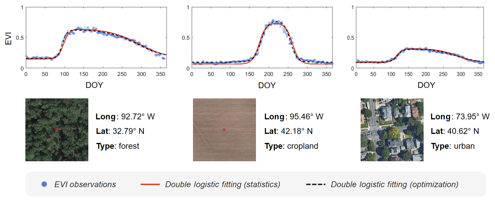
Figure 2Seasonal patterns of vegetation growth captured by the double logistic model for three distinctly different land cover types. The extent of a snapshot is 100 m × 100 m, and the red dot in the snapshot is the location of the enhanced vegetation index (EVI) plot. EVI observations were composited using all clear-sky pixels during the past 3 decades (1985–2015).
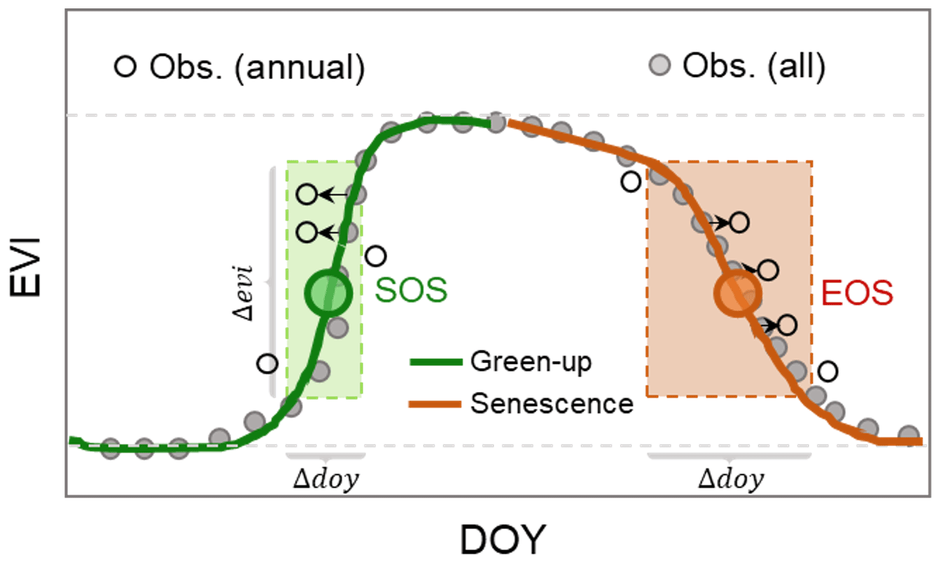
Figure 3Illustration of the generalized Landsat phenology (GLP) approach for identifying the annual variability of phenology indicators. The solid circles are long-term enhanced vegetation index (EVI) observations and the empty circles are observations at a specific year. The shaded frames colored as green and brown are the rational ranges of day of year (DOY) and EVI to be used during the green-up and senescence phases, respectively.
We characterized the seasonal change of vegetation growth using a double logistic model. This model has several advantages compared to other approaches such as the splines and harmonic models (Melaas et al., 2016b; Carrão et al., 2010): (1) it captures the green-up and senescence phases using different sigmoid functions, and (2) the physical meaning of parameters is related to the vegetation growth and senescence (Fisher et al., 2006; Li et al., 2017b). The derived EVI time series data were fitted using the double logistic model as Eq. (1).
where f(t) is the fitted EVI value at the day t; v1 and v2 are the background and amplitude of EVI over the entire year, respectively; and m1 & n1, m2 & n2 are the paired parameters that capture the trends of the green-up and senescence phases of vegetation growth, respectively. That is, n1 and n2 are dates with maximum increasing and decreasing rates of green-up and senescence in sigmoid curves, and m1 and m2 are the slopes that determine the shape of sigmoid curves.
We developed a stepwise statistical approach to estimate the parameters of the double logistic model on the GEE platform for large-scale applications because the GEE platform currently does not support the optimization of parameters. Calculation of these parameters was presented in the Appendix. In general, the performance of this GEE-based double logistic model is robust for different land cover types, and the derived results are close to that from the optimization algorithm (Fig. 2). For example, although the magnitude of EVIs is relatively low in urban areas with low vegetation cover, a distinctive seasonal pattern of vegetation growth can be captured by the double logistic model. Also, sigmoid curves during green-up and senescence phases are notably different across different vegetation cover types (e.g., forest and cropland). We evaluated the performance of the fitted double logistic model based on the correlation between the fitted and observed EVI observations. Pixels affected by land use/cover change during the study period or having weak vegetation signals (e.g., extremely high built-up area or barren land) could have a lower fitting performance (i.e., correlation coefficient), and these pixels can be excluded for specific applications. A more detailed explanation of this procedure is reported in Li et al. (2017b). This stepwise statistical approach can be implemented at the pixel level on the GEE platform in a parallel manner, which significantly improved our mapping efficiency at the large scale.
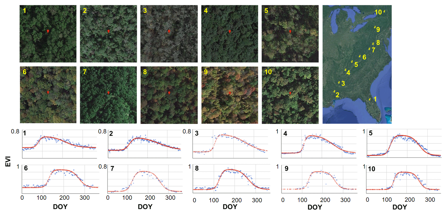
Figure 4Performance of the Google Earth Engine (GEE)-based double logistic model from the south to the north in the United States using forest as an example. Each snapshot indicates a 1 km2 square, and the red dot in the middle is the location (30 m) of the enhanced vegetation index (EVI) time series fitting.

Figure 5Performance of the Google Earth Engine (GEE)-based double logistic model for sites from the urban center to rural areas in the Chicago metropolitan area. Each snapshot indicates a 1 km2 square, and the red dot in the middle is the location (30 m) of the enhanced vegetation index (EVI) time series fitting.
We derived phenology indicators of SOS and EOS using a half-maximum criterion method (Fisher et al., 2006). In this method, SOS and EOS were calculated as the dates when the first derivative of EVI reaches the maximum increasing and decreasing rates during the green-up and senescence phases, respectively. Although there are other definitions of SOS and EOS, such as inflection points (i.e., at the base of sigmoid curve) (Zhang et al., 2003), the criterion used in our study is more temporally stable and can be applied to plants with different canopy structures (Fisher and Mustard, 2007). The growing season length (GSL) was defined as the difference between EOS and SOS.

Figure 6Comparison of the period (2001–2015) mean phenology indicators of the start of season (SOS) (a) and the end of season (EOS) (b) derived from Landsat and PhenoCam observations. COR: the correlation coefficient between the raw and fitted EVIs using the double logistic model.
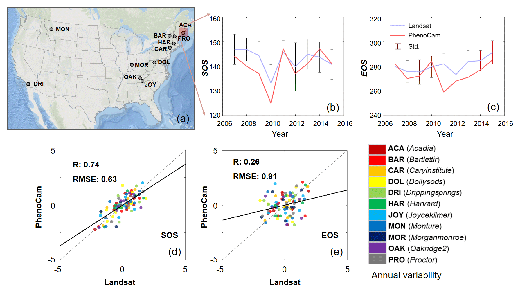
Figure 7Selected PhenoCam sites of deciduous broadleaf forest (a). Annual time series of phenology indicators in the station of Acadia for the start of season (SOS) (b) and the end of season (EOS) (c). Comparison of annual variability of SOS (d) and EOS (e) between Landsat and PhenoCam phenology indicators across all stations. The annual variability for each site is defined as , where x is the annual value of SOS and EOS and μ and σ are mean and standard deviation of SOS or EOS over the years.
3.2 Annual variability of phenology indicators
We derived the annual variability of vegetation phenology indicators using the developed generalized Landsat phenology (GLP) approach (Li et al., 2017b). Considering the temporally uneven distribution of available Landsat observations over the years, the annual variability of phenology indicators was measured as the difference of dates when the EVI in a specific year reaches the same magnitude as its long-term mean (Fisher et al., 2006; Melaas et al., 2013). Only EVI observations in the rational ranges of DOY and EVI (empty circles in shaded frames) in a given year were used in the GLP approach (Fig. 3). Observations outside this range (the shaded frames), which are either outliers or beyond the temporal ranges of the green-up and senescence phases, were not used in calculating the annual variability. In the GLP approach, we also designed a self-adjusting strategy to derive the bounds of the shaded frames in the green-up and senescence phases (Fig. 3). For the green-up phase, the rational DOY ranges (two points on the long-term mean curve that intersected with the shaded green frame in Fig. 3) were defined as the dates when change rates (or derivative) of EVI reach the half-maximum before and after the date of SOS (i.e., the date with the maximum change rate). Thus, the corresponding EVI ranges were calculated based on the derived DOY ranges and the long-term mean curve. The rational ranges of the senescence phase were determined using a similar approach. This approach already showed its applications for different vegetation types (e.g., cropland or forest) with varying seasonal patterns of EVI. More details about this approach can be found in Li et al. (2017b).
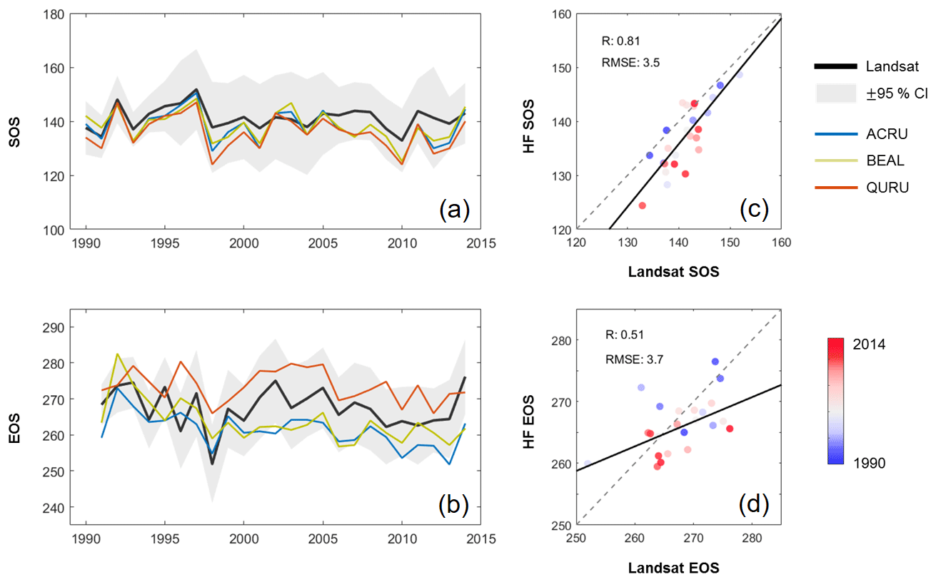
Figure 8Annual dynamics of the start of season (SOS) (a) and the end of season (EOS) (b) derived from Landsat and Harvard Forest (HF) observations and their scatter plots of SOS (c) and EOS (d) over the years.
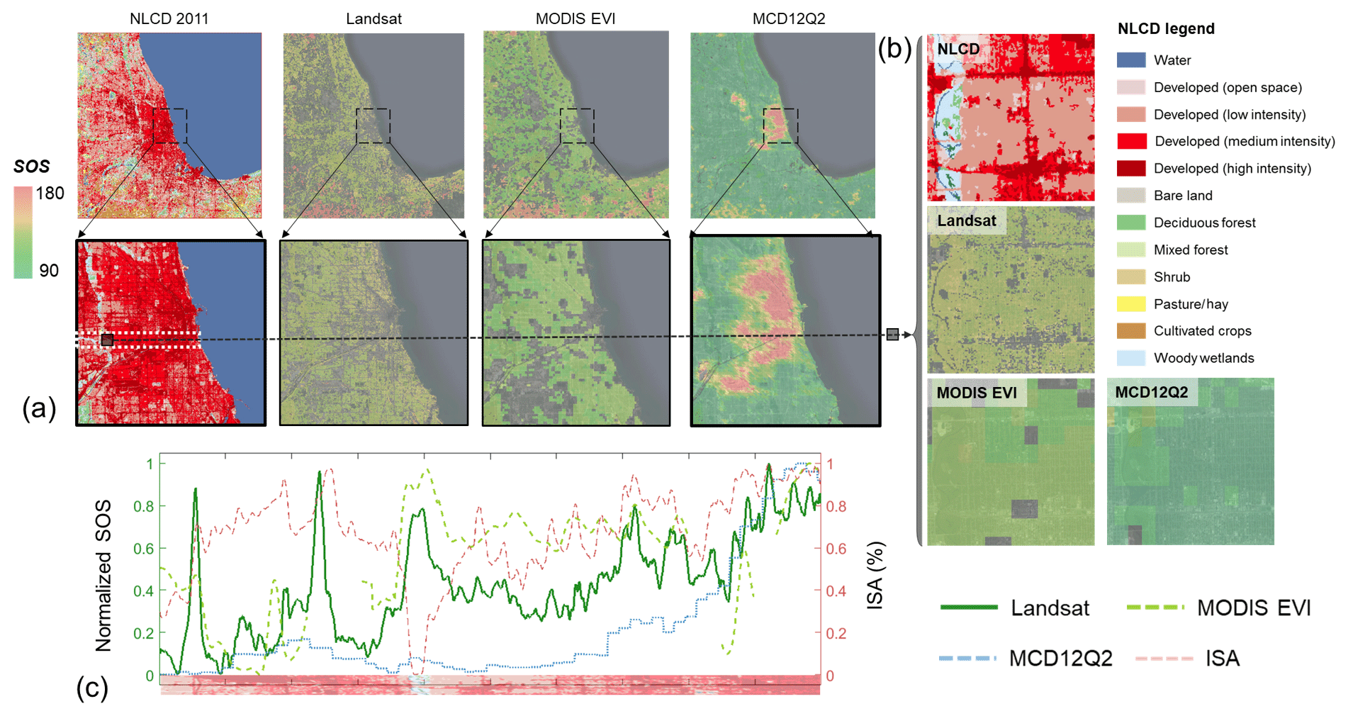
Figure 9Spatial patterns of the mean start of season (SOS) (2001–2014) derived from Landsat, the Moderate Resolution Imaging Spectroradiometer (MODIS) enhanced vegetation index (EVI), and MCD12Q2 and the land cover from the national land cover database (NLCD) (2011) in the Chicago metropolitan area (a). Enlarged views (b) at the location of the black square in (a). Change of normalized SOS and impervious surface area (ISA) (c) along the white rectangle in (a) (from left to right). Pixels without good fitting performance (i.e., the correlation coefficient is lower than 0.85) were removed in the derived SOS from Landsat and MODIS EVI.
4.1 Performance of the GEE-based double logistic model
The performance of the developed GEE-based double logistic model is reasonably good across different latitudes and different vegetation cover types in urban ecosystems. Take forest as an example, the seasonal pattern of EVI varies from the south to the north in the US, with notably different sigmoid curves for the green-up and senescence phases (Fig. 4). Our fitting approach can capture the diverse seasonal patterns of EVI for forest across space well. At the city scale, the proposed double logistic model shows a good performance for fitting EVI time series from urban to rural areas (Fig. 5), where the vegetation composition and the seasonal pattern of EVI are more complicated compared to natural ecosystems. For sites in the urban center, despite their low value of EVIs, a distinctive seasonal pattern of phenology is also captured by the proposed double logistic function with a good fitting performance.
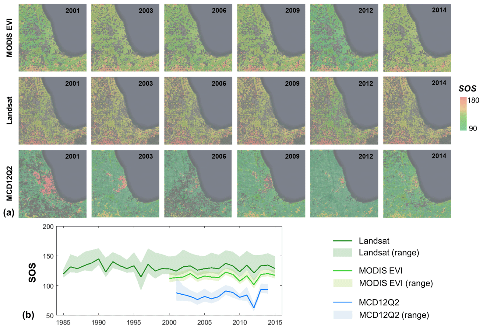
Figure 10Annual start of season (SOS) derived from Landsat, the Moderate Resolution Imaging Spectroradiometer (MODIS) enhanced vegetation index (EVI), and MCD12Q2 in the Chicago metropolitan area in representative years (a) and the temporal trend at the regional level (b). Solid lines are the mean SOSs at the regional level and shadowed frames indicate the range of SOS within the 25th and 75th quantile levels. Pixels without good fitting performance (i.e., the correlation coefficient is lower than 0.85) were removed in the derived SOS from Landsat and MODIS EVI.
4.2 Comparison with PhenoCam data
Overall, the derived phenology indicators (SOS and EOS) are spatially consistent with those from in situ PhenoCam data at the large (e.g., national) scale (Fig. 6). PhenoCam is a regional-scale network of digital cameras that provide high temporal resolution vegetation canopy and phenology information (Richardson et al., 2018). The records in PhenoCam are the observed green chromatic coordinate (GCC), which is used as the indicator of vegetation dynamics. We used all PhenoCam sites in the US and compared the mean SOS and EOS with Landsat-derived results. The definition of SOS and EOS we used in the PhenoCam data (i.e., the half-maximum criterion) is consistent with our result derived from Landsat data. Overall, correlations of the derived SOS and EOS from the Landsat and PhenoCam are 0.66 and 0.43, respectively. Most indicators are around the 1:1 line, indicating a close correspondence of phenology indicators derived from these two independent datasets. For those sites (blue or light-blue dots) with relatively large differences, the performance of fitting Landsat EVIs using the double logistic model is relatively low because these sites are mainly embedded in ecosystems that are dominated by shrubs, evergreen forests, or wetlands (Fig. S3). With correlation coefficients lower than 0.85 (worse fitting) excluded, as suggested by Melaas et al. (2016b), the overall agreements between Landsat- and PhenoCam-derived results were notably improved to 0.86 and 0.94, for SOS and EOS, respectively. Discrepancies between these two sets of phenology indicators derived from Landsat and PhenoCam are mainly attributed to factors such as (1) two different vegetation indices (i.e., EVI and GCC); and (2) the scale effect between in situ PhenoCam and Landsat observations (Liu et al., 2017).
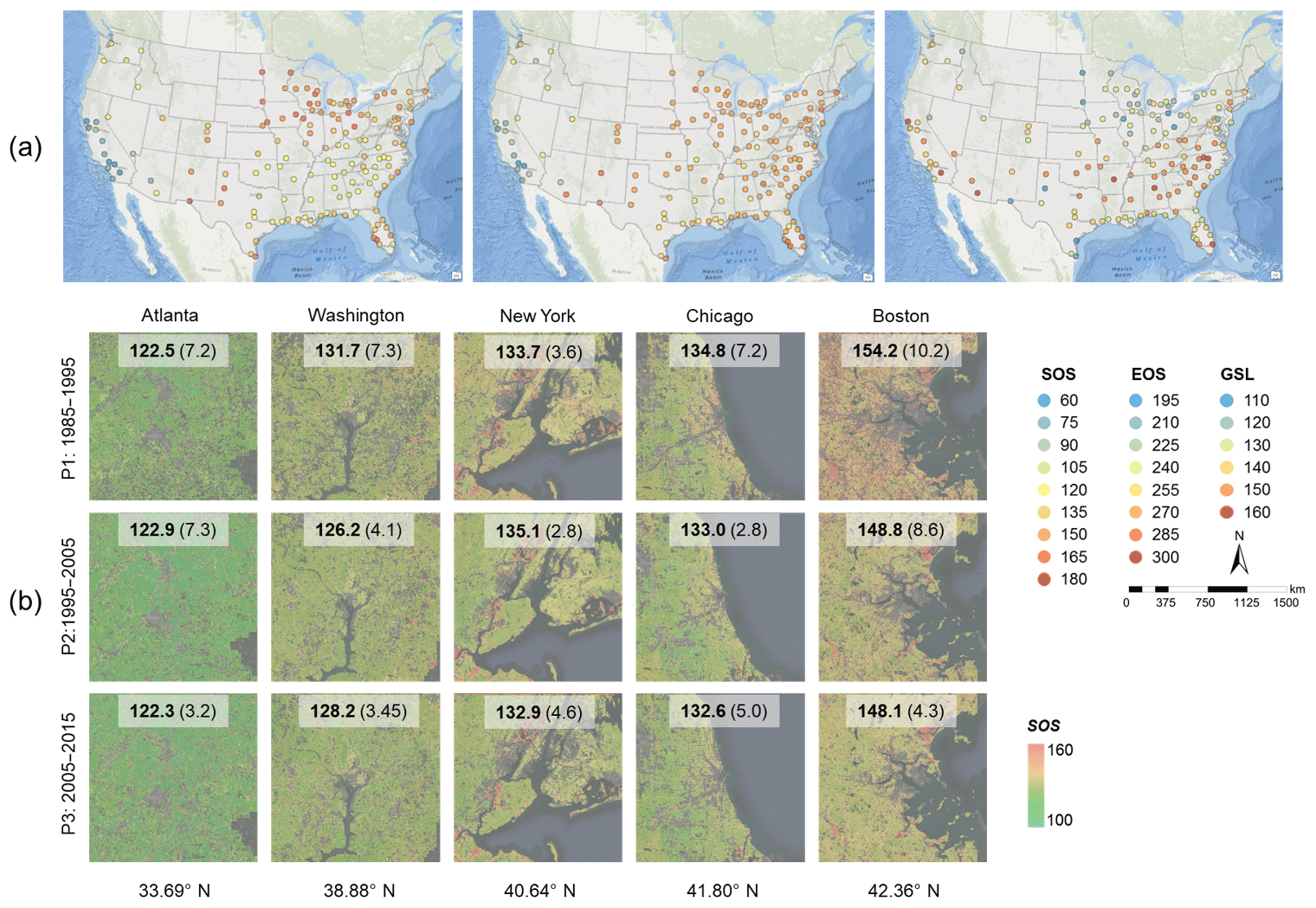
Figure 11Spatial patterns of the mean (1985–2015) vegetation phenology indicators (start of season, SOS, end of season, EOS, and growth season length, GSL) in American cities (a) and SOS in representative cities over the past 3 decades (b). Each dot in (a) represents the center of the urban cluster, and the spatial extent of selected cities in (b) is 25 km × 25 km. The mean SOS of each city and its standard deviation within each period (in parentheses) are provided in (b).
Overall, the annual variability of SOS derived from Landsat observations is consistent with that from the in situ PhenoCam observations (Fig. 7). We selected 11 deciduous broadleaf forest sites for comparison with continuous observations of more than 5 years (Fig. 7a). Landsat pixels located within 500 m of each PhenoCam station were used to ensure adequate samples to reflect the vegetation phenology dynamic at the local scale for this comparison (Melaas et al., 2016a). The temporal dynamics of Landsat-derived SOS and EOS generally follow the changes captured by PhenoCam observations (Fig. 7b–c). A detailed illustration of the Acadia site indicates the SOS derived from the two datasets is notably advanced during period 2006–2010 and their corresponding EOS is delayed after 2011. Although magnitudes of SOS and EOS are different over the years, their temporal trends (i.e., advanced or delayed) are relatively consistent. The magnitude differences of SOS from Landsat and MODIS are likely attributed to the scale effect, which determines different phenology patterns within a particular remotely sensed pixel. Overall, the annual SOS indicator derived from Landsat shows a better agreement (0.74) with the result obtained from in situ PhenoCam observations (Fig. 7d). The agreement of annual variability of Landsat and PhenoCam EOS is relatively weak (0.26) (Fig. 7e), which is consistent with previous results reported by Melaas et al. (2016a). The main reason for the weak agreement of annual variability of EOS is the difference in greening represented by GCC and EVI. That is, in the green-up phase, both GCC and EVI are rapidly increasing. While in the senescence phase, the EVI detected by Landsat slightly decreases, which is notably different from the pattern reflected by GCC that rapidly decreases once the leaf color changes.
4.3 Comparison with Harvard Forest phenology data
Our Landsat-derived phenology indicators have a similar temporal pattern with that from Harvard Forest (HF) over the past decades (Fig. 8). The HF data were collected by field observers in spring and fall seasons for more than 25 years (Richardson et al., 2006). Our Landsat-derived indicators were compared with dates of SOS and EOS recorded in the HF data, in which SOS and EOS are defined as the dates when the leaf length reaches 50 % of its final size and the leaf color reaches 10 % of the color change to the greenest, respectively (Melaas et al., 2016a). Three dominant species of deciduous forest in the HF, including red oak (Quercus rubra; QURU), red maple (Acer rubrum; ACRU), and yellow birch (Betula alleghaniensis; BEAL), were used in our analysis. However, for other vegetation types (e.g., evergreen forest), discernible phenology patterns can be also captured using the proposed methodology (e.g. Fig. 4, Site 1). Overall, the SOS of the three dominant species in the HF is similar and has a similar temporal trend with SOS derived from Landsat observations (Fig. 8a). The RMSE between Landsat SOS and the HF data is 3.5 d, and the correlation coefficient is 0.81 (Fig. 8c), indicating a comparable SOS and a relatively consistent temporal pattern. EOS shows a relatively large gap among species (Fig. 8b), i.e., the EOS of red oak is notably later compared to other two species of red maple and yellow birch. The Landsat-derived EOS is within the range of EOS of the three species, and the temporal variabilities of the two data sources are similar, although their magnitudes are different. The RMSE between Landsat EOS and the HF data is 3.7 d, and the correlation coefficient is 0.51 (Fig. 8d).
4.4 Comparison with MODIS data
Phenology indicators (e.g., SOS) derived from Landsat observations provide more spatial details in and around urban areas and are spatially consistent with those from MODIS (Fig. 9). Taking the Chicago metropolitan area as an example, we compared the Landsat-derived SOS with that from MODIS in two ways. First, we estimated SOS from the MODIS EVI (16 d) using the same approach for Landsat. Second, we retrieved SOS from the widely used MODIS phenology product (MCD12Q2) (Zhang et al., 2003) for comparison with Landsat-based SOS. It is worthy to note that the SOS defined in MCD12Q2 is the inflection point of EVI growth during the green-up phase, and this definition is different from our half-maximum criterion (Fisher and Mustard, 2007). Therefore, the SOS of MCD12Q2 is generally earlier than the other two. Also, there might be uncertainties in MCD12Q2 in highly urbanized regions with SOS above 180 d (Zhou et al., 2016) (Fig. 9a). Overall, more spatial details of SOS can be revealed in results derived from Landsat compared to MODIS (Fig. 9b). In highly urbanized regions, Landsat SOS can also capture the seasonal pattern of vegetation growth. Normalized SOSs derived from MODIS and Landsat show a relatively consistent trend along the gradient of developed areas (Fig. 9c), although their magnitudes are different (Fig. 9a).
Landsat-derived phenology indicator of SOS exhibits a consistent temporal pattern compared to MODIS with a longer temporal span (Fig. 10). Although the temporal distribution of Landsat is uneven compared to MODIS, the annual variability of phenology indicators can be captured well using the clear EVI observations in a given year relative to the long-term mean pattern. For example, there is a notable advancement of SOS in 2012, and all three SOSs capture this variability at the pixel and regional levels (Fig. 10a and b). The magnitude difference of derived SOS between Landsat and MCD12Q2 is mainly due to their definitions, and the difference of SOS between Landsat and MODIS EVI is likely caused by the scale effect (e.g., mixed pixels). It is worth noting that SOS derived from the half-maximum criterion in this study is consistently later when compared to the MODIS product using the criterion of the inflection point.
4.5 Spatiotemporal patterns of phenology indicators
Phenology indicators (SOS, EOS, and GSL) in urban domains exhibit a spatially explicit pattern from the north to the south in the conterminous US, with an overall advanced SOS in the past 3 decades (Fig. 11). SOS becomes earlier and EOS becomes later along the latitudinal gradient, although such spatial difference is more discernible in SOS compared to EOS at the national scale. As a result, GSL shows a generally extended trend from the north to the south (Fig. 11a). This spatial pattern of latitudinal change of phenology indicators (e.g., SOS) is also confirmed at the city level with more detail (Fig. 11b) and benefits from the higher spatial resolution of Landsat data. Meanwhile, the SOS in the last decade (P3: 2005–2015) is generally earlier than that in the first decade (P1: 1985–1995), although the temporal trend with an earlier SOS in the past 3 decades is not significant for all cities. The spatiotemporal patterns of phenology indicators in the conterminous US reflect the response of vegetation phenology to regional differences of elevation, temperature, precipitation, vegetation type, and global warming in past decades (Zhang et al., 2004a; Li et al., 2017a). In addition, changes in urban environments such as impervious surfaces, air pollution, and species compositions can affect the spatiotemporal pattern of vegetation phenology in urban ecosystems (Li et al., 2015; Escobedo et al., 2011).
The derived vegetation phenology data in urban domains are available at https://doi.org/10.6084/m9.figshare.7685645.v5 (Li et al., 2019a).
This study generated the first national-scale dynamics of annual vegetation phenology in urban domains (all urban areas greater than 500 km2 and their surrounding rural areas) using long-term (1985–2015) Landsat observations on the GEE platform. First, we mapped the long-term mean seasonal pattern of vegetation dynamics using a double logistic model. In this step, we proposed a stepwise statistical approach to estimate parameters in the double logistic model and implemented it on the GEE platform. Next, we identified annual dynamics of phenology indicators (i.e., SOS and EOS) by measuring the difference of dates when the EVI in a specific year reaches the same magnitude as its long-term mean. Finally, we developed the first medium spatial resolution (30 m) phenology product in urban areas in the conterminous US over the past 3 decades (1985–2015).
Overall, the Landsat-based phenology indicators agree with those derived from independent in situ observations (PhenoCam and HF) and another widely used satellite observations from MODIS. Overall, the phenology indicators derived from Landsat and PhenoCam are consistent for their long-term mean and annual variability. The comparison with field observations collected in the HF suggests the Landsat-derived indicators can capture the temporal dynamics of vegetation phenology in this forest ecosystem. Besides, the Landsat-derived phenology indicators can provide more spatial details in and around urban areas compared to the coarse-resolution MODIS results. Also, the temporal trends of the phenology indicator (e.g., SOS) derived from Landsat and MODIS are consistent overall, and Landsat additionally extends the temporal span of MODIS back to the past 3 decades.
The Landsat phenology product in urban areas is of great use in urban phenology studies such as phenology response to urbanization. There is a spatially explicit pattern of phenology indicators from the north to the south in US cities, with an overall advanced SOS in the past 3 decades. With this new phenology dataset (i.e., a long temporal coverage and a medium spatial resolution), the response of vegetation phenology to urbanization (e.g., UHI) can be further investigated, particularly for plants in the urban center or suburban areas with urban environment that have been notably altered by anthropogenic activities, where most people reside (Zhang et al., 2004b; Alberti et al., 2017). This dataset, together with ground-based pollen concentration data, is also of help in decision making relevant to pollen-induced allergy diseases (Li et al., 2019b). In addition, the derived leaf on and off information in this dataset is potentially useful for many vegetation–air pollution deposition models (Escobedo and Nowak, 2009). However, it is worth noting that this dataset is most applicable for deciduous forest type. For grassland and evergreen forests in tropical areas, the uncertainty could be high in the derived phenology indicators. In addition, our phenology algorithm did not specifically consider pixels with land cover changes, which could be further improved when the product of annual urban dynamics becomes available.
The double logistic model used in the GLP approach includes two sigmoid curves indicating the green-up and senescence phases of vegetation growth (Eq. A1).
where f(t) is the fitted EVI value at the day t; v1 and v2 are the background and amplitude of EVI over the entire year, respectively; the first sigmoid ( with pair-parameters of m1 and n1 captures the green-up phase of vegetation growth; and the second sigmoid ( with pair-parameters of m2 and n2 captures the senescence phase of vegetation growth (Fig. A1).
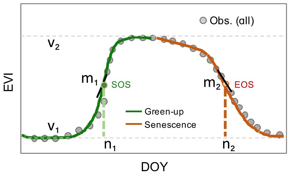
Figure A1Illustration of the double logistic model and corresponding parameters. EVI: enhanced vegetation index; DOY: day of year.
We derived six parameters (i.e., v1, v2, m1, n1, m2, and n2) in the double logistic model using a statistics approach on the GEE platform. First, we estimated v1 and v2 based on the smoothed EVI time series, with abnormal observations (or noise) excluded. We calculated the quantile levels of 5th and 95th as the minimum v1 and maximum EVI vmax over the entire DOY range to avoid possible biases caused by extreme values. Thus, v2 can be determined with Eq. (A2).
The first part (Sig1) of the double logistic model in the green-up phase (Eq. A3) can be translated to Eq. (A4) by using the smoothed EVI time series only during the green-up phase before doymax and converted into a logarithmic form as Eq. (A5).
where the left term in Eq. (A5) can be calculated using v1 and v2, together with the smoothed EVI time series f(t) only during the green-up phase before doymax. m1 and n1 can be estimated using the least-squares-regression approach.
Finally, based on the estimated parameters (i.e., v1, v2, m1 and n1), the second part (Sig2) of the double logistic model in the senescence phase can be formulated as Eqs. (A6)–(A8), respectively. In a similar manner, the pair-parameters of m2 and n2 can be estimated using the least-squares-regression approach together with the smoothed EVI time series during the green-up and senescence phases.
The supplement related to this article is available online at: https://doi.org/10.5194/essd-11-881-2019-supplement.
YZ and XL designed the research; XL and YZ implemented the research and wrote the paper; GRA, LM, CL, and QW edited and revised the manuscript.
The authors declare that they have no conflict of interest.
We acknowledge funding support from the NASA ROSES INCA Program (NNH14ZDA001N-INCA). We would like to thank organizations that shared their datasets for use in this study, and the two reviewers and the handling editor for their constructive comments and suggestions.
This research has been supported by the NASA ROSES INCA (grant no. NNH14ZDA001N-INCA).
The article processing charges for this open-access
publication were covered by the Iowa State University Library.
This paper was edited by David Carlson and reviewed by Yongshuo Fu and Francisco J. Escobedo.
Aas, K., Aberg, N., Bachert, C., Bergmann, K., Bergmann, R., and Bonini, S.: Allergic disease as a public health problem in Europe, European allergy white paper, Brussel: UCB Insitute of Allergy, 1–46, 1997.
Alberti, M., Correa, C., Marzluff, J. M., Hendry, A. P., Palkovacs, E. P., Gotanda, K. M., Hunt, V. M., Apgar, T. M., and Zhou, Y.: Global urban signatures of phenotypic change in animal and plant populations, P. Natl. Acad. Sci. USA, 114, 8951–8956, https://doi.org/10.1073/pnas.1606034114, 2017.
Anenberg, S. C., Weinberger, K. R., Roman, H., Neumann, J. E., Crimmins, A., Fann, N., Martinich, J., and Kinney, P. L.: Impacts of oak pollen on allergic asthma in the United States and potential influence of future climate change, GeoHealth, 1, 80–92, 2017.
Carrão, H., Gonçalves, P., and Caetano, M.: A nonlinear harmonic model for fitting satellite image time series: Analysis and prediction of land cover dynamics, IEEE Trans. Geosci. Remote Sens., 48, 1919–1930, 2010.
Cong, N., Piao, S., Chen, A., Wang, X., Lin, X., Chen, S., Han, S., Zhou, G., and Zhang, X.: Spring vegetation green-up date in China inferred from SPOT NDVI data: A multiple model analysis, Agr. Forest Meteorol., 165, 104–113, https://doi.org/10.1016/j.agrformet.2012.06.009, 2012.
Escobedo, F. J. and Nowak, D. J.: Spatial heterogeneity and air pollution removal by an urban forest, Landscape Urban Plan, 90, 102–110, 2009.
Escobedo, F. J., Kroeger, T., and Wagner, J. E.: Urban forests and pollution mitigation: Analyzing ecosystem services and disservices, Environ. Pollut., 159, 2078–2087, 2011.
Fisher, J. I. and Mustard, J. F.: Cross-scalar satellite phenology from ground, Landsat, and MODIS data, Remote Sens. Environ., 109, 261–273, https://doi.org/10.1016/j.rse.2007.01.004, 2007.
Fisher, J. I., Mustard, J. F., and Vadeboncoeur, M. A.: Green leaf phenology at Landsat resolution: Scaling from the field to the satellite, Remote Sens. Environ., 100, 265–279, https://doi.org/10.1016/j.rse.2005.10.022, 2006.
Gong, P., Liang, S., Carlton, E. J., Jiang, Q., Wu, J., Wang, L., and Remais, J. V.: Urbanisation and health in China, Lancet, 379, 843–852, https://doi.org/10.1016/S0140-6736(11)61878-3, 2012.
Gorelick, N., Hancher, M., Dixon, M., Ilyushchenko, S., Thau, D., and Moore, R.: Google Earth Engine: Planetary-scale geospatial analysis for everyone, Remote Sens. Environ., 202, 18–27, https://doi.org/10.1016/j.rse.2017.06.031, 2017.
Hansen, M. C., Potapov, P. V., Moore, R., Hancher, M., Turubanova, S. A., Tyukavina, A., Thau, D., Stehman, S. V., Goetz, S. J., Loveland, T. R., Kommareddy, A., Egorov, A., Chini, L., Justice, C. O., and Townshend, J. R. G.: High-Resolution Global Maps of 21st-Century Forest Cover Change, Science, 342, 850–853, https://doi.org/10.1126/science.1244693, 2013.
Hogda, K. A., Karlsen, S. R., Solheim, I., Tommervik, H., and Ramfjord, H.: The start dates of birch pollen seasons in Fennoscandia studied by NOAA AVHRR NDVI data, Geoscience and Remote Sensing Symposium, 2002, IGARSS'02, 2002 IEEE International, 3299–3301, 2002.
Huete, A., Didan, K., Miura, T., Rodriguez, E. P., Gao, X., and Ferreira, L. G.: Overview of the radiometric and biophysical performance of the MODIS vegetation indices, Remote Sens. Environ., 83, 195–213, https://doi.org/10.1016/S0034-4257(02)00096-2, 2002.
Jochner, S. and Menzel, A.: Urban phenological studies – Past, present, future, Environ. Pollut., 203, 250–261, https://doi.org/10.1016/j.envpol.2015.01.003, 2015.
Jochner, S. C., Sparks, T. H., Estrella, N., and Menzel, A.: The influence of altitude and urbanisation on trends and mean dates in phenology (1980–2009), Int. J. Biometeorol., 56, 387–394, https://doi.org/10.1007/s00484-011-0444-3, 2011.
Keenan, T. F., Gray, J., Friedl, M. A., Toomey, M., Bohrer, G., Hollinger, D. Y., Munger, J. W., O/'Keefe, J., Schmid, H. P., Wing, I. S., Yang, B., and Richardson, A. D.: Net carbon uptake has increased through warming-induced changes in temperate forest phenology, Nat. Clim. Change, 4, 598–604, https://doi.org/10.1038/nclimate2253, 2014.
Li, X., Gong, P., and Liang, L.: A 30-year (1984–2013) record of annual urban dynamics of Beijing City derived from Landsat data, Remote Sens. Environ., 166, 78–90, https://doi.org/10.1016/j.rse.2015.06.007, 2015.
Li, X., Zhou, Y., Asrar, G. R., Mao, J., Li, X., and Li, W.: Response of vegetation phenology to urbanization in the conterminous United States, Global Change Biol., 23, 6030–6046, https://doi.org/10.1111/gcb.13562, 2017a.
Li, X., Zhou, Y., Asrar, G. R., and Meng, L.: Characterizing spatiotemporal dynamics in phenology of urban ecosystems based on Landsat data, Sci. Total Environ., 605–606, 721–734, https://doi.org/10.1016/j.scitotenv.2017.06.245, 2017b.
Li, X., Zhou, Y., Meng, L., Asrar, G., Lu, C., and Wu, Q.: A dataset of 30-meter annual vegetation phenology indicators (1985–2015) in urban areas of the conterminous United States, https://doi.org/10.6084/m9.figshare.7685645.v5, 2019a.
Li, X., Zhou, Y., Meng, L., Asrar, G. R., Sapkota, A., and Coates, F.: Characterizing the relationship between satellite phenology and pollen season: a case study of birch, Remote Sens. Environ., 222, 257–274, https://doi.org/10.1016/j.rse.2018.12.036, 2019b.
Liu, Y., Wu, C., Peng, D., Xu, S., Gonsamo, A., Jassal, R. S., Altaf Arain, M., Lu, L., Fang, B., and Chen, J. M.: Improved modeling of land surface phenology using MODIS land surface reflectance and temperature at evergreen needleleaf forests of central North America, Remote Sens. Environ., 176, 152–162, https://doi.org/10.1016/j.rse.2016.01.021, 2016.
Liu, Y., Hill, M. J., Zhang, X., Wang, Z., Richardson, A. D., Hufkens, K., Filippa, G., Baldocchi, D. D., Ma, S., Verfaillie, J., and Schaaf, C. B.: Using data from Landsat, MODIS, VIIRS and PhenoCams to monitor the phenology of California oak/grass savanna and open grassland across spatial scales, Agr. Forest Meteorol., 237–238, 311–325, https://doi.org/10.1016/j.agrformet.2017.02.026, 2017.
Luz de la Maza, C., Hernández, J., Bown, H., Rodríguez, M., and Escobedo, F.: Vegetation diversity in the Santiago de Chile urban ecosystem, Arbor. J., 26, 347–357, 2002.
Masek, J. G., Vermote, E. F., Saleous, N. E., Wolfe, R., Hall, F. G., Huemmrich, K. F., Gao, F., Kutler, J., and Lim, T.-K.: A Landsat surface reflectance dataset for North America, 1990–2000, Geosci. Remote Sens. Lett. IEEE, 3, 68–72, 2006.
Melaas, E. K., Friedl, M. A., and Zhu, Z.: Detecting interannual variation in deciduous broadleaf forest phenology using Landsat TM/ETM + data, Remote Sens. Environ., 132, 176–185, https://doi.org/10.1016/j.rse.2013.01.011, 2013.
Melaas, E. K., Sulla-Menashe, D., Gray, J. M., Black, T. A., Morin, T. H., Richardson, A. D., and Friedl, M. A.: Multisite analysis of land surface phenology in North American temperate and boreal deciduous forests from Landsat, Remote Sens. Environ., 186, 452–464, https://doi.org/10.1016/j.rse.2016.09.014, 2016a.
Melaas, E. K., Wang, J. A., Miller, D. L., and Friedl, M. A.: Interactions between urban vegetation and surface urban heat islands: a case study in the Boston metropolitan region, Environ. Res. Lett., 11, 054020, https://doi.org/10.1088/1748-9326/11/5/054020, 2016b.
Moody, A. and Johnson, D. M.: Land-surface phenologies from AVHRR using the discrete Fourier transform, Remote Sens. Environ., 75, 305–323, 2001.
Pekel, J.-F., Cottam, A., Gorelick, N., and Belward, A. S.: High-resolution mapping of global surface water and its long-term changes, Nature, 540, 418–422, https://doi.org/10.1038/nature20584, 2016.
Peng, S., Piao, S., Ciais, P., Myneni, R. B., Chen, A., Chevallier, F., Dolman, A. J., Janssens, I. A., Penuelas, J., Zhang, G., Vicca, S., Wan, S., Wang, S., and Zeng, H.: Asymmetric effects of daytime and night-time warming on Northern Hemisphere vegetation, Nature, 501, 88–92, https://doi.org/10.1038/nature12434, 2013.
Piao, S., Fang, J., Zhou, L., Ciais, P., and Zhu, B.: Variations in satellite-derived phenology in China's temperate vegetation, Global Change Biol., 12, 672–685, https://doi.org/10.1111/j.1365-2486.2006.01123.x, 2006.
Richardson, A. D., Bailey, A. S., Denny, E. G., Martin, C. W., and O'KEEFE, J.: Phenology of a northern hardwood forest canopy, Global Change Biol., 12, 1174–1188, 2006.
Richardson, A. D., Hufkens, K., Milliman, T., Aubrecht, D. M., Chen, M., Gray, J. M., Johnston, M. R., Keenan, T. F., Klosterman, S. T., and Kosmala, M.: Tracking vegetation phenology across diverse North American biomes using PhenoCam imagery, Sci. Data, 5, 180028, https://doi.org/10.1038/sdata.2018.28, 2018.
Tang, J., Körner, C., Muraoka, H., Piao, S., Shen, M., Thackeray, S. J., and Yang, X.: Emerging opportunities and challenges in phenology: a review, Ecosphere, 7, 1–17, https://doi.org/10.1002/ecs2.1436, 2016.
United Nations (Department of Economic and Social Affairs, Population Division): World Urbanization Prospects: The 2018 Revision, Highlights (ST/ESA/SER.A/352), 2018.
Walker, J. J., de Beurs, K. M., Wynne, R. H., and Gao, F.: Evaluation of Landsat and MODIS data fusion products for analysis of dryland forest phenology, Remote Sens. Environ., 117, 381–393, https://doi.org/10.1016/j.rse.2011.10.014, 2012.
Walker, J. J., de Beurs, K. M., and Henebry, G. M.: Land surface phenology along urban to rural gradients in the U.S. Great Plains, Remote Sens. Environ., 165, 42–52, https://doi.org/10.1016/j.rse.2015.04.019, 2015.
White, A. M., Nemani, R. R., Thornton, E. P., and Running, W. S.: Satellite Evidence of Phenological Differences Between Urbanized and Rural Areas of the Eastern United States Deciduous Broadleaf Forest, Ecosystems, 5, 260–273, https://doi.org/10.1007/s10021-001-0070-8, 2002.
Xiong, J., Thenkabail, P., Tilton, J., Gumma, M., Teluguntla, P., Oliphant, A., Congalton, R., Yadav, K., and Gorelick, N.: Nominal 30-m Cropland Extent Map of Continental Africa by Integrating Pixel-Based and Object-Based Algorithms Using Sentinel-2 and Landsat-8 Data on Google Earth Engine, Remote Sens., 9, 1065, https://doi.org/10.3390/rs9101065, 2017.
Zhang, X., Friedl, M. A., Schaaf, C. B., Strahler, A. H., Hodges, J. C. F., Gao, F., Reed, B. C., and Huete, A.: Monitoring vegetation phenology using MODIS, Remote Sens. Environ., 84, 471–475, https://doi.org/10.1016/S0034-4257(02)00135-9, 2003.
Zhang, X., Friedl, M. A., Schaaf, C. B., and Strahler, A. H.: Climate controls on vegetation phenological patterns in northern mid-and high latitudes inferred from MODIS data, Global Change Biol., 10, 1133–1145, 2004a.
Zhang, X., Friedl, M. A., Schaaf, C. B., Strahler, A. H., and Schneider, A.: The footprint of urban climates on vegetation phenology, Geophys. Res. Lett., 31, L12209, https://doi.org/10.1029/2004GL020137, 2004b.
Zhou, D., Zhao, S., Zhang, L., and Liu, S.: Remotely sensed assessment of urbanization effects on vegetation phenology in China's 32 major cities, Remote Sens. Environ., 176, 272–281, https://doi.org/10.1016/j.rse.2016.02.010, 2016.
Zhou, Y., Smith, S. J., Elvidge, C. D., Zhao, K., Thomson, A., and Imhoff, M.: A cluster-based method to map urban area from DMSP/OLS nightlights, Remote Sens. Environ., 147, 173–185, https://doi.org/10.1016/j.rse.2014.03.004, 2014.
Zhou, Y., Li, X., Asrar, G. R., Smith, S. J., and Imhoff, M.: A global record of annual urban dynamics (1992–2013) from nighttime lights, Remote Sens. Environ., 219, 206–220, 2018.
Zhu, Z. and Woodcock, C. E.: Object-based cloud and cloud shadow detection in Landsat imagery, Remote Sens. Environ., 118, 83–94, https://doi.org/10.1016/j.rse.2011.10.028, 2012.
Zipper, S. C., Schatz, J., Singh, A., Kucharik, C. J., Townsend, P. A., and Loheide, I., and Steven, P.: Urban heat island impacts on plant phenology: intra-urban variability and response to land cover, Environ. Res. Lett., 11, 054023, https://doi.org/10.1088/1748-9326/11/5/054023, 2016.