the Creative Commons Attribution 4.0 License.
the Creative Commons Attribution 4.0 License.
 | 05 Jul 2019
Environmental parameters of shallow water habitats in the SW Baltic Sea
Christian Lieberum
Gesche Bock
Rolf Karez
The coastal waters of the Baltic Sea are subject to high variations in environmental conditions, triggered by natural and anthropogenic causes. Thus, in situ measurements of water parameters can be strategic for our understanding of the dynamics in shallow water habitats. In this study we present the results of a monitoring program at low water depths (1–2.5 m), covering 13 stations along the Baltic coast of Schleswig-Holstein, Germany. The provided dataset consists of records for dissolved inorganic nutrient concentrations taken twice a month and continuous readings at 10 min intervals for temperature, salinity and oxygen content. Data underwent quality control procedures and were flagged. On average, a data availability of >90 % was reached for the monitoring period within 2016–2018. The obtained monitoring data reveal great temporal and spatial variabilities of key environmental factors for shallow water habitats in the southwestern Baltic Sea. Therefore the presented information could serve as realistic key data for experimental manipulations of environmental parameters as well as for the development of oceanographic, biogeochemical or ecological models. The data associated with this article can be found at https://doi.org/10.1594/PANGAEA.895257 (Franz et al., 2018).


Coastal areas represent highly variable environments. The proximity to land, shallow water depths and the direct influence of river discharges affect oceanography, biology and meteorology of these regions (Sinex, 1994). Drastic changes in water parameters like temperature, oxygen level or pH can occur within hours and minutes, often only detected at local spatial scales (Bates et al., 2018). Marine organisms experiencing these conditions exhibit different strategies to cope with those circumstances. In the context of studies on global change such consideration is crucial since biological communities are not directly affected by climate itself, but rather by shorter-term variabilities in environmental conditions (i.e., weather) (Helmuth et al., 2014). However, scientists are still widely applying large-scale averages (temporal and spatial) in experimental approaches, risking misleading interpretations in an either too positive or too negative direction (Bates et al., 2018). This might be the result of not only misconception, but also limited availability and accessibility of necessary information. Until today, the descriptions of monitoring programs designed for pure data acquisition are commonly published in grey literature and the respective data are not publicly available. The fact that many locations are facing extreme events that are far beyond average conditions projected for the future (e.g., Mills et al., 2013) underlines the urgent need for fine-scale data. Identifying and describing environmental variabilities (e.g., extreme events) would be a first step towards better predictions of climate change impacts.
The Baltic Sea is a particular example for environmental variability of natural and anthropogenic origin. It exhibits gradients of critical environmental drivers caused by its semi-enclosed characteristics and the large drainage area of surrounding landmasses, mainly reflected in decreasing salinity and temperature towards the north (Snoeijs-Leijonmalm et al., 2017). The major contribution to environmental variability caused by human activities in the Baltic Sea is represented by eutrophication. Nutrient concentrations rose until the mid-1980s by riverine inputs of nitrate and phosphate (HELCOM, 2018). The resulting enhanced primary productivity led to an increase in organic matter deposition, which fueled respiration at the seafloor and created hypoxic or even anoxic areas of great spatial extent (HELCOM, 2018). Even though nutrient inputs decreased in the last 2 decades, so-called “dead zones” are persisting, not least because climate warming is boosting deoxygenation (Carstensen et al., 2014). Consequently, shallow areas at the shore can experience episodic hypoxia resulting from oxygen-depleted bottom waters and, in addition, upwelling events that transport water from deeper basins to coastal areas (Conley et al., 2011; Saderne et al., 2013). In the latter case, benthic communities living in these habitats will face not just one but a set of environmental shifts: in addition to low oxygen levels, organisms are subjected to increased nutrient concentrations, lower temperatures, higher salinities and elevated pCO2 levels (Lehmann and Myrberg, 2008; Saderne et al., 2013). However, the impact of upwelling events on benthic communities is not straightforward, as the lower temperatures and higher salinities represent short-term relaxations from climate-driven warming and desalination predicted for the Baltic Sea (Jonsson et al., 2018).
The interacting influence of large- and local-scale gradients in water parameters leads to a pronounced variability in environmental conditions of coastal ecosystems in the Baltic Sea. To further develop our understanding of the dynamics communities are experiencing in shallow waters, a monitoring of water parameters along the Baltic coast of Schleswig-Holstein (Germany) was designed. In this contribution we are presenting the obtained data for water temperature, salinity, dissolved oxygen content and nutrient concentrations recorded within the period of 2016–2018.
2.1 Study area
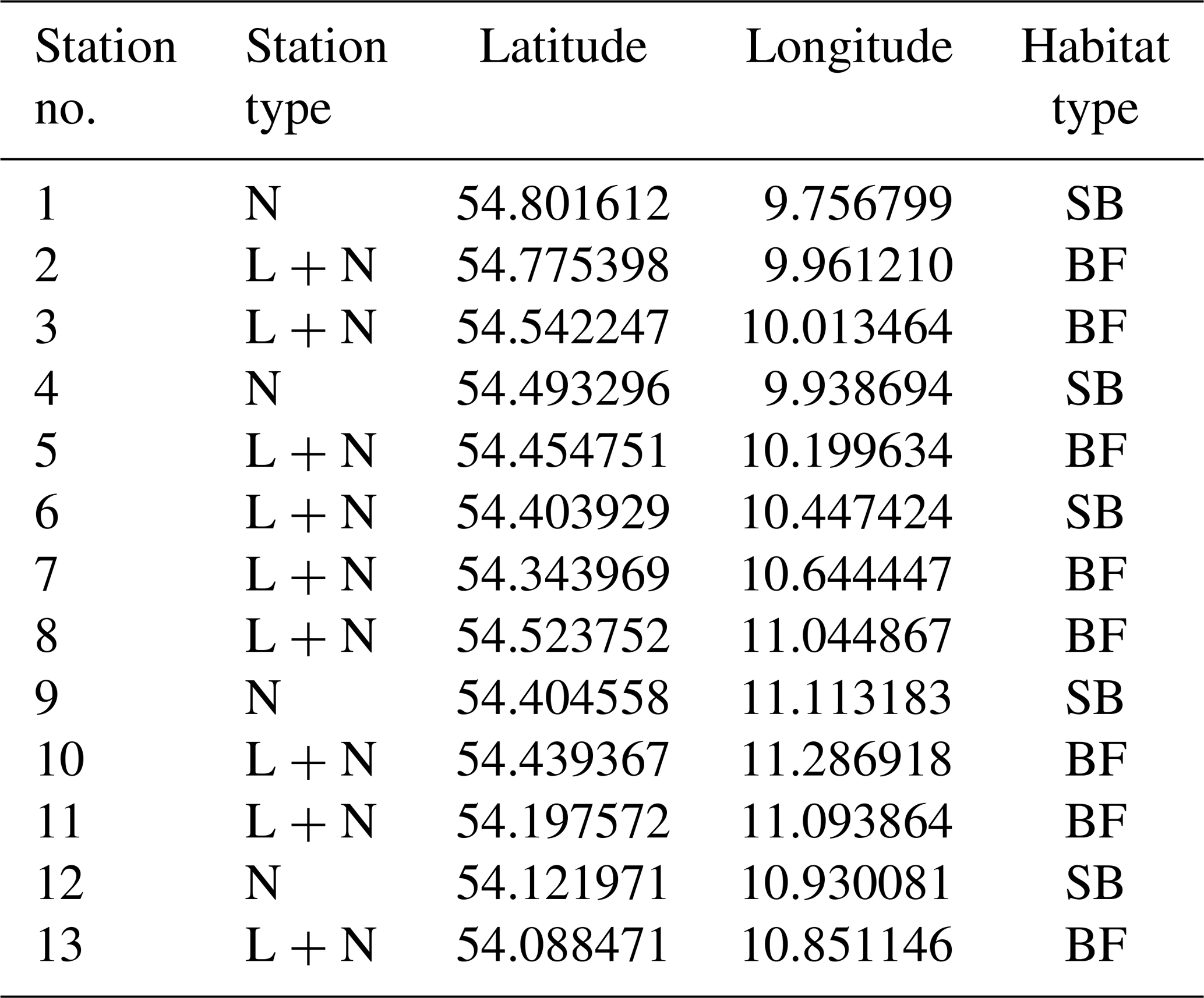
The monitoring sites are located along the Baltic Sea coast of Schleswig-Holstein, Germany. A total of 13 stations were established, with samplings for dissolved inorganic nutrient concentrations every 2 weeks at all stations and continuous recordings of environmental parameters (temperature, salinity and dissolved oxygen) at nine stations (Fig. 1). The stations are located in boulder field or sandy bottom habitats (Table 1).
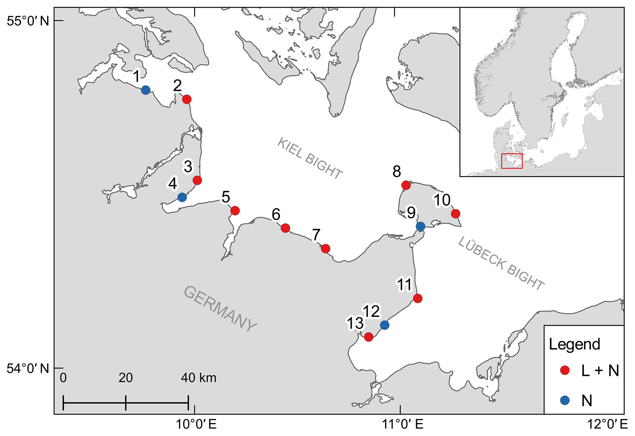
Figure 1Geographical position of the 13 monitoring stations. Colors indicate if only samples for dissolved inorganic nutrients were taken (N) or if a logger station was also deployed (L + N).
Table 1Characteristics of the sampling stations in the monitoring program. Station type depicts if only samples for dissolved inorganic nutrients were taken (N) or if in addition continuous recordings by data-loggers (L + N) were performed. Codes for habitat type are as follows. BF: boulder field; SB: sandy bottom.
2.2 Nutrient sampling and analysis
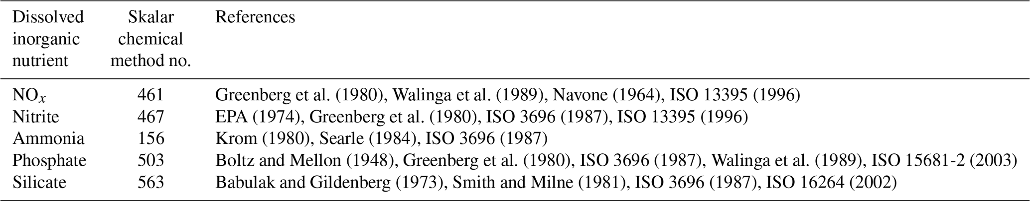
Twice per month water samples were collected from a water depth of 1 m at all stations. Two water samples were collected at each station per sampling event. In the sampling routine, Stations 1–7 were always sampled in the same week and Stations 8–13 in the following week. Wearing a chest wader, the person collecting the water sample walked until reaching the sampling station at a water depth of approximately 1.2 m. In the case of stations equipped with a logger station (see Sect. 2.3), the water sample was collected leaving the shore line in a roughly perpendicular direction heading towards the logger station until reaching the desired water depth of approximately 1.2 m. Water samples were collected using a 50 mL syringe connected to a plastic tube of 1 m length. For sampling, the syringe was held at the water surface and the tube was lowered to 1 m depth. Care was taken not to suck sediment from the sea floor. All sampling equipment (syringe, tube, scintillation vials) was rinsed with water from the collection site before the actual sample was taken. Immediately after the water was collected with the syringe, it was filtered using a cellulose acetate syringe filter (0.45 µm) while filling the sample into a scintillation vial. Back in the laboratory, the samples were directly put into a freezer and kept at −20 ∘C until further sample processing. Subsequently, the samples were analyzed for the concentration of dissolved inorganic nutrients (total oxidized nitrogen, nitrite, ammonia, phosphate and silicate) by UV–vis spectroscopy using a continuous-flow analyzer (San Automated Wet Chemistry Analyzer, Skalar Analytical B.V.). For the analyses, chemical methods provided by Skalar were applied (Table 2). Total oxidized nitrogen concentrations (NOx) were determined by the cadmium reduction method, followed by measurement of nitrite (originally present plus reduced nitrite).
Table 2Chemical methods applied to measure dissolved inorganic nutrient concentrations in the water samples. NOx: total oxidized nitrogen.
2.3 Data logger setup
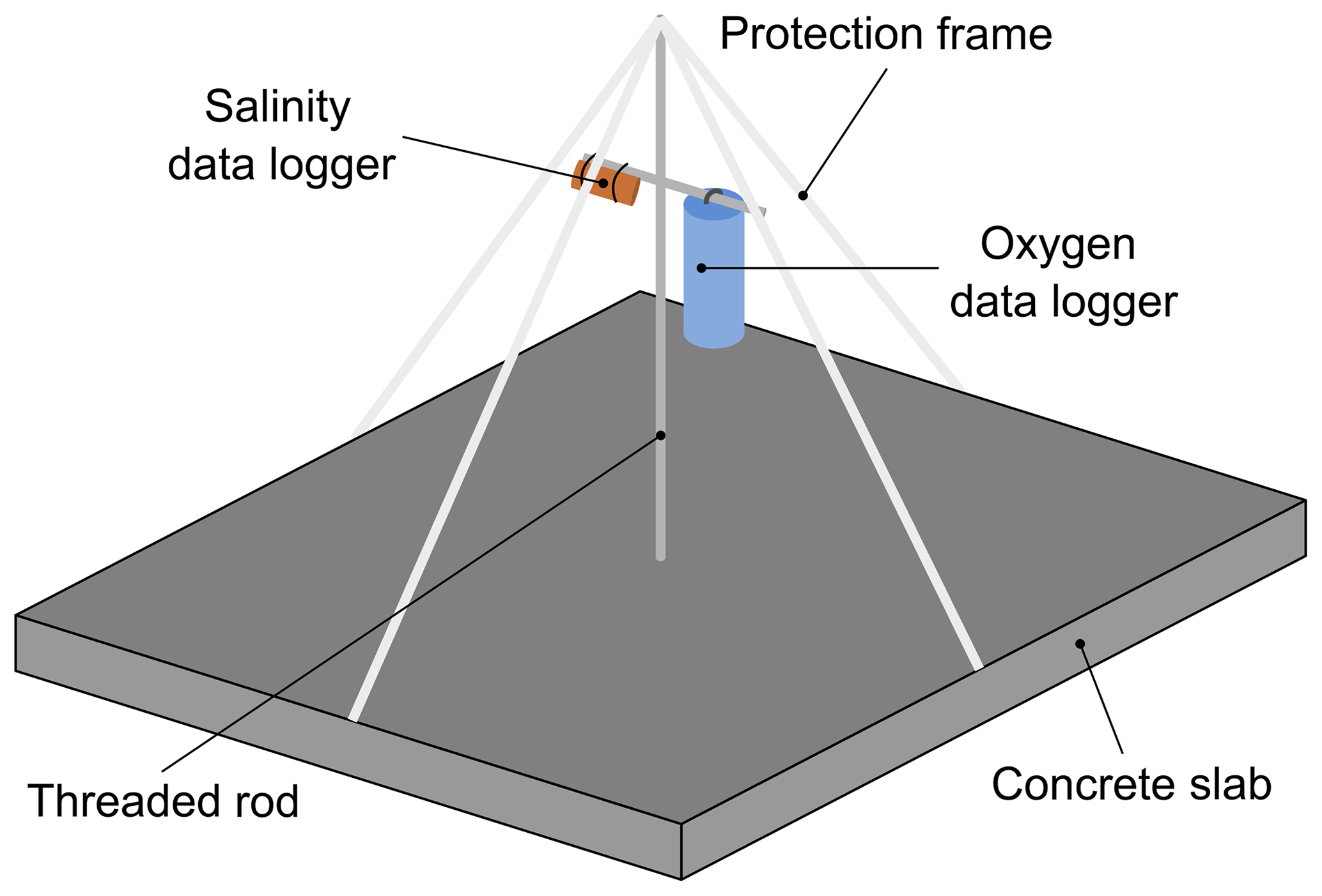
Nine logger stations were deployed in the field at a depth of 2.5 m to continuously record data for temperature, salinity and dissolved oxygen. Each logger station consisted of a concrete slab (50 cm ×50 cm) equipped with a vertical threaded stainless-steel bar, which was used as a mounting structure for data loggers (Fig. 2). The data loggers were fixed at the threaded stainless-steel bar 40 cm above the seafloor. To protect the sensors from fishing gear and drifting material, a frame was constructed around the setup by connecting plastic tubes to the end of the metal rod and to each side of the concrete slab.
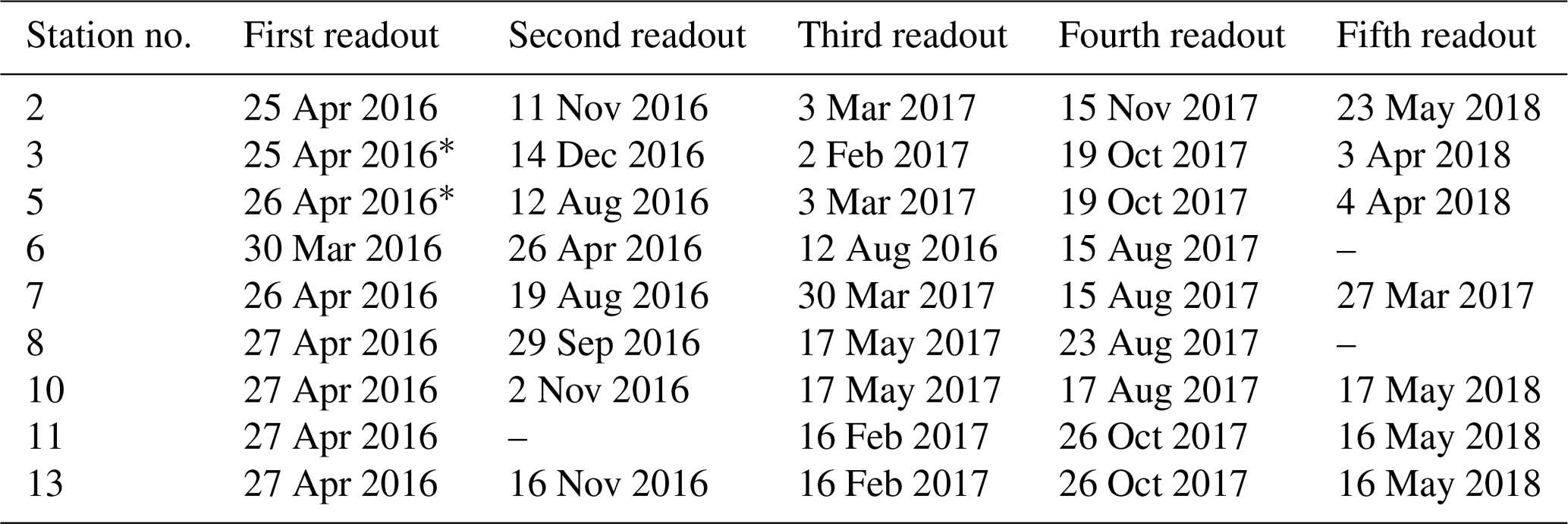
Two types of self-contained data loggers were used for the logger stations: (I) MiniDOT loggers (Precision Measurement Engineering; https://www.pme.com/, last access: 1 July 2019; ±10 µmol L−1 or ±5 % saturation) including an antifouling copper option (copper plate and mesh) to measure dissolved oxygen concentration and (II) DST CT salinity & temperature loggers (Star-Oddi; https://www.star-oddi.com/, last access: 1 July 2019; ±1.5 mS cm−1) recorded the conductivity. Both sensors additionally recorded water temperature with an accuracy of ±0.1 ∘C. The sampling interval was set to 10 min for all parameters. Date and time were saved in coordinated universal time. All loggers were pre-calibrated by the manufacturer. The fully prepared logger stations were deployed at the sites by SCUBA diving. This resulted in differing starting dates, as the deployment depended on weather conditions and staff availability. For readout the loggers were detached from the logger station by SCUBA divers and connected to a laptop on land (Table 3). The loggers were cleaned from fouling organisms during readouts and on an irregular basis during summer and autumn of each year because fouling is expected to be highest in these seasons. However, as fouling could not be avoided at all times, quality control procedures were applied to the recorded data in order to identify sensor drifts (see Sect. 2.4.2).
Table 3Readout dates of self-contained data loggers at the respective stations. Asterisk indicates when only loggers for dissolved oxygen concentration were read out.
2.4 Data processing
2.4.1 Dissolved inorganic nutrients
To calculate the concentration of nitrate in the sample, the nitrite concentration was subtracted from the concentration of NOx.
2.4.2 Temperature, salinity and dissolved oxygen
The data for dissolved oxygen (DO) concentration were corrected for a depth of 2.5 m using the software provided by the manufacturer. Additionally, a manual compensation for salinity was calculated according to Eq. (1):
where Cm is the measured DO content. CeF and CeS are the calculated saturation equilibrium concentration in freshwater and saltwater, respectively. The calculation was performed according to Garcia and Gordon (1992) (constants used from Benson and Krause Jr., 1984) using temperature and salinity measured by the data loggers at the same time point.
Negative readings in the databases of temperature, salinity and DO concentration were removed, as well as values recorded at the day of readout. Quality control was carried out by implementing spike and gradient tests according to the SeaDataNet quality control manual (https://www.seadatanet.org/, last access: 1 July 2019). The spike test identifies differences in sequential measurements and was calculated according to Eq. (2):
where xi is the actual measurement, and xi−1 and xi+1 are the previous and next values in the record sequence, respectively. The gradient test identifies transitions of adjacent values that are too steep. The calculation was carried out following Eq. (3):
Threshold values for both tests were ≥0.5 ∘C for temperature data, ≥1 for salinity measurements and ≥0.5 mg L−1 for DO content records. Data that passed both tests were, in addition, visually inspected. Here, emphasis was put on erroneous readings resulting from biofouling of the sensors. Optical sensors typically show drift towards saturation. Conductivity sensors tend to steadily decrease, if the sensor is being fouled (Garel and Ferreira, 2015). Therefore, the complete datasets for both sensor types were plotted and inspected. The measurements of DO concentration were checked for extended periods of full saturation, often visible as plateaus in the plots. For the salinity data, the visual inspection focused on continuous declines followed by immediate returns to measured values before the decrease started. Dates of readouts and sensor cleaning were additionally used to support the identification of sensor drift. All data values were flagged according to applied quality checks (Table 4).
Table 4Data quality flags assigned to records of temperature, salinity and dissolved oxygen concentration. Flags are based on quality checks by spike test, gradient test and visual inspection.

In order to exemplify spatial and temporal differences in the overall variability of temperature, salinity and dissolved oxygen concentration, the complete datasets obtained for Stations 2 and 13 were plotted.
All datasets are deposited as a collection at PANGAEA and can be accessed via the following DOI: https://doi.org/10.1594/PANGAEA.895257 (Franz et al., 2018).
3.1 Dissolved inorganic nutrients
Data for dissolved inorganic nutrient concentrations are available from 1 February 2016 to 26 March 2018 (Fig. 3). Gaps in the data for nutrients result from missed sampling events due to staff unavailability. The quantity of available data points in the monitoring period ranges from 51 to 55 out of 56 samples that could have been taken per station. Thus, on average 93 % of the potential full data coverage was reached. The information on dissolved inorganic nutrient concentrations is organized in one data file summarizing the results of all monitoring stations.
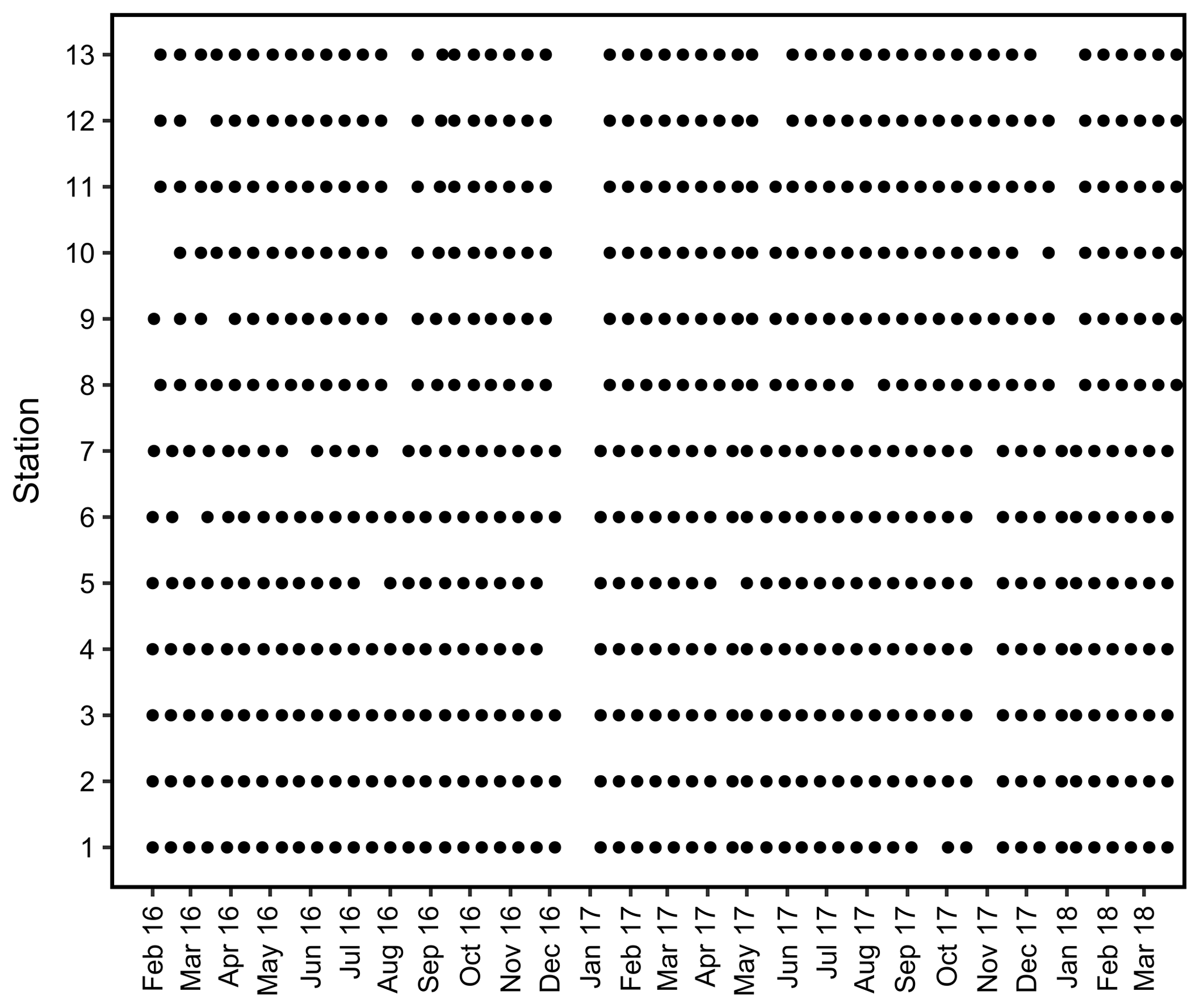
Figure 3Data availability of dissolved inorganic nutrient concentrations. Each dot represents a measurement for total oxidized nitrogen, nitrite, ammonia, phosphate and silicate.
3.2 Temperature, salinity and dissolved oxygen
Records of temperature, salinity and DO concentration are available from 16 February 2016 to 23 May 2018 (Fig. 4). Missing data resulted from readouts and sensor malfunctions (Table 3). For Station 6 no data from the logger station are available due to complete failure of the deployed data loggers. Datasets of Stations 3, 5, 8 and 11 end in 2017, as the logger stations were not found back at the last readout date (Table 3), probably due to sedimentation processes. On average, 96 % of records for temperature, salinity and DO concentration were retained from the raw dataset after data processing (see Sect. 2.4.2) and a mean data availability of 671 d (1.8 years) was reached. On average, more data are available for salinity and temperature (690 d) than for DO content (653 d). For each station and logger type a single data file is given at PANGAEA.
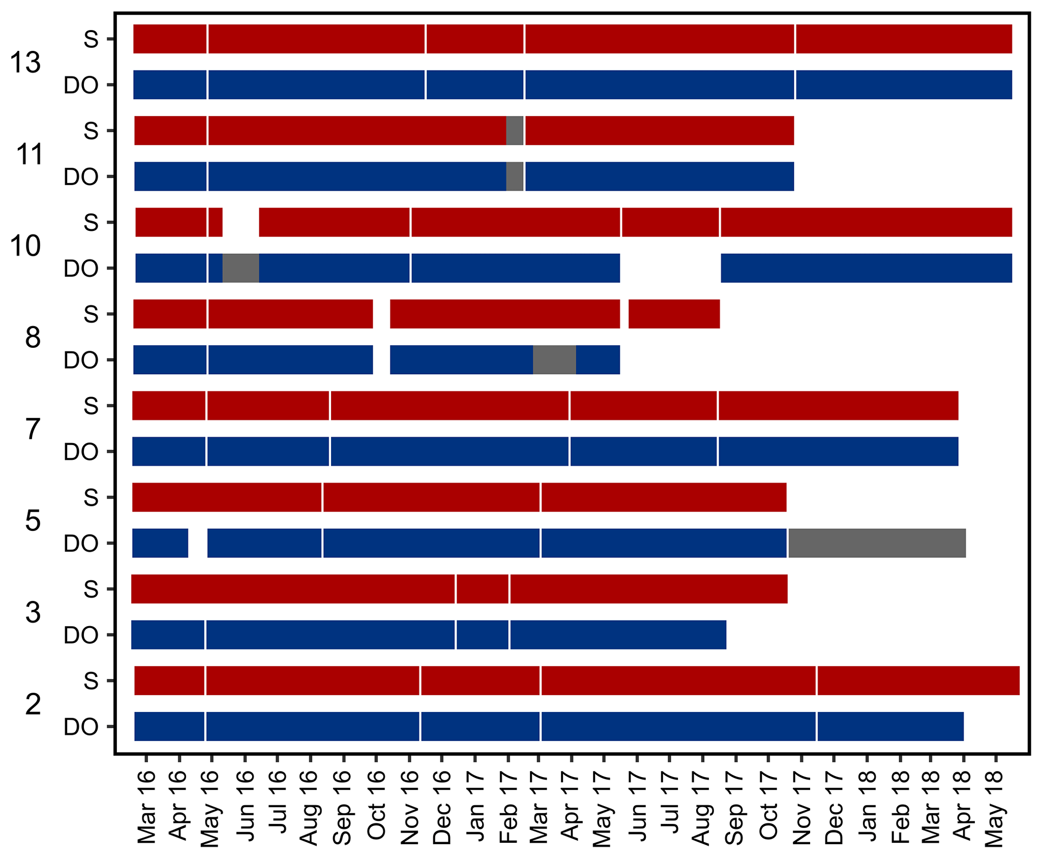
Figure 4Data availability of dissolved oxygen (DO) concentration and salinity measured by self-contained data loggers. Both logger types (DO and salinity) additionally measured temperature. Temperature data are always available for the same periods as DO and salinity. Grey bars indicate cases where only temperature data are available. Y axis shows station numbers and respective logger type. Note that only data with a quality flag of 1 are considered.
4.1 Dissolved inorganic nutrients
The measurements of nitrate concentrations exhibited differences between monitoring stations. Interquartile ranges (IQRs) were higher for Stations 11–13 than for the remaining ones (Fig. 5a). All stations showed numerous outliers (values >1.5 times IQR), with the highest values measured for Station 13. Overall nitrate concentrations range between 0 and 121.41 µmol L−1 (Table 5).

Figure 5Box plots of measured dissolved inorganic nutrient concentrations. Data for nitrate (a), nitrite (b), ammonia (c), phosphate (d) and silicate (e) concentrations are presented. X axis indicates station numbers. Boxes indicate the median and first and third quartiles. Whiskers show values within and dots values outside 1.5 times the interquartile range.
Table 5Summary of measured dissolved inorganic nutrient concentrations in water samples from the monitoring stations. For each station and nutrient, median, minimum and maximum concentrations are presented.

The records for nitrite concentrations show larger IQRs in general. Here, Stations 1 and 4 as well as 11–13 are found to be more variable than the other stations (Fig. 5b). The outliers are evenly distributed over all stations. Nitrite concentrations range between 0 and 1.04 µmol L−1, with the highest measurements recorded for Station 13 (Table 5).
The measured concentrations for ammonia show a similar variability as the records for nitrate concentrations. The highest IQRs are again found for Stations 11–13. Moreover, Station 13 exhibited the highest ammonia concentrations measured (Fig. 5c). Concentrations of ammonia range between 0.43 and 17.46 µmol L−1 (Table 5).
The phosphate concentrations show low variability over all stations (Fig. 5d). Among all dissolved inorganic nutrients measured, phosphate reveals the lowest number of outliers, with Stations 4, 7, 8, 10 and 11 being without outliers at all. The highest concentration of phosphate was recorded for Station 3. In total, concentrations range between 0.04 and 3.39 µmol L−1 (Table 5).
The measured silicate concentrations display comparable variabilities like the measurements for phosphate concentrations. Stations 1 and 4 as well as 11–13 feature slightly larger IQRs than the other stations (Fig. 5e). Noticeably, Stations 7–9 exhibit no outliers. At Station 13, the highest concentration of silicate was registered. The data for silicate concentrations range between 0 and 67.66 µmol L−1 (Table 5).
4.2 Temperature, salinity and dissolved oxygen
Temperature data show little variation between the different monitoring stations, indicated by largely overlapping box plots (Fig. 6a, c). The records range between 0 and 22 ∘C (Table 6), with a maximum daily change in temperature of 8 ∘C in May 2017 (Station 13). As a result of a shorter monitoring period (Fig. 4), medians of Stations 3, 5 and 11 tend to be higher than the remaining ones. The records of temperature at these stations end in October 2017 and therefore the medians were not influenced by low temperatures in winter 2017 and spring 2018.

Figure 6Box plots of temperature, salinity and dissolved oxygen concentration recorded over the monitoring period by DST CT (a, b) and MiniDOT (c, d) data loggers, respectively. X axis indicates station numbers. Boxes indicate median, first and third quartile. Whiskers show values within and dots values outside 1.5-times interquartile range. Note that only data with quality flag =1 were plotted.
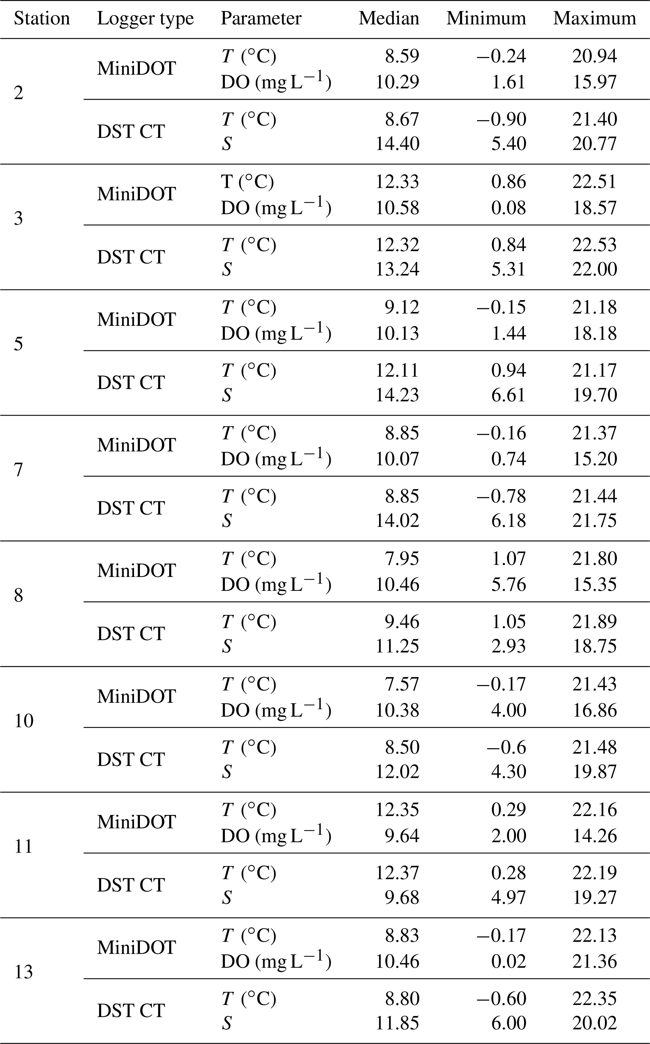
Table 6Median and range of recorded measurements obtained by self-contained data loggers over the respective monitoring period. Temperature (T), dissolved oxygen concentration (DO) and salinity (S) were measured by two types of data loggers. Note that data can cover different time periods (see Sect. 3.2) and that only data with a quality flag of 1 were considered.
Data indicate a decrease in salinity of 0.02 per kilometer (regression: , p=0.013) from Station 2 to Station 13 (Fig. 6b). This represents an overall decrease in salinity of 3.8 over a straight-line distance of 174 km. Variability among the stations is very similar, overall values range between salinities of 3 and 22 (Table 6). The largest fluctuation in salinity within a single day was recorded in March 2017 at Station 13 with a change of 9. The highest measurements were recorded for Stations 3 and 7, the lowest for Station 8.
Measurements of DO concentration showed consistently similar medians for all stations (Fig. 6d). Noticeably, the variability among the stations differed. Data of Station 8 range between 6 and 15 mg L−1, while data of Station 13 vary between 0 and 21 mg L−1 (Table 6). For the latter, the largest daily range of 15 mg L−1 was recorded in August 2016.
The exemplary detailed comparison of Stations 2 and 13 reveals substantial differences in variability and seasonal dynamics of the measured variables (Fig. 7). Temperature, being the least fluctuating measurement, shows no apparent differences in its overall trends (Fig. 7a). However, the variability in summer months tends to be more pronounced at Station 13, especially visible in summer 2017. The salinity records for both stations do not follow a seasonal pattern, e.g., showing steep increases in summer 2016 as well as winter 2017 (Station 2, Fig. 7b). Noticeably, shorter-term fluctuations (within a month) appear to be more common at Station 13, being especially strong in spring to summer 2017. The data for DO concentration show great differences in the degree of short-term variability among the two compared stations (Fig. 7c). Here, Station 2 is again less variable, displaying a more compressed trend. In contrast, DO concentrations at Station 13 vary strongly within short time frames (a few days) with differences of up to ∼15 mg L−1 , e.g., in summer 2017 (Fig. 7c). In addition to spatial differences in variability, fluctuations of DO concentrations are generally amplified in spring to autumn at both stations.
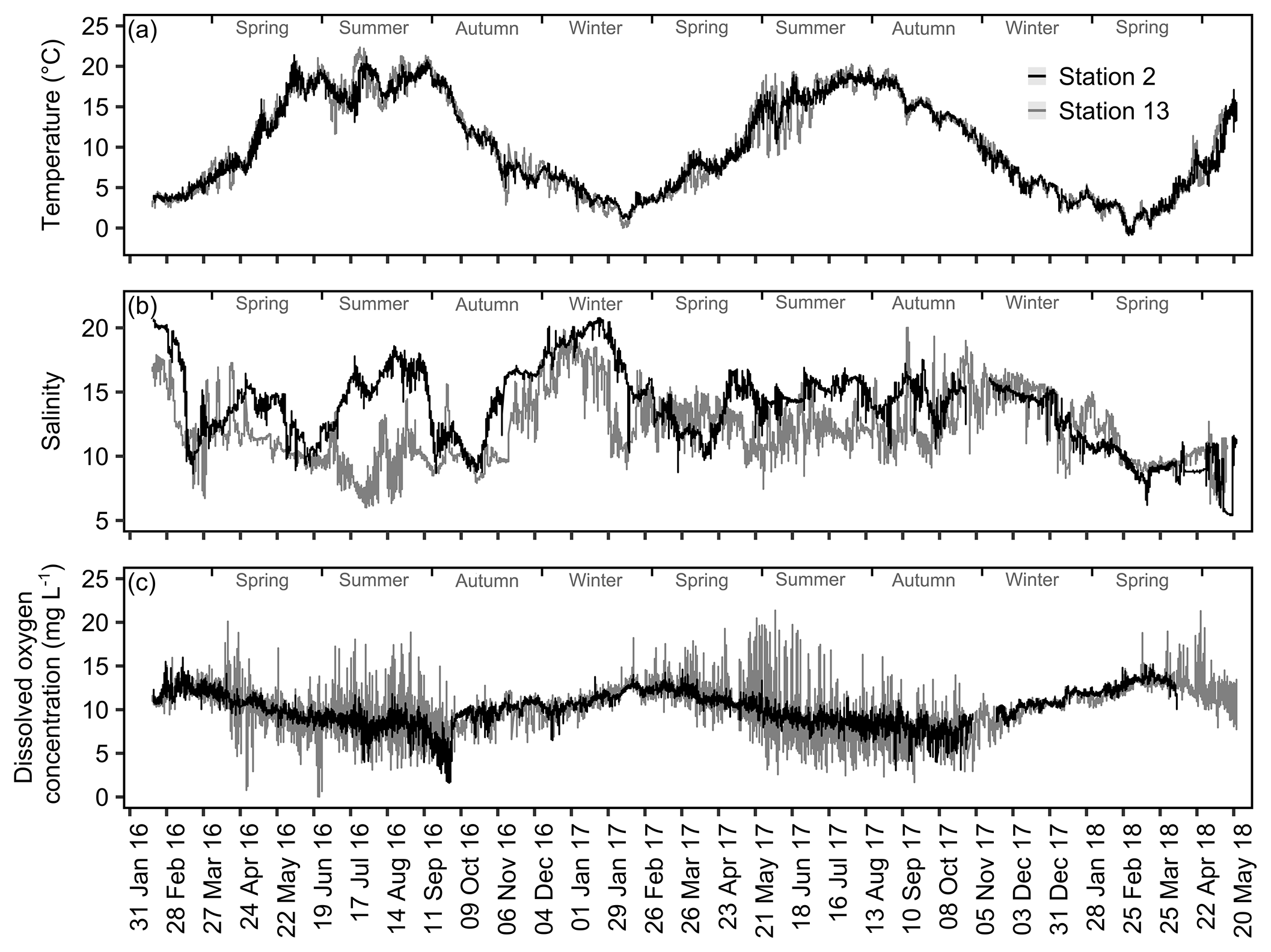
Figure 7Exemplary overview of temperature (a), salinity (b) and dissolved oxygen concentration (c) datasets for Stations 2 and 13. The presented data were recorded by DST CT (a, b) and MiniDOT (c) data loggers. Note that only data with a quality flag of 1 were plotted.
The present environmental monitoring provides data for dissolved inorganic nutrient contents recorded twice a month and continuous records of temperature, salinity and DO concentration. The obtained data provide a good picture of the highly dynamic shallow waters at the Baltic coast of Schleswig-Holstein, Germany. The total range (Fig. 6) as well as the recorded maximum diurnal changes (see Sect. 4.2) of continuously measured parameters highlight the enormous environmental fluctuations biota are facing in these habitats. However, the closer examination of data obtained for Stations 2 and 13, which were exemplarily depicted, shows that the extent of environmental variability locally depends on spatial and temporal factors (Fig. 7). This is especially evident for measurements of salinity and DO concentration. At both stations, the trends in salinity neither followed a recurring seasonal pattern nor was there a systematic difference between the stations, which could be expected according to the results of the applied regression using median salinities of the overall monitoring period (see Sect. 4.2). In contrast, the observed fluctuations have different timings at the stations, indicating that local influences like rainwater discharges could co-occur with large-scale processes, e.g., inflow events of North Atlantic waters (Snoeijs-Leijonmalm et al., 2017; Reusch et al., 2018). Local factors might also explain the rapid increase in salinity within a single day at Station 13 that was paralleled by DO concentrations dropping to 1.7 mg L−1, an indication of oxygen-depleted water being upwelled at the coast. The variability of measured DO concentrations also exhibits local differences and, in addition, seasonal patterns. The overall stronger variability of DO data at Station 13 could be related to higher nutrient loads compared to Station 2. The median nitrate concentrations at this station were 2 times higher; the recorded maximum exceeded even 7.5 times the value of Station 2 (Table 5). In consequence, biological productivity could be enhanced at this station, leading to larger diurnal fluctuations (Gubelit and Berezina, 2010), e.g., recorded as a drop by 50 % in DO concentration in August 2016. The generally lower variability in winter at both stations could be mediated by lower temperatures since biological processes are slowed down in this period, keeping oxygen concentrations more stable. The likelihood of detecting such events and processes by repeated single measurements is very low; thus continuous records provide the chance to unravel short-term dynamics that might have not been described by common monitoring efforts.
The measured nutrient loads exhibited seasonal fluctuations with the highest concentrations in autumn and winter (Fig. 5). Noticeably, the present extremes in nitrate concentrations exceed 6.6 times the highest recorded concentration measured at a close-by time series station between 1957 and 2014 at a depth of 1 m (https://www.bokniseck.de/, last access: 1 July 2019; Lennartz et al., 2014; Bange and Malien, 2015). The Boknis Eck time series station is situated 2.2 km away from Station 3, but located further offshore. Therefore, the time series station could be less affected by local river runoff and groundwater seepage that might explain the increased nitrate loads in water samples of this study (Szymczycha and Pempkowiak, 2016). Indeed, groundwater seepage has been described as a significant pathway in the hydrology of Eckernförde Bay (Schlüter et al., 2004), a location that is covered in this monitoring and where measured nitrate concentrations were among the highest (Stations 3 and 4; see Table 5).
The employment of self-contained monitoring systems, as presented here, always poses the risk of data losses due to failure of data loggers. Since the used data loggers have to be read out manually, a malfunction could be detected with temporal delay, leading to substantial gaps in the records. Real-time data systems like measurement buoys provide the advantage of wireless data transmission, allowing a continuous control of functionality. Furthermore, sensors attached to buoys are less susceptible to sediment dynamics. The coverage of the logger station by sand will potentially lead to extended gaps in coming datasets since four of the setups were not found during the last readout. Nevertheless, the advantages of real-time data systems go along with an increase in expenses for single measurement systems by up to an order of magnitude. Therefore, in this study, independent data loggers have been applied, keeping costs lower and favoring a higher replication of the measurement stations. The average retained number of data (96 %) from the raw dataset of temperature, salinity and DO measurements shows that this strategy can be a worthwhile alternative to more expensive monitoring systems. For future deployments the geological characteristics of the sampling sites should be examined in more detail, e.g., to avoid areas of pronounced sediment transport.
The obtained, temporally fine-scaled data of this study could be utilized for diverse purposes. The records could support the development and skill assessment of models (oceanographic, biogeochemical and ecological) or provide background information for the definition and probability of extreme events like heat waves or coastal upwelling (Bennett et al., 2013; Hobday et al., 2016; Bates et al., 2018). It may serve as a base for more realistic experimental approaches that not only apply mean treatment levels but also consider the range and magnitude of environmental variation (Wernberg et al., 2012). Moreover, the data could help to identify mechanisms behind observed changes in biological monitoring programs performed in the same area. Since the assessment will be continued for the coming years, the temporal coverage of the dataset is going to broaden in the future and may even enhance its applicability.
Versatile possible uses of the presented data underline the great value of observational programs. As the human population is concentrated along the coastlines, signals of anthropogenic changes are expected to be particularly strong. However, the detection of change in coastal areas is a challenging task since human pressures and natural variability caused by the sea–land interface vastly overlap (Cloern et al., 2016). At this point, environmental data of high resolution can be a useful tool, as they allow a better differentiation of natural variability from signs of human impact. Traditional monitoring strategies (e.g., ship-based surveys) can usually not provide the necessary information since temporal resolution is low and access to shallow waters limited. Self-contained monitoring systems therefore appear as a suitable alternative to bridge this knowledge gap. The presented approach displays an opportunity not only to researchers in better understanding the system dynamics, but also for policymakers in choosing appropriate measures in future environmental protection (Helmuth et al., 2014).
MF wrote the paper and processed the raw data. CL and GB performed maintenance of the logger stations as well as samplings for nutrient analyses. RK initiated and designed the monitoring program. All authors participated in data logger readouts.
The authors declare that they have no conflict of interest.
We would like to thank Vanessa Herhoffer for her conscientious work collecting water samples, Bente Gardeler for nutrient analyses, and various divers for help in finding and maintaining logger stations.
This research is supported by the “State Agency for Agriculture, Environment and Rural Areas of Schleswig-Holstein” (LLUR; reference number: 0608.451426).
This paper was edited by Giuseppe M. R. Manzella and reviewed by two anonymous referees.
Babulak, S. W. and Gildenberg, L.: Automated determination of silicate and carbonates in detergents, J. Am. Oil Chem. Soc., 50, 296–299, 1973.
Bange, H. W. and Malien, F.: Hydrochemistry from time series station Boknis Eck from 1957 to 2014, PANGAEA, https://doi.org/10.1594/PANGAEA.855693, 2015.
Bates, A. E., Helmuth, B., Burrows, M. T., Duncan, M. I., Garrabou, J., Guy-Haim, T., Lima, F., Queiros, A. M., Seabra, R., Marsh, R., Belmaker, J., Bensoussan, N., Dong, Y., Mazaris, A. D., Smale, D., Wahl, M., and Rilov, G.: Biologists ignore ocean weather at their peril, Nature, 560, 299–301, https://doi.org/10.1038/d41586-018-05869-5, 2018.
Bennett, N. D., Croke, B. F. W., Guariso, G., Guillaume, J. H. A., Hamilton, S. H., Jakeman, A. J., Marsili-Libelli, S., Newham, L. T. H., Norton, J. P., Perrin, C., Pierce, S. A., Robson, B., Seppelt, R., Voinov, A. A., Fath, B. D., and Andreassian, V.: Characterising performance of environmental models, Environ. Model. Softw., 40, 1–20, https://doi.org/10.1016/j.envsoft.2012.09.011, 2013.
Benson, B. B. and Krause Jr, D.: The concentration and isotopic fractionation of oxygen dissolved in freshwater and seawater in equilibrium with the atmosphere, Limnol. Oceanogr., 29, 620–632, https://doi.org/10.1016/0198-0254(84)93289-8, 1984.
Boltz, D. F. and Mellon, M. G.: Spectrophotometric determination of phosphorus as molybdiphosphoric acid, Anal. Chem., 20, 749–751, 1948.
Carstensen, J., Andersen, J. H., Gustafsson, B. G., and Conley, D. J.: Deoxygenation of the Baltic Sea during the last century, P. Natl. Acad. Sci. USA, 111, 5628–5633, https://doi.org/10.1073/pnas.1323156111, 2014.
Cloern, J. E., Abreu, P. C., Carstensen, J., Chauvaud, L., Elmgren, R., Grall, J., Greening, H., Johansson, J. O. R., Kahru, M., Sherwood, E. T., Xu, J., and Yin, K.: Human activities and climate variability drive fast-paced change across the world's estuarine-coastal ecosystems, Glob. Change Biol., 22, 513–529, https://doi.org/10.1111/gcb.13059, 2016.
Conley, D. J., Carstensen, J., Aigars, J., Axe, P., Bonsdorff, E., Eremina, T., Haahti, B.-M., Humborg, C., Jonsson, P., Kotta, J., Lännegren, C., Larsson, U., Maximov, A., Rodriguez Medina, M., Lysiak-Pastuszak, E., Remeikaitė-Nikienė, N., Walve, J., Wilhelms, S., and Zillén, L.: Hypoxia Is Increasing in the Coastal Zone of the Baltic Sea, Environ. Sci. Technol., 45, 6777–6783, https://doi.org/10.1021/es201212r, 2011.
EPA: Method of chemical analysis of water and wastes, Off Technological Transfer, Environmental Protection Agency, Washington D.C., 1974.
Franz, M., Lieberum, C., Bock, G., and Karez, R.: Environmental parameters of shallow water habitats in the SW Baltic Sea, GEOMAR Helmholtz Centre for Ocean Research Kiel, Germany, PANGAEA, https://doi.org/10.1594/PANGAEA.895257, 2018.
Garcia, H. E. and Gordon, L. I.: Oxygen solubility in seawater: Better fitting equations, Limnol. Oceanogr., 37, 1307–1312, https://doi.org/10.4319/lo.1992.37.6.1307, 1992.
Garel, E. and Ferreira, Ó.: Multi-year high-frequency physical and environmental observations at the Guadiana Estuary, Earth Syst. Sci. Data, 7, 299–309, https://doi.org/10.5194/essd-7-299-2015, 2015.
Greenberg, A. E., Jenkins, D., and Connors, J. J.: Standard methods for the examination of water and wastewater, 15th edn., APHA-AWWA-WPCF, 1980.
Gubelit, Y. I. and Berezina, N. A.: The causes and consequences of algal blooms: The Cladophora glomerata bloom and the Neva estuary (eastern Baltic Sea), Mar. Pollut. Bull., 61, 183–188, https://doi.org/10.1016/j.marpolbul.2010.02.013, 2010.
HELCOM: Thematic assessment of eutrophication 2011–2016, available at: http://www.helcom.fi/baltic-sea-trends/holistic-assessments/state-of-the-baltic-sea-2018/reports-and-materials/ (last access: 1 July 2019), 2018.
Helmuth, B., Russell, B. D., Connell, S. D., Dong, Y., Harley, C. D., Lima, F. P., Sará, G., Williams, G. A., and Mieszkowska, N.: Beyond long-term averages: making biological sense of a rapidly changing world, Climate Change Responses, 1, 1–12, https://doi.org/10.1186/s40665-014-0006-0, 2014.
Hobday, A. J., Alexander, L. V, Perkins, S. E., Smale, D. A., Straub, S. C., Oliver, E. C. J., Benthuysen, J. A., Burrows, M. T., Donat, M. G., Feng, M., Holbrook, N. J., Moore, P. J., Scannell, H. A., Sen Gupta, A. and Wernberg, T.: A hierarchical approach to defining marine heatwaves, Prog. Oceanogr., 141, 227–238, https://doi.org/10.1016/j.pocean.2015.12.014, 2016.
ISO 3696: Water for analytical laboratory use – Specification and test methods, 1987.
ISO 13395: Water quality – Determination of nitrite nitrogen and nitrate nitrogen and the sum of both by flow analysis (CFA and FIA) and spectrometric detection, 1996.
ISO 16264: Water quality – Determination of soluble silicates by flow analysis (FIA and CFA) and photometric detection, 2002.
ISO 15681-2: Water quality – Determination of orthophosphate and total phosphorus contents by flow analysis (FIA and CFA) – Part 2: Method by continuous flow analysis (CFA), 2003.
Jonsson, P. R., Kotta, J., Andersson, H. C., Herkül, K., Virtanen, E., Sandman, A. N., and Johannesson, K.: High climate velocity and population fragmentation may constrain climate-driven range shift of the key habitat former Fucus vesiculosus, Divers. Distrib., 24, 892–905, https://doi.org/10.1111/ddi.12733, 2018.
Krom, M. D.: Spectrophotometric determination of ammonia: a study of a modified Berthelot reaction using salicylate and dichloroisocyanurate, Analyst, 105, 305–316, 1980.
Lehmann, A. and Myrberg, K.: Upwelling in the Baltic Sea – A review, J. Marine Syst., 74, 3–12, https://doi.org/10.1016/j.jmarsys.2008.02.010, 2008.
Lennartz, S. T., Lehmann, A., Herrford, J., Malien, F., Hansen, H.-P., Biester, H., and Bange, H. W.: Long-term trends at the Boknis Eck time series station (Baltic Sea), 1957–2013: does climate change counteract the decline in eutrophication?, Biogeosciences, 11, 6323–6339, https://doi.org/10.5194/bg-11-6323-2014, 2014.
Mills, K., Pershing, A., Brown, C., Chen, Y., Chiang, F.-S., Holland, D., Lehuta, S., Nye, J., Sun, J., Thomas, A., and Wahle, R.: Fisheries management in a changing climate: Lessons from the 2012 ocean heat wave in the Northwest Atlantic, Oceanography, 26, 191–195, https://doi.org/10.5670/oceanog.2013.27, 2013.
Navone, R.: Proposed method for nitrate in potable waters, J. Am. Water Works Ass., 56, 781–783, 1964.
Reusch, T. B. H., Dierking, J., Andersson, H. C., Bonsdorff, E., Carstensen, J., Casini, M., Czajkowski, M., Hasler, B., Hinsby, K., Hyytiäinen, K., Johannesson, K., Jomaa, S., Jormalainen, V., Kuosa, H., Kurland, S., Laikre, L., MacKenzie, B. R., Margonski, P., Melzner, F., Oesterwind, D., Ojaveer, H., Refsgaard, J. C., Sandström, A., Schwarz, G., Tonderski, K., Winder, M., and Zandersen, M.: The Baltic Sea as a time machine for the future coastal ocean, Science Advances, 4, eaar8195, https://doi.org/10.1126/sciadv.aar8195, 2018.
Saderne, V., Fietzek, P., and Herman, P. M. J.: Extreme Variations of pCO2 and pH in a Macrophyte Meadow of the Baltic Sea in Summer: Evidence of the Effect of Photosynthesis and Local Upwelling, PLoS One, 8, e62689, https://doi.org/10.1371/journal.pone.0062689, 2013.
Schlüter, M., Sauter, E. J., Andersen, C. E., Dahlgaard, H., and Dando, P. R.: Spatial distribution and budget for submarine groundwater discharge in Eckernförde Bay (Western Baltic Sea), Limnol. Oceanogr., 49, 157–167, https://doi.org/10.4319/lo.2004.49.1.0157, 2004.
Searle, P. L.: The Berthelot or indophenol reaction and its use in the analytical chemistry of nitrogen, A review, Analyst, 109, 549–568, 1984.
Sinex, C. H.: Coping with variability in the coastal environment, Proceedings of OCEANS'94, Brest, France, 13–16 September 1994, IEEE, 2, II/1–II/6, https://doi.org/10.1109/OCEANS.1994.364005, 1994.
Smith, J. D. and Milne, P. J.: Spectrophotometric determination of silicate in natural waters by formation of α-molybdosilicic acid and reduction with a tin (IV)-ascorbic acid-oxalic acid mixture, Anal. Chim. Acta, 123, 263–270, 1981.
Snoeijs-Leijonmalm, P., Schubert, H., and Radziejewska, T. (Eds.): Biological Oceanography of the Baltic Sea, Springer Netherlands, Dordrecht, https://doi.org/10.1007/978-94-007-0668-2, 2017.
Szymczycha, B. and Pempkowiak, J.: The Role of Submarine Groundwater Discharge as Material Source to the Baltic Sea, Springer International Publishing, Switzerland, https://doi.org/10.1007/978-3-319-25960-4, 2016.
Walinga, I., Van Vark, W., Houba, V. J. G., and der Lee, J. J.: Soil and plant analysis, Part 7, Plant Anal. Proced. Syllabus, Wageningen Agricultural University, Wageningen, Neatherlands, 1989.
Wernberg, T., Smale, D. A., and Thomsen M. S.: A decade of climate change experiments on marine organisms: procedures, patterns and problems, Glob. Change Biol., 18, 1491–1498, https://doi.org/10.1111/j.1365-2486.2012.02656.x, 2012.