the Creative Commons Attribution 4.0 License.
the Creative Commons Attribution 4.0 License.
 | 08 Jul 2019
EDGAR v4.3.2 Global Atlas of the three major greenhouse gas emissions for the period 1970–2012
Greet Janssens-Maenhout
Monica Crippa
Diego Guizzardi
Marilena Muntean
Edwin Schaaf
Frank Dentener
Peter Bergamaschi
Valerio Pagliari
Jos G. J. Olivier
Jeroen A. H. W. Peters
John A. van Aardenne
Suvi Monni
Ulrike Doering
A. M. Roxana Petrescu
Efisio Solazzo
Gabriel D. Oreggioni
The Emissions Database for Global Atmospheric Research (EDGAR) compiles anthropogenic emissions data for greenhouse gases (GHGs), and for multiple air pollutants, based on international statistics and emission factors. EDGAR data provide quantitative support for atmospheric modelling and for mitigation scenario and impact assessment analyses as well as for policy evaluation. The new version (v4.3.2) of the EDGAR emission inventory provides global estimates, broken down to IPCC-relevant source-sector levels, from 1970 (the year of the European Union's first Air Quality Directive) to 2012 (the end year of the first commitment period of the Kyoto Protocol, KP). Strengths of EDGAR v4.3.2 include global geo-coverage (226 countries), continuity in time, and comprehensiveness in activities. Emissions of multiple chemical compounds, GHGs as well as air pollutants, from relevant sources (fossil fuel activities but also, for example, fermentation processes in agricultural activities) are compiled following a bottom-up (BU), transparent and IPCC-compliant methodology. This paper describes EDGAR v4.3.2 developments with respect to three major long-lived GHGs (CO2, CH4, and N2O) derived from a wide range of human activities apart from the land-use, land-use change and forestry (LULUCF) sector and apart from savannah burning; a companion paper quantifies and discusses emissions of air pollutants. Detailed information is included for each of the IPCC-relevant source sectors, leading to global totals for 2010 (in the middle of the first KP commitment period) (with a 95 % confidence interval in parentheses): 33.6(±5.9) Pg CO2 yr−1, 0.34(±0.16) Pg CH4 yr−1, and 7.2(±3.7) Tg N2O yr−1. We provide uncertainty factors in emissions data for the different GHGs and for three different groups of countries: OECD countries of 1990, countries with economies in transition in 1990, and the remaining countries in development (the UNFCCC non-Annex I parties). We document trends for the major emitting countries together with the European Union in more detail, demonstrating that effects of fuel markets and financial instability have had greater impacts on GHG trends than effects of income or population. These data (https://doi.org/10.5281/zenodo.2658138, Janssens-Maenhout et al., 2019) are visualised with annual and monthly global emissions grid maps of for each source sector.
- Article
(14981 KB) -
Supplement
(1741 KB) - BibTeX
- EndNote


An essential component of the UN Framework Convention on Climate Change (UNFCCC, 1992) is the collection of nationally reported inventories and information on these greenhouse gas (GHG) emission inventory time series. At the time the UNFCCC was established, the 24 members of the OECD in 1990 and 16 other European countries and Russia were considered liable for “the largest share of historical and current global emissions of GHG” and taken up in Annex I to the UNFCCC. These Annex I countries and the European Union1 submit annually complete inventories of GHG emissions from the 1990 base year2 until the latest year for which full accounting is completed and reviewed (typically with a 2-year time lag), and these inventories are all reviewed to ensure transparency, completeness, comparability, consistency and accuracy3. This allows for most of these Annex I countries to track progress towards their reduction targets committed under the Kyoto Protocol (UNFCCC, 1997). Other (non-Annex I) countries are encouraged to submit their GHG inventories as part of their National Communications and Biennial Update Reports (BURs). The GHG inventories of non-Annex I countries were required to cover CO2, CH4 and N2O emissions for 1 year (1990 or 1994), without specific documentation and only subject to a brief review. However, the Paris Agreement (UNFCCC, 2015) requires submission every 2 years of BURs4, which are subject to international consultation and analysis. Theoretically, UNFCCC should receive at the latest after 2 years national emissions inventories from each of the 197 countries, but as shown in Fig. 1a, not all countries did provide a national inventory and 154 countries did not provide a completed (i.e. year-2) time series of inventories. In addition, many countries lack a well-developed statistical infrastructure, which is needed for an accurate bottom-up (BU) inventory. Figure 1b presents the latest year that is covered with a national inventory, with dates for quite a few countries more than 10 years ago: for most South-East Asian countries this is between 2004 and 2007 and for most African countries between 2000 and 2003.

Figure 1(a) Inventory submission as received at UNFCCC (by January 2017) for all countries: expressed with the year of emission reporting in which the latest national communication to UNFCCC took place. (b) Inventory submission as received at UNFCCC (by January 2017) for all countries expressed with the latest year of emission that is covered in the inventory submitted to UNFCCC.
As such, the collection of national reports/communications does not provide a complete, consistent and comparable global dataset which can be used to understand the global budgets of the most important GHG emissions and their impact on climate. Very few bottom-up inventories of global anthropogenic emissions have been produced with continued effort for more than 2 decades. The Carbon Dioxide Information Analysis Centre (CDIAC) (Boden et al., 2017; Andres et al., 2014) and the Emissions Database for Global Atmospheric Research (EDGAR) (Olivier and Janssens-Maenhout, 2016; Olivier et al., 2016) provide global totals, whereas the IEA provides CO2 estimates from fuel combustion only and the FAO CH4 from agriculture only. While CDIAC ceased operation in September 2017, the Open-source Data Inventory for Anthropogenic CO2 (ODIAC) (Oda et al., 2018) continued to use the CDIAC data and combined these with geospatial proxies (including night light satellite maps) to provide CO2 grid maps, as EDGAR is also doing (using other geospatial proxies). In addition, the new Community Emissions Data System (CEDS) of Hoesly et al. (2018) builds upon existing inventories to provide a new gridded dataset of all emission species for the Climate Model Inter-comparison Programme CMIP6.
The scientific community started to bring together these anthropogenic BU emissions with top-down estimates covering also the natural component to obtain the Global Carbon Budget (GCB) (Le Quéré et al., 2018) and the Global Methane Budget (Saunois et al., 2016). These budgets are important input for the periodic global stocktake that the Paris Agreement envisages from 2023 onwards (with the submitted inventories for 2021). Even though significant progress in inventory compilation has been made, the overall uncertainty of the global total has become larger over time because the share of emissions from non-Annex I countries (with less developed statistical infrastructure) increased from less than 40 % in 1990 to more than 60 % in 2012, as shown in Fig. 2.

Figure 2Relative contribution of the Annex I and non-Annex I countries to the global total GHG emissions. The red, brown and orange dashed parts of the stack correspond to the non-Annex I share that increases from about 1∕3 in 1990 to almost 2∕3 in 2012.
To support both science and policy making with the monitoring and verification of the GHG emissions, it is important that emissions are estimated by using comparable methodologies, consistent source allocation and comprehensive coverage of the globe. The EDGAR v4.3.2 global inventory illustrates the result of a bottom-up technology-based compilation of country- and sector-specific emission time series for 1970–2012. Furthermore, the monthly resolution and global grid maps at a spatial resolution of allow direct use in atmospheric models as well as in analyses of policy impacts. The first version of the Emissions Database for Global Atmospheric Research (EDGAR v2) answered the needs of the air quality community to map technological parameters of air pollution sources and was published by Olivier et al. (1996). Since then, several updated versions (Olivier, 2002) have been released (EDGAR-HYDE, EDGAR v3.2, EDGAR 3.2 FT2000). Driven by the development of scientific knowledge on emission generating processes and by the availability of more recent information, the EDGAR v4 datasets were constructed including new emission factors and additional end-of-pipe abatement measures. The specification of the combustion technology and its end-of-pipe abatement is more important for air pollutants and aerosols than for GHGs. CO2 combustion emissions are fuel-determined and carbon capture and storage are not yet implemented at an operational level and are not considered here. However, abatement is considered for e.g. CH4 recovery of coal mines, and technology and end-of-pipe abatement are important for both adipic and nitric acid plants. Finally, management of crop cultivation (e.g. for rice) or of manure are accounted for by technology-specific emission factors for CH4 and N2O.
Previous EDGAR versions v4.1 and v4.2 (available at http://edgar.jrc.ec.europa.eu/index.php#) are interim frozen datasets without peer-reviewed documentation, but are nevertheless extensively used by modellers. Illustrative examples of the EDGAR v4 use are given in Table S5 in the Supplement. The new online version of EDGAR v4.3.2 is the main reference for the EDGAR v4 datasets, and is the subject of this paper. We wish to stress that EDGAR v4.3.2 is the result of a steady improvement of the EDGAR v4 database over more than a decade, also thanks to the feedback of users. For the main differences between EDGAR v4.3.2 and v 4.2, we refer the reader to the Supplement of the paper, Sect. 3 and Table S5 with the findings of atmospheric studies using EDGAR v4 as input. For the main differences between EDGAR v4.2 and v4.1, we refer the reader to http://edgar.jrc.ec.europa.eu/Main_differences_between_EDGARv42_and_v41.pdf.
In this paper we focus on the three key GHG emission components of EDGAR v4.3.2, describing the methodology, emission sources, activity data, emission factors and emission disaggregation (in space and time). For CO2 we distinguish between (i) long-cycle carbon CO2 from fossil fuel use and industrial processes (cement production, carbonate use of limestone and dolomite, non-energy use of fuels and other combustion, chemical and metal processes, solvents, agricultural liming and urea, waste and fossil fuel fires) and (ii) short-cycle carbon CO2 from biofuel use or short-cycle biomass burning (such as agricultural waste burning). The non-CO2 GHG emissions are also provided to the IEA for the annual publication of emissions from fuel combustion (Olivier and Janssens-Maenhout, 2016). The EDGAR v4.3.2 frozen dataset for 1970–2012 is used to produce the updates from 2013 onwards, derived with a fast track (FT) approach (e.g. EDGAR v4.3.2_FT2016). Under the FT update the activities are grouped into five main source sectors and for each of the latter trends of the most recent activity statistics are used. These are derived from data provided by the latest IEA (2016) and BP (2017) statistics in terms of fuel trend indicators that are applied to the fossil fuel combustion sector. For the other main sectors we use most recent commodity statistics from the US Geological Survey, the World Steel Association and the International Fertiliser Association, as explained in more detail in Olivier et al. (2016). The methodology and activity data are also used to estimate corresponding gaseous and particulate air pollutant emissions, as part II of the EDGAR v4.3.2 release (Crippa et al., 2018). Other EDGAR v4 air pollutants inventories are EDGAR v4.3.1 (Crippa et al., 2016a; Huang et al., 2017), EDGAR v4tox1 (Muntean et al., 2014) and EDGAR v4tox2 (Muntean et al., 2018).
2.1 Bottom-up emission calculation
Annual country-specific emissions are calculated using international activity data and emission factors, updated according to the latest scientific knowledge and following IPCC (2006a) methods. Emissions (EMs) from a given sector i in a country C accumulated during a year t for a chemical compound x are calculated with the country-specific activity data (AD), quantifying the activity for sector i, with the mix of j technologies (TECH) and with the mix of k (end-of-pipe) abatement measures (EOP) installed with share k for each technology j, the emission rate with an uncontrolled emission factor (EF) for each sector i and technology j and relative reduction (RED) by abatement measure k, as summarised in the following formula:
The activity data are very sector dependent and vary from fuel consumption in energy units (TJ) of a particular fuel type, to the amount (ton) of products manufactured, and to the number of animals or the area (hectares) and yield (ton) of cultivated crops. The technology mixes, (uncontrolled5) emission factors and end-of-pipe measures are determined at different levels: country-specific, regional, country group (e.g. Annex I/non-Annex I), or global. Technology-specific emission factors are used to allow a tier-2 approach, taking into account the different management/technology processes or infrastructures (e.g. different distribution networks) under specific “technologies”, and modelling explicitly abatements/reductions, e.g. the CH4 recovery from coal mine gas at country level under the “end-of-pipe measures”. Just as with national inventories, EDGAR v4.3.2 starts from accounting over a period of time, 1 calendar year, and over a well-defined region, the country in which the emissions took place.
The sector-specific total emissions of substance x for country C in year t are then distributed in time and space using sector- and even technology-specific monthly shares m and spatial proxy datasets f. The proxy datasets are expressed as a function of coordinates (longitude, latitude) weighted at country level and with the Heaviside function equalling 1 when the grid cell belongs to the country area according to the following formula:
While the monthly shares are more specified in a generic way (only varying with the latitudinal band and with the sectors), the spatial proxy datasets take into account point-source information at sub-sector level (facilities) that can change from year to year.
2.2 Sector definition and data sources
Table 1a provides a structured overview of all the emission sources included in the EDGA Rv4 database. The energy-related sector (with the largest share in total GHG emissions) requires less detailed information on “technologies” than the agriculture- and waste-related sectors require on the “practices” applied6. This imbalance of the requirements for a higher level of detail for less important sources in terms of contribution to the national total is against the normal expectation (and time efficiency) of expending more efforts on those sources with the largest impact on the national totals (Pulles, 2018).
Table 1(a) Main category with all source/sink categories conforming to the IPCC (1996a, 2006b) Guidelines. Note that neither large-scale biomass burning nor land-use, land-use change and forestry emissions are included, although we do include biofuel combustion and agricultural activities (such as livestock and milk production, crop and rice production, agricultural waste burning, field burning, histosols and liming). (b) Data sources for activity statistics and emission factors for the main categories of emission sources defined in (a) (cf. references in the paper or the Supplement).
a We note that (1) hard coal and brown coal data for
1970–1978 were split using the 1979 shares of the fuel types. (2) For the
countries of the former Soviet Union and former Yugoslavia, the pre-1990 data
was allocated to the countries using the same sector-specific country shares
of the new countries from 1990. (3) We used “Serbia-Montenegro” in the
dataset, which includes Kosovo and Montenegro. (4) For the lumped sum IEA
regions “Other America”, “Other Africa” and “Other Asia”, the sector-
and fuel-specific activity data have been disaggregated following the IEA
definition of these regions and using the total production and consumption
figures per country of coal, gas and oil from energy statistics reported by
the US Energy Information Administration (EIA, 2014).
b We note that (1) for Iceland, Israel and Mexico this is
supplemented with the biofuel consumption reported by EIA (2014). (2) For Japan, Argentina, Brazil, China, India, Indonesia,
Malaysia, Peru, Philippines and Thailand the biofuel data are supplemented
with the data from US DA (2014).
c We note that (1) abandoned and closed mines are taken up with
very different shares to the total CH4 emissions in 2012 from coal
mining in UK (with 24 %), Romania, China, USA, Czech Republic, Germany
and Ukraine (0.3 %). (2) CH4 recovery from coal mining was
estimated following IPCC (2006a) for the 11 countries with largest coal
mining in the past. These are in decreasing order of the share of the total
CH4 emission from this sector (with absolute CH4 recovery in
2012): Czech Republic (60 % with 41.1 kt CH4 yr−1), Spain
(36 % with 5.0 kt yr−1), Poland (33 % with
157.0 kt yr−1), USA (29 % with 739.9 kt yr−1), UK (25 %
with 19.1 kt yr−1), Germany (24 % with 45.0 kt yr−1),
Ukraine (16 % with 97.7 kt yr−1), Australia (15 % with
186.0 kt yr−1), China (9 % with 1974.1 kt yr−1), Russia
(3 % with 75.5 kton yr−1), Kazakhstan (2 % with
10.0 kt yr−1).
d According to Peng et al. (2016)
and Liu et al. (2015), Chinese underground coal mines are characterised by
low quality coal and, as such, low EF, corresponding to the lower end of the
range of EFs recommended by EMEP/EEA for coal mines in Europe.
e The Common Agriculture Policy Regional Impact model
(https://www.capri-model.org/dokuwiki/doku.php?id=start) provided
tier-3 input to derive “technological parameters” and implied emission
factors, representing country-specific practices.
All the sources of Table 1a defined under the sectors and codes used in the IPCC (1996a, 2006b) guidelines, chap. 1 of vol. 1 Reporting Instructions and converted into the new IPCC (2006b) guidelines, chap. 8 of vol. 1 Guidance and Reporting, are considered, except the Land-Use, Land-Use Change and Forestry (LULUCF) sector.7 In contrast to the other sectors, LULUCF is not covered by annual, statistical assessments of the goods (“trees”), but needs geostatistical and/or remote sensing information as AD. For the emission sources and sinks related to carbon stock changes in the subcategory “Forest-land-remaining-forest-land”, we refer the reader to Petrescu et al. (2012), and for the large-scale biomass burning (including forest fires, savannah burning, grassland and woodland fires), we refer the reader to GFED (van der Werf et al., 2010), GFAS (Kaiser et al., 2012) or FINN (Wiedinmyer et al., 2011).
Most AD for EDGAR v4.3.2 are taken from international statistics and screened for completeness and consistency by EDGAR routines, removing outliers (clerical errors, wrong units) and gaps in time (missing single year) with a linear interpolation of the previous and following years. Preference is given to international statistics such as those of IEA (2014) and FAOSTAT (2014) over regional offices, such as EuroStat or national statistical bureaux, in order to profit from international definitions (e.g. for fuel types by IEA), inter-comparability amongst countries and the data quality and control by IEA or FAO. For China and the USA, national data from the Chinese Bureau for statistics and the US Energy Industry Administration respectively are consulted to assess and fill possible gaps in AD with consumption of fuels (fossil and bio) and of products (mainly metals and non-metallic minerals such as cement, chemicals, or solvents). For EU28, the biofuel statistics of EuroStat are used as they are updated more quickly than the IEA fuel statistics.
Where possible, GHG emission factors are selected from the IPCC (2006c) to ensure consistent and complete time series which are comparable across countries. The representativeness of default emission factors and the effectiveness of implemented control measures for the different regions are assessed based on expert judgement and by consulting annual Inventory Reports of Annex I countries to the UNFCCC (2014, 2016) or National Communications and Update Reports from some of the most important non-Annex I countries to UNFCCC (2014, 2012, 2017). Clean Development Mechanism projects (UNEP DTU, 2011) are taken into account in non-Annex I countries to account for abatement measures of CH4 and N2O emissions via CH4 recovery from coal mining and landfills and N2O reduction in nitric and adipic acid production.
Industrial process emissions have been calculated with the mineral production statistics of the US Geological Survey (USGS, 2014). For the agricultural activities we consulted the EU's Common Agricultural Policy Regionalised Impact (CAPRI) model and derived implied (weighted) emission factors which represent country-specific technologies and practices. For the waste sector we applied the IPCC First Order Decay (FOD) model of the IPCC (2006d) that is driven by the annual per capita generated municipal solid waste, the fraction deposited in landfills, and the fraction degradable organic carbon for the solid waste disposal emissions, whereas the chemical and biochemical oxygen demands are used to calculate the wastewater emissions.
Table 1b details the applied sector-specific and, where needed, region-specific data sources (activity statistics and emission factor with model parameters) on fuel balances, traded industrial products, crops, livestock and waste. For the agriculture and waste, a more detailed description with the model parameters is given under the “emission factor” heading. EDGAR v4.3.2 aims to collect all underlying human activity statistics and not to model the emissions directly as a function of the income, population or other proxy data. Table 1b uses the same main categories of Table 1a: energy, fugitive, industrial processes, solvents and products use, agriculture, waste and other (indirect N2O emissions and fossil fuel fires). All emissions data can be downloaded also at subcategory level and are unambiguously identified with the IPCC (1996a) code.
2.3 Temporal profiles for the monthly distribution of the annual emissions
The legal reporting obligations under UNFCCC require time series of annual inventories, in line with the output of most national statistics infrastructures with accurate, annual accounting. For the atmospheric models, a higher temporal resolution is essential. Temporal profiles in EDGAR v4 were developed in 2010 under the European Commission's 6th Framework Programme Research projects CIRCE (Climate change and Impact Research: the Mediterranean Environment)8, because the global air quality models needed monthly disaggregated air pollutant emission grid maps as input. The temporal profiles are a bottom-up estimate of the monthly variations for major sectors, based on the insights of regional air quality models. Recently, the temporal profiles have been revised and extended, as documented by Crippa et al. (2019).
Table S4a summarises the sector-specific monthly profiles applied to the aggregated sectors for each GHG in the Northern Hemisphere. The largest variation is found in the temporal profiles for the agricultural sector (see Fig. S2a in the Supplement), then in the emissions from residential heating, and the smallest variation is present for the road transport and power generation sector. Covering regions from all over the world, a reverse profile is applied to the Southern Hemisphere, reflecting the opposite seasonality. No seasonal pattern is used for the equatorial region, defined within the range of [30∘ S, 30∘ N] latitude. For more refined time profiles (hourly) and in-depth analysis of the temporal distribution, we refer the reader to Crippa et al. (2019). Comparison of the EDGAR v4.3.2 monthly profiles and those used for other global emission products (Andres et al., 2011; Hoesly et al., 2018; Janssens-Maenhout et al., 2015) is given in Fig. S2b.
2.4 Proxy data for the spatial distribution of the country total emissions
For visualisation and as an input to atmospheric chemistry transport and climate models, the EDGAR v4.3.2 database distributes anthropogenic pollutant emissions over a uniform, global grid defined with lower left coordinates. In emission inventories the emissions can be emitted either from a single point source or distributed over a line source (e.g. roads) or over an area source (e.g. agricultural fields), depending on the source sector or subsector. The line and area sources are distributed over the grid cells with the proxy data covering the globe entirely or partially, whereas the point sources are allocated to individual grid cells and reported as the area average of the sum of the point sources for that grid cell.
The proxy datasets that are used to grid different sector-specific sources are given in Table S4b. A detailed description is available in the EDGAR gridding manual (Janssens-Maenhout et al., 2013).
The spatial grid maps are graphical representations of the country totals, making use of spatial proxy data. EDGAR tries to allocate as much as possible the human activity to the places where it is likely located: to the place of the industrial facilities (several point source databases), or using the road network or the housing. Alternatives can be night light satellite data, as used by Oda et al. (2018) for those emission sources that were not yet covered with point sources (such as power plants) or the population data as proposed by Andres et al. (2016). We feel our proxy data to be more in line with our BU approach of allocating the sectoral emissions to the place of the emission source. We do not recommend an uncertainty analysis of the proxy data themselves, but a sensitivity assessment of the representativeness of the selected proxy data using atmospheric transport modelling. EDGAR v4.3.2 grid-map uncertainties are currently the subject of scrutiny and are being further investigated under European (Horizon 2020) research projects CO2 Human Emissions (CHE, https://www.che-project.eu/) and the Observation-based System for monitoring and verification of greenhouse gases (VERIFY, http://verify.lsce.ipsl.fr/).
2.5 Uncertainty assessment of the greenhouse gas emissions
Uncertainties associated with emission of greenhouse gases stem from several sources, broadly described in vol. 1, chapt. 3, Sect. 3.1.5 of the IPCC (2006a) Guidelines. The uncertainties in this section are those caused by “statistical random sampling error”, which can primarily be thought of having an epistemic nature (lack of knowledge, thus reducible by gathering more data) but also including an aleatory component (uncertainty due to intrinsic randomness, and therefore uncompressible) (see e.g. Beven, 2016). As already pointed out by e.g. Gütschow et al. (2016), the heterogeneity of reporting, lack of documentation, differences, ranges of uncertainties, and sector aggregation all factor to make it difficult to compare, compile, and combine the multiple sources of information and to convey to a robust, coherent, estimate of uncertainty.
This section presents an analysis of the relative uncertainty per country grouping and gas, calculated using Eq. (1) and the parameters reported in Table 2, which also identifies a few countries as examples of GHG emissions reporting. (expressed in CO2eq)9:
In accordance with the IPCC tiered approach to infer uncertainties to emission factors as well as to activity data, the analysis here assumes that countries belonging to the 24 member countries of the OECD in 1990 (24OECD90)10 were economically stable and that they would already have, or be able to build, a good statistical infrastructure and have the lowest uncertainties in their inventories. On the same line, the 16 countries with Economies in Transition of 1990 (16EIT90)11 have experienced greater economic instability, and their inventories are more uncertain than those of the 24OECD90 but less uncertain than those from the other remaining non-Annex I countries. Exceptions to the country grouping are made for the following new or historic trading nations, China, Russia and India, because of global proliferation of emission-regulated goods, as Crippa et al. (2016b) analysed for air pollution.
Table 2Relative uncertainty of the GHG inventory for countries/country types (a) with the uncertainties per gas (b).
All uncertainties are reported in Tables 3, 4 and 5 within twice the standard deviation (±2σ) of the mean value, corresponding to a 95 % confidence interval of the sample. This is a larger uncertainty range than the ±1σ selected by the Global Carbon Budget 2017 (Le Quéré et al., 2018), but is in line with IPCC recommendations. For comparative shares and trends in biofuel or non-CO2 GHG emissions, data on gases and sources are much more uncertain than for fossil fuel CO2. While Denier van der Gon et al. (2015) indicate that the biofuel combustion activity (and corresponding short-cycle carbon CO2) is difficult to estimate for the different countries in Europe, Tian (2015) estimate the large uncertainties in CH4 and N2O budgets. The uncertainties in these emissions are caused by the scarcity and limited accuracy of the corresponding international activity statistics combined with the use of less representative country-wide emission factors (Olivier, 2002; Olivier et al., 2010). Using Eq. (1), the uncertainty estimate in the global total anthropogenic CO2 emissions is ±9.0 %, that is, slightly higher than the estimate of 8.4 % by Andres et al. (2014), most probably since EDGAR v4.3.2 also includes the highly uncertain waste incineration, urea and liming activities (IPCC, 2006b, reports an uncertainty associated with the default emission factors for CO2 of 40 %, for waste incineration), which are not part of the analysis by Andres et al. (2014).
Table 3Intercomparison of eight global CO2 datasets (GCP, Le Quéré et al., 2016; PKU-FUEL, Wang et al., 2013; ODIAC2016, Oda et al., 2018; CDIAC, Andres et al., 2014; EIA, 2014; IEA, 2014; BP, 2017) with regard to their spatial and temporal coverage and their estimate of the global total Pg CO2 per source for 2010 (and 2007 for PKU-FUEL).
a GCP, ODIAC and BP have used more recent energy statistics than EDGAR and IEA (2014), which explains the major difference in global CO2 emissions between them. b The difference in the calculation for IEA and EDGAR are mainly the different carbon factors used: IPCC (1996a) for IEA and IPCC (2006a) for EDGAR. In addition, EDGAR v4 supplements the charcoal production activity with fuelwood data of FAO, the venting and flaring activity with satellite data and the fossil fuel mine gas recovery with UNFCCC data, and EDGAR v4 calculates the transformation losses which IEA neglects. The main difference meanwhile disappeared as IEA updated the carbon factors with IPCC (2006a) values.
Table 4Intercomparison of the global total Pg CH4 in 2010 by EDGAR v4.3.2 and by four other global emission inventories: USEPA (2012), GAINS-ECLIPSEv5 CH4 of Höglund-Isaksson et al. (2015), Kirschke et al. (2013) and the global methane budget of Saunois et al. (2016). Note that the sector-specific global total is given in Tg CH4 yr−1 for 2010 and in brackets for 2000. The USEPA 2010 value is projected. For Kirschke et al. (2013), instead of 2010 (2000) we used the maximum (minimum) of the 2000–2009 range. For Saunois we used instead of 2010 (2000) the 2012 value (mean value of the 2000–2009 range). The 2010 values are bold, and the 2000 values are in italics.
Table 5Intercomparison of the global (EU) total Tg N2O in 2005 by EDGAR v4.3.2 and by other European and global inventories: the European N Assessment of Leip et al. (2011) for EU27, GAINS Europe of Höglund-Isaksson et al. (2010) and GAINS global of Winiwarter et al. (2018), global total of US EPA (2012). The global values are bold, and the European values are given in italics between brackets.

CO2 uncertainty can vary significantly among countries (Marland et al., 1999; Olivier et al., 2014). Larger uncertainties of about ±15 % are obtained for non-Annex I countries, whereas uncertainties of less than ±5 % are obtained for the 24OECD90 countries for the time series from 1990 (Olivier et al., 2015) reported to UNFCCC. For emissions of CH4 and N2O, we estimate uncertainties of ±32 % and ±42 % respectively for 24OECD90 countries and ±57 % and ±93 % for the other countries. These are based on the default uncertainty estimates of IPCC (2006a) and are in line with Bun et al. (2010). These are higher than the estimates of ±25 % and ±30 % by UNEP (2012) but justified by the large uncertainties reported by Tubiello et al. (2015) for the FAO activity statistics of ±30 % and ±50 % for crop and livestock.
As for the uncertainty of the emission grid maps, Fig. 9 of Andres et al. (2016)12 reports a population map's uncertainty in excess of 150 % for Europe, the western USA, China, etc. Such uncertainty, when propagated into the emission calculations, will likely outweigh the combined uncertainty of activity data and emission factors, especially for CO2. Also according to Hogue et al. (2016) is the uncertainty on CO2 mapping that “with grid cells for the United States is typically on the order of ±150 %”. In light of the high impact of spatial proxies on the overall uncertainty, the authors wanted to focus on a complete uncertainty assessment of the emission grid maps in collaboration with the atmospheric modelling community, evaluating carefully a useful covariance matrix, and refer to the ongoing sensitivity assessments in the CHE project mentioned in Sect. 2.4. Observation-based verification of European CH4 and N2O emissions using inverse modelling (e.g. Bergamaschi et al., 2015, 2018) indicates that the relatively low uncertainty estimates for some countries are not consistent with the relatively large uncertainty estimates of others, and for CH4 a common uncertainty band in the upper range is considered more appropriate.
The atmospheric composition can be addressed either top-down (TD), using atmospheric composition (and measurements, such as total column measurements by satellite imagery), or bottom-up (BU), summing up the different emissions released by the different activities. Both are needed and are complementary to each other: BU estimates relate to drivers and are of prime interest to policy makers, whereas TD estimates relate to observations. The two approaches have atmospheric transport models in common as link and allow us to cross-check the consistency between the two approaches. Several assessments have been carried out: in the air quality community (e.g. Solazzo and Galmarini, 2015) as well as in the carbon cycle community under the Global Carbon Project with the GCB of Le Quéré et al. (2018) and the global methane budget of Saunois et al. (2016). EDGAR v4.3.2 only focuses on the BU calculated anthropogenic part of the emissions and gets only posterior feedback on the use of the datasets by atmospheric modellers on the grid maps of which examples are listed in Table S5. Although the posterior feedback on the prior emission grid maps is very useful, it remains limited because of the uncertainties related to the transport model, the atmospheric chemistry model, the meteorology input and the in situ or space-borne observations. However, the use of the emission grid maps indicated the sensitivity of the emission grid maps to the choice of spatial proxy data. The spatial representativeness needs to be checked by measured data, such as from remote sensing (e.g. Yu et al., 2017). This was so far most successful for air pollutants: NOx (Ding et al., 2017), SO2 (Liu et al., 2018), CO (Hooghiemstra et al., 2011) and CH4 (Bergamaschi et al., 2015; Saunois et al., 2017). In the 2018 the GCB used the spatial patterns of the EDGAR grid maps and might give feedback in the future.
3.1 The global CO2 budget
Table 3 summarises the main features of eight global CO2 atlases and/or inventories, EDGAR v4.3.2, GCB (Le Quéré et al., 2016, 2018), the PKU-FUEL (Wang et al., 2013) and the ODIAC2016 (Oda et al., 2018; Oda and Maksyutov, 2011), CDIAC (Andres et al., 2014), EIA (2014), IEA (2014) and BP (2017) in temporal and spatial characteristics, sector break-down, methodology and CO2 totals for major source categories in 2010 (which, for PKU-FUEL, was approximated by the latest available year, 2007).
Despite the substantially different levels of detail for the fuel use calculations, the global totals are relatively similar. At global level the differences in CO2 emissions between IEA (2014) and EDGAR v4.3.2 are around 4 %, which can be explained largely by the difference in overall emission factors used (differences due to different default values for the carbon content and oxidation factors in IPCC, 2006a, and IPCC, 1996a). This yields 2 %, 1 % and 0.5 % higher CO2 emissions from coal, oil and gas combustion respectively and increases overall fossil fuel emissions by about 1.3 %. In addition, the latest IEA statistics for recent years show more updated values for fuel consumption than for years further in the past. Marland et al. (1999) compared for the first time the EDGAR and CDIAC datasets. Andres et al. (2012) followed this further with a more detailed analysis of the differences between the global CO2 datasets available in 2012, including the 2012 version of CDIAC, IEA, EIA and EDGAR v4.2 (EC-JRC/PBL, 2011). One of the remaining differences is that the flaring in EDGAR v4.3.2 is twice as high as in CDIAC and EIA, which is explained by the different estimation method for the activity data (reported energy statistics in CDIAC and EIA versus satellite night lights of flaring from NOAA-NGDC (2015) and Elvidge et al. (2016) in EDGAR). Although the different EDGAR datasets deviate by less than 0.5 % for Annex I countries, this deviation becomes 3.4 % for non-Annex I countries (see Fig. S3).
Larger differences are seen for the non-combustion CO2 emissions. Figure 6a examines the most important ones comparing process emissions of the non-metallic sector (cement, lime, dolomite limestone, ceramics and glass production) of EDGAR v4.3.2, Le Quéré et al. (2016) and Xi et al. (2016). CO2 from cement production in EDGAR v4.3.2 is 13 % (19 %) lower than in Xi et al. (2016) (based on CDIAC) because of the correction for the fraction of clinker in the cement produced. The EDGAR v4.3.2 data provide cement production emission estimates very close to the estimates of Andrew (2018) as reported in Figs. 3 and 4. A further large difference is found for developing countries, especially those with emerging economies. Figure 6b zooms in with the total CO2 emissions regionally on China and compares EDGAR v4.3.2 estimates per sector with those of Guan et al. (2012) and Liu et al. (2015), who brought a large underestimation or overestimation in the Chinese CO2 inventory to the broad attention of scientists and the media. Guan et al. (2012) indicated the 1.4 Gt CO2 gap in the national total compared to the sum of the provincial statistics and proposed 9.1 Gt CO2 in 2010. The EDGAR v.4.3.2 estimate of 8.8 t CO2 for 2010 differs only by −3 %, which is composed of a difference of −19 % for the fossil fuel combustion emissions and of +27 % for the process emissions. In 2015 China revised its coal statistics with lower coal carbon content and the energy consumption was considerably decreased (for coal power plants with −12 %). Liu et al. (2015) published coal carbon content for 4200 Chinese mines and analysed the impact on the total CO2 from combustion in China. EDGAR v4.3.2 revised the activity data for 1990–2012 and obtained for 2010 an emission reduction for power generation of −8 % and for the CO2 total of −2 % only. Although Liu et al. (2015) reported 14 % lower emissions compared to EDGAR, this is effectively only 6 % (below the uncertainty range for China's CO2 emissions) when correcting for the flaring, coke production, chemical production and limestone which were not accounted for in their study. This illustrates the importance of clearly documented datasets for data comparisons and further understanding the sources of discrepancies. The higher estimate of Liu et al. (2015) can be understood by his 3 % lower average net calorific value13 than the default of IPCC (2006a) used by EDGAR.
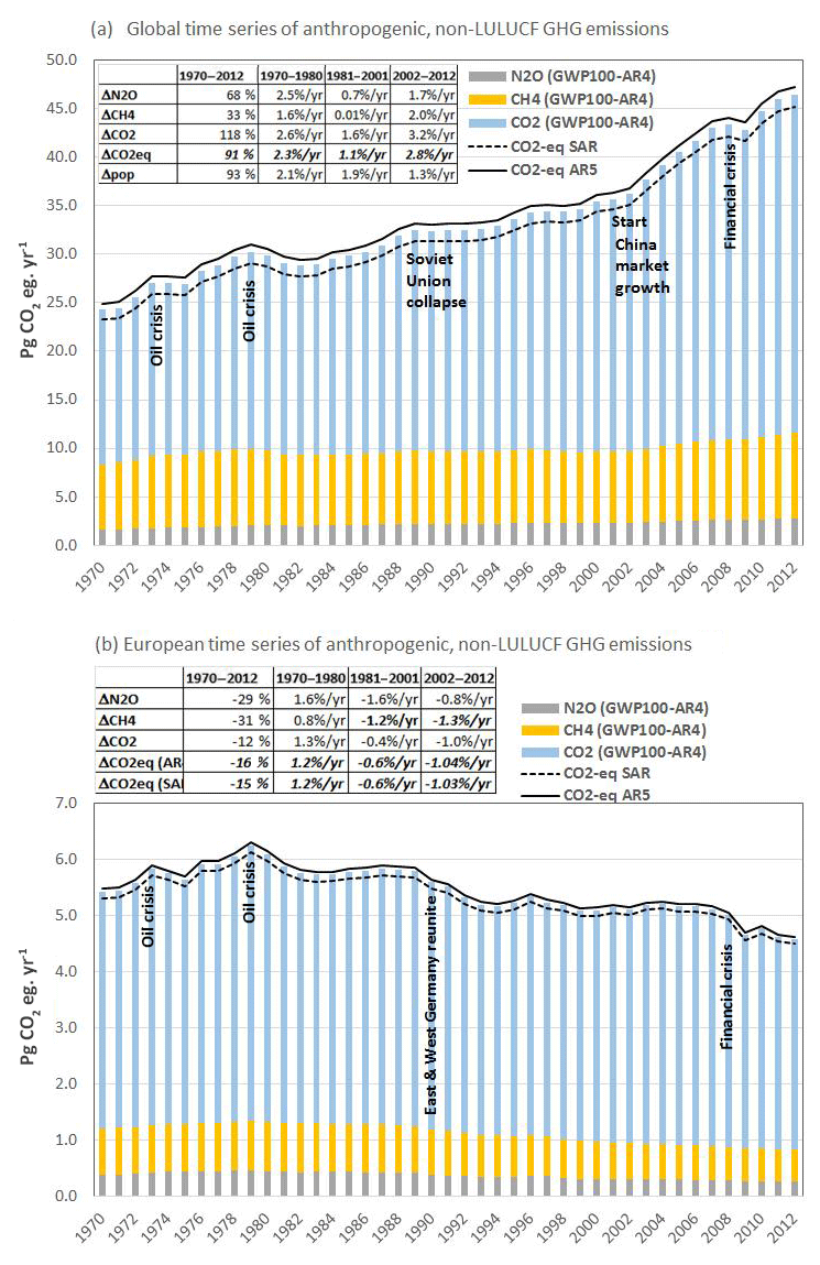
Figure 3Time series 1970–2012 of fossil fuel CO2, CH4 and N2O global emissions from human activities excluding the LULUCF sector with global total (a) and European total (b). The stacked bars use AR4 GWP-100 values, whereas the dashed line and full line indicate the total CO2eq of the three gases in the case where the SAR and AR5 GWP-100 values are respectively used.
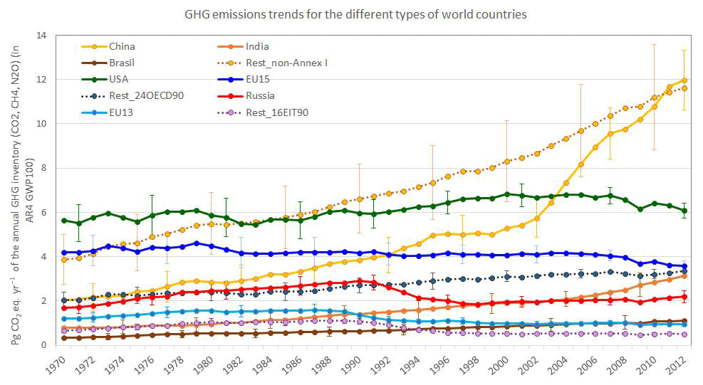
Figure 4Annual greenhouse gas time series 1970–2012 of EDGAR v4.3.2 with periodic error bar indication for the different types of countries with top emitters: (i) non-Annex I countries with China, India, Brazil and the rest of the non-Annex I countries, (ii) 24OECD90 countries with USA, EU15 and the remaining eight OECD countries of 1990, and (iii) 16EIT90 countries with Russia, EU13 and the remaining two newly independent Eurasian states. For the figures per gas we refer the reader to Fig. S4a–c.
3.2 The global CH4 budget
Table 4 compares the EDGAR v4.3.2 global CH4 estimates of 0.34(±0.16) Pg CH4 yr−1 with four other global datasets (the bottom-up inventories of US EPA, 2012, and GAINS14 Eclipse v5 of Höglund-Isaksson, 2012); and the global budgets of Kirschke et al. (2013) and Saunois et al. (2016). Even though the global total CH4 emissions for the bottom-up inventories vary by less than 4 %, global annual emissions from the agricultural and fossil fuel production sectors vary with ±22 % and ±17 % respectively. The top-down inventory estimates are 16 %–29 % larger than the bottom-up ones.
Figure 7a illustrates the origin of the large variations in the estimated fugitive emissions of oil and gas production (including extraction, transmission and distribution). Large uncertainties in CH4 from venting and flaring at oil and gas extraction facilities have been reported by e.g. Lyon et al. (2015) or Peischl et al. (2015). The CH4 venting of oil and gas extraction facilities is, in particular during the times of the Soviet Union, now believed to be larger than previously thought (e.g. in EDGAR v4.2 or US EPA), after Höglund-Isaksson (2017) used ethane–methane ratios as indicators. Additionally, gas distribution is a relatively large source of uncertainty, in particular in countries with old gas distribution city networks using steel pipes now distributing dry rather than wet gas, with potentially more leakages. Based on IPCC (2006a), EMEP/EEA (2009, 2013) and Marcogaz (2013), the emission factors for steel and grey cast iron pipelines vary in the range of 0.1–7 t km−1 yr−1, whereas this is a factor of 2 lower for PVC and polyethylene pipelines. The difference in composition of the gas distribution networks is taken into account in EDGAR v4.3.2 with country-specific variations in emission factors. The high CH4 emissions during the natural gas transmission in the Russian reporting to UNFCCC (2016) might also account for all or part of accidental CH4 releases, which are not negligible according to Höglund-Isaksson (2017). These are not included in the EDGAR datasets.
China is currently the top emitter of CH4 because it has become the largest coal producer and it is a major rice cultivator. While the fugitive CH4 emissions from coal production in China are increasing, emissions from rice cultivation are decreasing, as shown in Fig. 7b. The emission factor CH4 ha−1 yr−1 for irrigated rice fields has been reduced from 1970 to 2000 by by changing farming practices, as reported by Li et al. (2002), resulting in 0.47 kg CH4 ha−1 yr−1 for the last decade. A comparison with Peng et al. (2016) illustrates the large range of emission factors used: the emission factor in EDGAR v4.3.2 for rice cultivation is twice as high as in Peng et al. (2016). Also for the coal mining the CH4 emission factor for China in EDGAR v4.3.2 is 9 % higher than in Peng et al. (2016). EDGAR v4.3.2 revised emission factors for coal mining with local data from Peng et al. (2016), weighted by coal mine activity per province. These emission factors are at the lower end of IPCC (2006c) recommendations and yield EDGAR v4.3.2 estimates of 17.2 Tg in 2008 and 21.2 Tg in 2012, which are comparable to estimates of Peng et al. (2016) within ±2 Tg.
Total CH4 emissions in EDGAR v4.3.2 in 2005 are 2 % (3 %) lower than in the v4.2 (4.1) version, which has been used in global inverse modelling studies of Monteil et al. (2011), Bergamaschi et al. (2013, 2015, 2018), Ganesan et al. (2015), Kort et al. (2008), and Miller et al. (2013). Except for the Chinese coal mining, no other major shortcomings to v4.2 were indicated in these global studies. More regional inverse modelling studies are nowadays able to “verify”15 the CH4 emissions better (such as Henne et al., 2016, for Switzerland), and first atmospheric model runs with EDGAR v4.3.2 CH4 emissions started recently. Total emissions have not changed significantly for either EU28 or the USA, but there are changes in the patterns of emissions: the −2.5 % (−0.2 %) change in the EU28 estimates of v4.3.2 compared to those of v4.2 (v4.1) is still within the range of the inverse model simulations of Bergamaschi et al. (2018), while the −4.7 % (−3.4 %) change in the USA in EDGAR v4.3.2 compared to v4.2(v4.1) is not in line with the suggested +50 %–70 % higher anthropogenic emissions based on the inverse modelling study of Miller et al. (2013). The latter might be explained on the emissions side by delayed reporting of statistics on fracking for shale gas and oil and the not well-characterised and highly uncertain emission factors as indicated by the US EPA (2015) and on the modelling side by large uncertainties in inverse models and the potential contribution of natural sources. For China the EDGAR v4.3.2 estimate for fugitive emissions from coal mining yields a 38 % lower CH4 emissions total in 2008, which is in line with Saunois et al. (2016), Brandt et al. (2014) and Kirschke et al. (2013), suggesting lower CH4 emissions in particular in northern China where coal mining takes place.
3.3 The global N2O budget
An overview of the global N2O budget is not yet available as for CO2 and CH4. Recent efforts from the modelling community to provide input for the global N2O budget by Tian et al. (2018) report anthropogenic emission estimates for 2006 of 10.8 Tg N2O yr−1, confirming the 2005 global total by US EPA (2012) of 10.9, but a full overview of the global nitrous oxide budget is still forthcoming. The bottom-up estimate of EDGAR v4.3.2 of 7.2(±3.7) Tg N2O yr−1 for 2005 differs from this with 34 %, which is still within the uncertainty range. The bottom-up estimate of GAINS by Winiwarter et al. (2018) differs in a similar way by 29 %. It is noted that the differences within each source category remain very large (see Table 5). A comparison at European level between EDGAR v4.3.2 and the N-budget of Leip et al. (2011) shows relative moderate discrepancies also at sector-specific level for the total and agricultural sectors, 26 % or 37 % smaller estimates by EDGAR compared to Leip et al. (2011), but for the non-agricultural sectors, 19 % larger estimates. Höglund-Isaksson et al. (2010) provided GAINS estimates for EU27 that are respectively 28 %, 42 % and 20 % larger than the total, agriculture and non-agricultural sector estimates of Leip et al. (2011).
Although in EDGAR v4.3.2 the agricultural sector contributes most to the anthropogenic direct and indirect N2O emissions, the production of chemicals, such as nitric acid, glyoxal, caprolactam and adipic acid, and its use as anaesthesia or for aerosol spray cans also play an important role. In 1970 the chemicals sector contributed 20 % to the total, but this has been significantly reduced to less than 8 % because of technological developments. Figure 8 shows the impact of technological developments from old plants to higher-pressure plants or plants with non-selective catalytic reduction, reducing the N2O emissions by factors of 2 and 10 respectively. The N2O emissions of nitric and adipic acid plant facilities which EDGAR v4.3.2 estimated are in line with the estimates of US EPA (2012) and by GAINS for the year 2005. However, a discrepancy evolves when looking at the 2010 values, because of the relatively large reduction between 2007 and 2010 in EDGAR and the relative constant trend in GAINS. While EDGAR assumes abatement technologies for nitric and adipic acid plants in China following the reporting under the Clean Development Mechanism, Schneider et al. (2010) assume that abatement was not used at least for the new adipic acid plants. The latter assumption was followed by Winiwarter et al. (2018) and explains the differences in the global nitric and adipic acid N2O emission estimates between GAINS and EDGAR.
4.1 Global greenhouse gases 1970–2012
A country-based statistical analysis including 4 decades of GHG emissions (EDGAR v4.2) and GDP (Purchasing Power Parity data of the Penn World Tables 7 of Feenstra et al., 2013) was carried out to investigate the possible causality between emissions and income. The results, summarised in Paruolo et al. (2015), showed that no presence of causality could be statistically proven. This reflects a complex link between the very heterogeneous economic activities (ranging from manufacturing to services) and emissions, and justifies the meticulous bottom-up inventory compilation using statistics instead of modelling.
Figure 3 shows the global trend of GHG emissions in CO2 equivalent (100-year time horizon), using the GWP-100 values of AR4 (IPCC, 2007)16. The GHG total is composed of all sources (excluding LULUCF) of CH4 and N2O but only CO2 from long-cycle C fossil sources and excluding the short-cycle17 C for the CO2 accounting, conforming to IPCC (2006a). The estimated global total GHG in 2010 of 44.7 Pg CO2eq was shown to be 0.7 % lower than the estimates for the 2010 global total (without LULUCF) in the UNEP (2012, 2015) Emission Gap reports. The share of each gas to the total GHG is relatively stable and yields for CO2 76.8 % (+2.1 pp, −1.2 pp), for CH4 18.1 % (−2.5 pp, +1.9 pp) and for N2O 5.1 % (+0.4 pp, −0.6 pp), where in between brackets the percent point impact of the evolution of the GWP-100 value from the SAR (IPCC, 1996b)18 to the AR5 (IPCC, 2014)19 is given.
In the global GHG emissions time series, the trend was shown to be dominated by CO2 as it has the largest share and the largest increase. In the 1970s N2O increased at the same rate as CO2 (2.6 % yr−1), while CH4 was half as fast. In the 1980s and 1990s, N2O and CH4 increases were very small, while CO2 continued albeit at a slower rate (1.6 % yr−1). In the last decade, 2002–2012, CO2 and CH4 growth rates increased with respectively 3.2 % yr−1 and 2.0 % yr−1. While over the 4 decades (1970–2012) the global total GHG increased in line with global population (91 % versus 88 %), the inter-annual and regional emission variations do not always reflect the rates in population increase, but are instead better explained by the global fuel markets and economy, the 1973 and 1979 oil crises, the dissolution of the Soviet Union (1989–1991), the growth of the Chinese economy, after they joined the World Trade Organisation in 2002, and the 2008 global financial crisis.
4.2 Greenhouse gas trend analysis for regions and top emitting countries
Figure 4 shows the GHG trends for the major regions: 24OECD90 (split into USA, EU15 and the rest), 16EIT90 (with Russia and EU13 and the rest) and non-Annex I (for which China, India and Brazil are shown separately). The gas-specific GHG trend is also available per country in Janssens-Maenhout et al. (2017) and is downloadable from https://edgar.jrc.ec.europa.eu/overview.php?v=CO2andGHG1970-2016. To understand the trends of the total GHG (in CO2eq), the decomposition with the trends of CO2, CH4 and N2O for the same regions is given in Fig. S4a, b and c respectively and with a discussion per country group in the Supplement.
Focussing on the top four emitting countries and regions, Fig. 5 compares the reported UNFCCC (2004, 2012, 2014, 2016, 2017) emissions of China, USA, EU28, and Russia and the emission estimates of EDGAR v4.3.2. There is a very good agreement between the UNFCCC-reported values and the EDGAR v4.3.2 estimates for the EU28, whereas for USA and Russia the EDGAR v4.3.2 estimates are lower than those reported by UNFCCC (2016). For the USA this is explained by lower N2O emissions in EDGAR v4.3.2, although N2O emissions reported by USA to UNFCCC (2014, 2016) are within the large uncertainty range for the EDGAR v4.3.2 estimates. For Russia CH4 emissions reported to UNFCCC (2016) are 37 % higher than those estimated by EDGAR v4.3.2, but this is also within the uncertainty range. The largest difference is found in the estimation of gas pipeline transmission emissions, which are 4 times higher in the UNFCCC inventory of Russia than in EDGAR v4.3.2. The relatively low emission factor for gas pipelines, used by EDGAR, is in line with the recommendations of Lelieveld et al. (2005). For China, a very good agreement between the EDGAR v4.3.2 estimate and the UNFCCC (2004, 2012, 2017) reported values is obtained, taking into account the importance of the coal statistics revision. In order to evaluate the latter effect, two time series of emission are calculated by EDGAR, with and without coal statistics revision. The revision includes a decrease in the 2010–2012 values and yields an increase for the 1990–2009 values of about +3 % for 2005 and 1994. It is evident that the previous estimates of the UNFCCC inventory in 2005 and 1994 would need to be revised in order to evaluate the emissions change from 2005 to 2012. Even if relative uncertainty in EDGAR estimates for China could be reduced, it is evident that the size of the Chinese inventory has a large impact on the global absolute uncertainty.
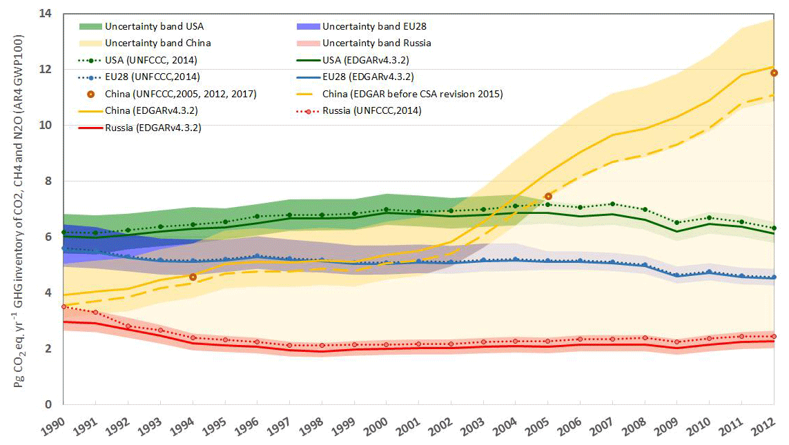
Figure 5GHG emissions of the largest emitting countries and regions (USA, EU28, Russia, China) of EDGAR v4.3.2 (solid line) with their uncertainty band compared to the reported UNFCCC time series of 2016 (dotted line). For China, two inventories were reported by national communications (1994, 2005), and a biennial update in 2017 added a new inventory value for 2012. The dashed yellow line gives the EDGAR v4.3.1 estimate of the Chinese GHG emissions using the energy statistics before the Coal Statistics Abstract (CSA) revision of October 2015.

Figure 6Intercomparison of CO2 emissions trends estimated by EDGAR and by others with (a) details for cement process emissions globally with data of Le Quéré et al. (2016) and Xi et al. (2016), and (b) details for China's sector-specific emissions with data of Guan et al. (2012) and Liu et al. (2015). The total is for all datasets subdivided into fossil fuel combustion and industrial process emissions (i.e. non-combustion industrial emissions, including cement).
In this section, the gridded EDGAR datasets at are further screened to identify hot spots and to check for anomalies. An overview of the region-specific totals and their sector-specific composition for the year 2012 is given in Figs. 9, 12 and 15 for the different substances. The sector-specific country totals are provided in the overview Table 6a per region and Table 6b per sector for 2012.
Table 6(a) Global and regional GHG emissions (in Gg and tons per person) for the year 2012. CO2eq emissions have been calculated including only CO2 from long-cycle carbon only, CH4 and N2O. (b) Global sector-specific GHG emissions for the year 2012 (in ktons and tons per person). CO2eq emissions have been calculated including only CO2 from long-cycle carbon only, CH4 and N2O.
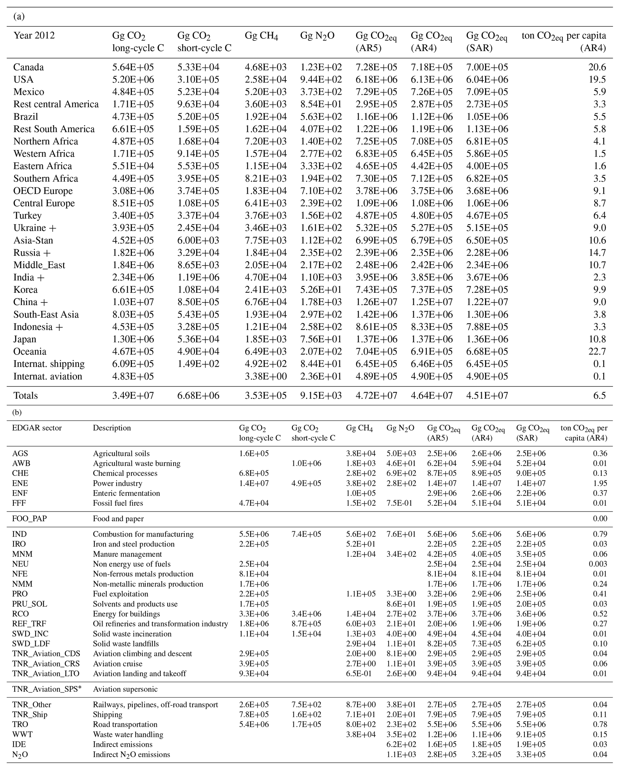
* Note that emissions from the Supersonic aviation are available only till the year 2003, when the Concorde airplanes stopped flying.
5.1 CO2 emissions and urban hot spots
The 2012 grid map of CO2 emissions from both long-cycle and short-cycle carbon in Fig. 9 with the relative sectorial breakdown for selected world regions (Europe, North America, Latin America, Africa, Middle East, Oceania, Russia and China) clearly shows the fossil fuel combustion activities, representing 90.6 % of the total CO2 emissions. In this section we include for completeness biofuel emissions, which were omitted from the comparisons with UNFCCC reporting, because UNFCCC assumes carbon neutrality for all agricultural and biofuel CO2 emissions in a country for any individual year. In the 24OECD90 countries 75.2 % of CO2 emissions are produced by the power, road transport and residential sectors, while these sectors represent only 60.9 % in non-Annex I countries. The share of the industrial combustion and production sectors (mining/manufacturing) of non-Annex I countries reaches 36.8 %. The CO2 shares of the fuel combustion in the power generation, road transport, buildings and manufacturing sectors vary for the different regions from 16 % to 50 %, from 5 % to 27 %, from 6 % to 39 % and from 9 % to 22 % of total emissions (see Table 6a and b) respectively. Interestingly, agricultural waste burning20 represents 10 % of CO2 emissions in Latin America (mainly due to sugarcane crop residue burning), and 22 % of CO2 emissions in Africa derives from the transformation industry (charcoal production using as input primary solid biomass). Industrial emissions are distributed at the point-source locations of the power/heat plants or industrial facilities (e.g. cement factories) using the capacity of the plants or facilities as a weighting factor.
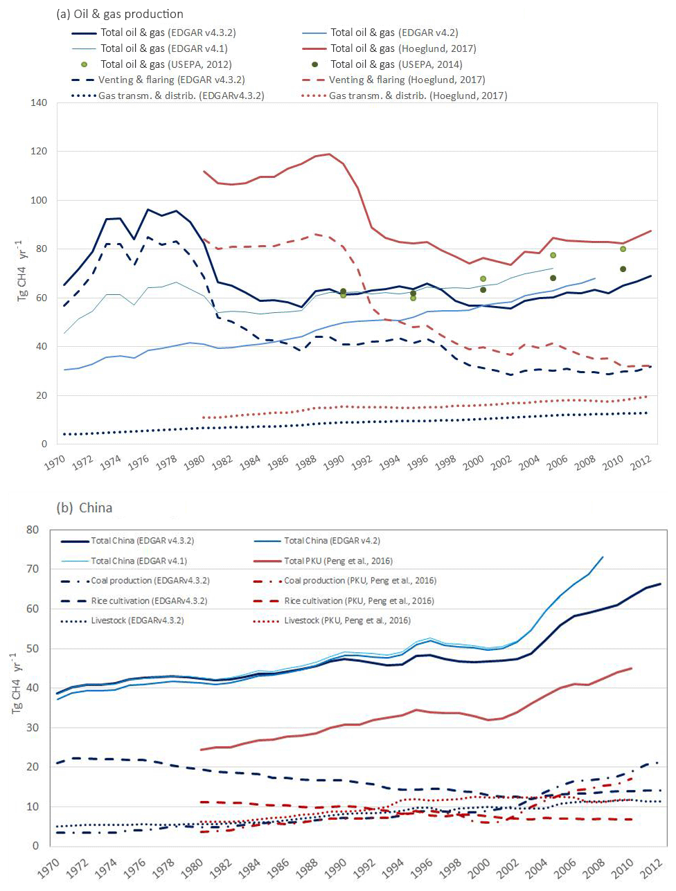
Figure 7Intercomparison of CH4 emissions trends estimated by different versions of EDGAR and by others with (a) details for the CH4 venting for oil and gas extraction, transmission and distribution with data of Höglund-Isaksson (2017) and (b) details for China's sector-specific emissions with data of Peng et al. (2016).
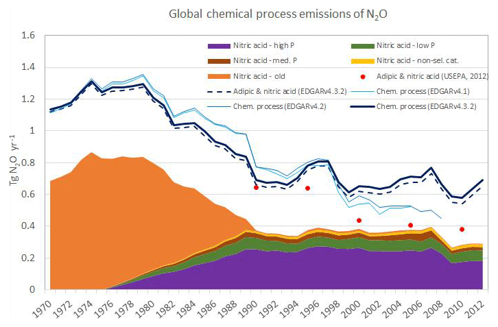
Figure 8Global N2O emissions trends for chemical processes, which mainly originate from nitric and adipic acid production (apart from smaller contributions from glyoxal and caprolactam production). The coloured area illustrates the penetration of technology for nitric acid production (with high-pressure plants, medium-pressure plants, low-pressure plants, plants with non-selective catalytic reduction and old plants) to reduce the emissions.
In the grid maps hot spots are particularly visible over cities, of which the top four emit 2.75 % of the global total21 and coincide with the cities of Shanghai, Huangshi, Shenyuang and Moscow. In fact, 5 % of the grid cells emit more than 5 Mt yr−1 and account for 34.08 % of the global total. It is therefore interesting to look at the contribution of the various sectors in megacities, as shown in Fig. 10. Emissions from the road transport sector (Fig. 10a) for the 20 selected cities seem to be more important in suburban areas than in the centre of the megacity. For power plants more heterogeneity was found (Fig. 10b), with larger power plants typically located on the periphery of the city in the 24OECD90 countries, while for major cities of the 16EIT90 and non-Annex I countries, several larger power plants are located within the central city areas. The remaining share of CO2 emissions was shown to be mainly from the building sectors and the industrial manufacturing emissions.
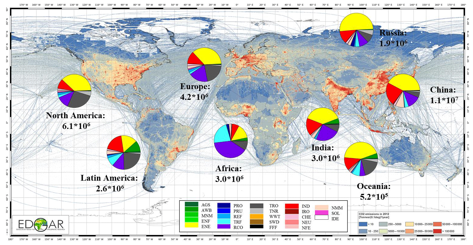
Figure 9CO2 emission grid map and relative contribution of EDGAR sectors in world regions (pie charts) for 2012. The legend for the PIE charts relates to the EDGAR sectors defined in Table S3: AGS: agricultural soils, AWB: agricultural waste burning, MNM: manure management, ENF: enteric fermentation, ENE: power industry, PRO: fuel production, PRU: production and use of products, REF: oil refineries, TRF: transformation industry, RCO: residential, TRO: road transport, TNR: non-road transport, WWT: waste water, SWD: solid waste disposal, FFF: fossil fuel fires, IND: manufacturing industry, IRO: iron and steel, CHE: chemicals, NEU: non-energy use, NFE: non-ferrous metals, NMM: non-metallic minerals, SOL: solvents, IDE: indirect emissions. The represented CO2 emissions also include those from short-cycle carbon (i.e. of e.g. biofuel combustion and agricultural waste burning).
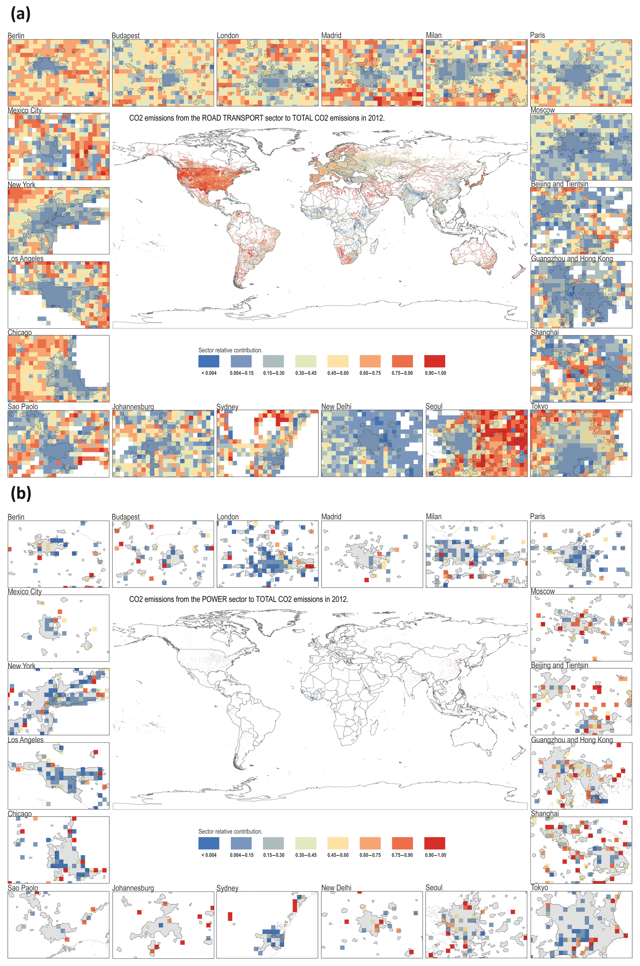
Figure 10(a) Zoom of CO2 emission grid maps over cities, representing the share of the road transport within the cities. The represented CO2 emissions also include those from short-cycle carbon. (b) Zoom of CO2 emission grid maps over cities, representing the share of the power plants within the cities. The represented CO2 emissions also include those from short-cycle carbon.
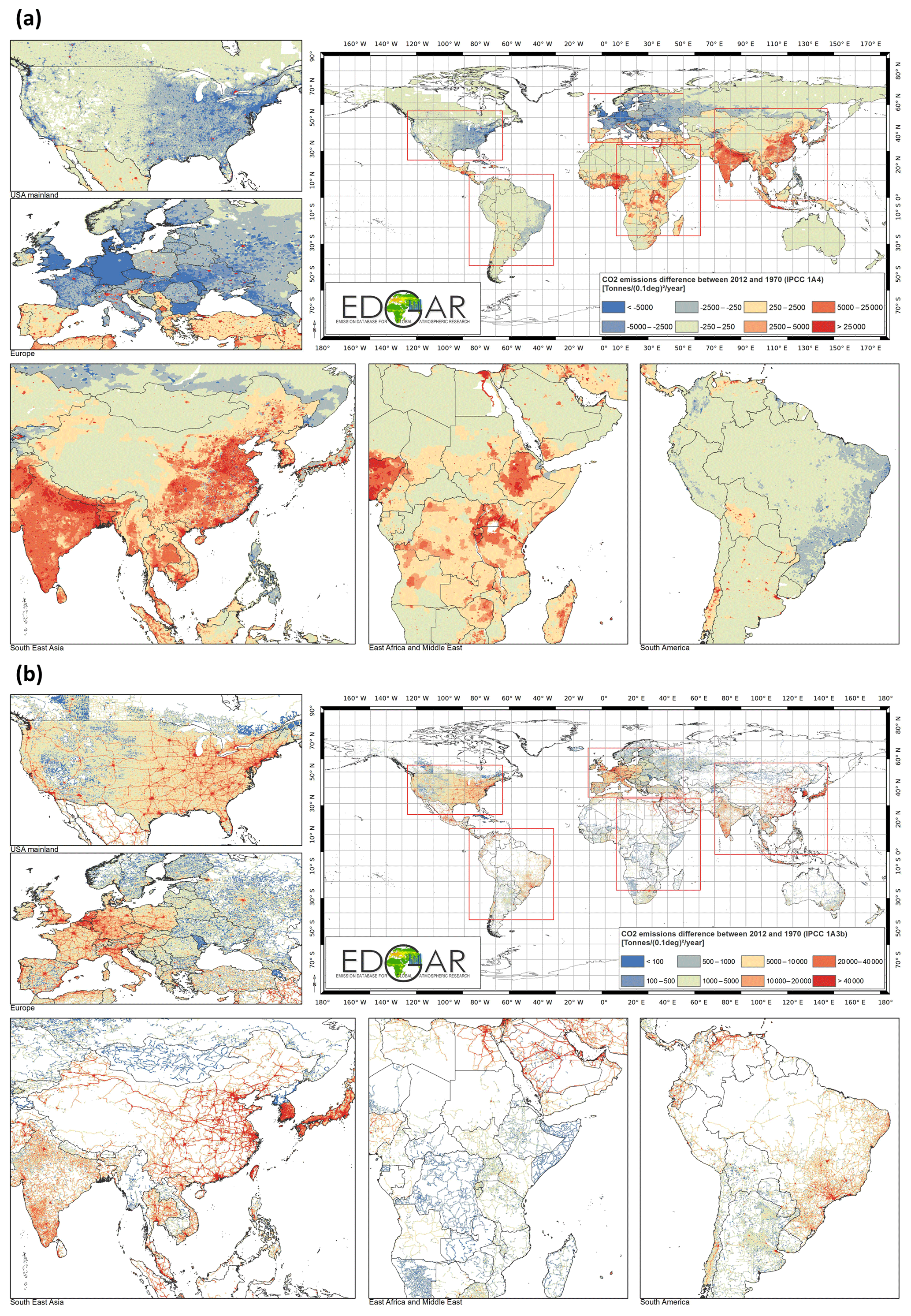
Figure 11(a) Difference in CO2 emissions from buildings between 2012 and 1970. The represented CO2 emissions also include those from short-cycle carbon. The figures for the long-cycle and short-cycle carbon separately are taken up in Fig. S5. (b) Difference in CO2 emissions from transport between 2012 and 1970. The represented CO2 emissions also include those from short-cycle carbon. The figures for the long-cycle and short-cycle carbon separately are taken up in Fig. S5.
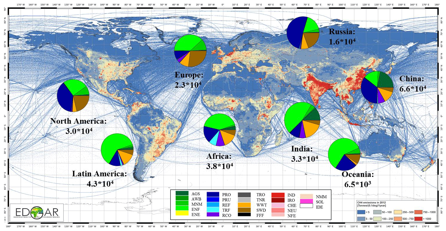
Figure 12CH4 emission grid map and relative contribution of EDGAR sectors in world regions (pie charts) for 2012. The legend for the PIE charts relates to the EDGAR sectors defined in Table S3: AGS: agricultural soils, AWB: agricultural waste burning, MNM: manure management, ENF: enteric fermentation, ENE: power industry, PRO: fuel production, PRU: production and use of products, REF: oil refineries, TRF: transformation industry, RCO: residential, TRO: road transport, TNR: non-road transport, WWT: waste water, SWD: solid waste disposal, FFF: fossil fuel fires, IND: manufacturing industry, IRO: iron and steel, CHE: chemicals, NEU: non-energy use, NFE: non-ferrous metals, NMM: non-metallic minerals, SOL: solvents, IDE: indirect emissions.
The evolution over time from 1970 to 2012 shows a different pattern for the residential sector than for the road transport sector. Figure 11a shows that while the residential sector decreased over these 4 decades in America and Europe, it increased in Asia and Africa. The difference in CO2 emissions from the road transport sector meanwhile presents in Fig. 11b a more homogeneous picture with increases from 1970 to 2012 in almost all regions. Please note that Fig. 11 includes both long-cycle and short-cycle carbon fuel use, but Fig. S5a–d presents these separately and shows e.g. the use of the vegetal waste and dung for residential heating in India and the biofuel use for car transport in Brazil.
5.2 CH4 emission maps
Because CH4 is mainly released from fermentation processes (enteric, manure, landfills or rice) or diffusion processes (coal mine leakage or gas distribution losses), the 2012 CH4 emission grid map with sector contributions for major world regions (Fig. 12) does not mirror the same human activities as the CO2 map. The CH4 shares for enteric fermentation, fossil fuel production and transmission, and solid and water waste treatment range from 9 % to 59 %, from 8 % to 68 % and from 11 % to 37 % of the global total respectively, depending on the region. For 24OECD90 countries enteric fermentation (with 31.1 % share), fossil fuel production (28.1 %) and landfills (21.4 %) are the three dominant sectors, whereas in the 16EIT90 countries, CH4 emissions are dominated by fossil fuel production (49.4 % share). The non-Annex I countries show a similar high share of enteric fermentation and fossil fuel production to the 24OECD90 countries, but rice cultivation and domestic wastewater together give much higher emissions than solid waste disposal. Rice cultivation was shown to contribute significantly to the total CH4 inventory of China (21.5 % or 14.2 Tg in 2012), which is almost 11 times the CH4 emissions of rice cultivation in India (3.8 Tg), despite the larger area for rice fields in India than in China (425 000 compared to 303 000 km2). This is explained by the fact that India typically has one harvest per year from 1∕3 rain-fed fields and 2∕3 irrigated fields, whereas China has multiple harvests per year from irrigated rice fields. Rain-fed rice fields in India are modelled with a 5 times lower emission factor than the irrigated fields in China. Figure 13a and b show the opposing trends with mainly positive 2012–1970 increments in enteric fermentation (mainly cattle) (a) and mainly negative increments in CH4 emissions from rice cultivation (b). The CH4 trend from rice cultivation in Asia was shown to be remarkably stable, with the exception of Thailand, where increased activity is noticed. The remaining non-Annex I countries of Africa and Latin America show similar high contributions from enteric fermentation (25.8 Tg versus 20.9 Tg respectively in 2012). However, the total CH4 emissions from the African continent are higher than those of Latin America because of the 3.5 times larger CH4 emissions from fossil fuel production (gas and oil production). Interestingly, both continents show significant CH4 emissions from charcoal production, which compares to 16 % (Africa) and 15 % (Latin America) of their gas and oil production emissions of CH4.
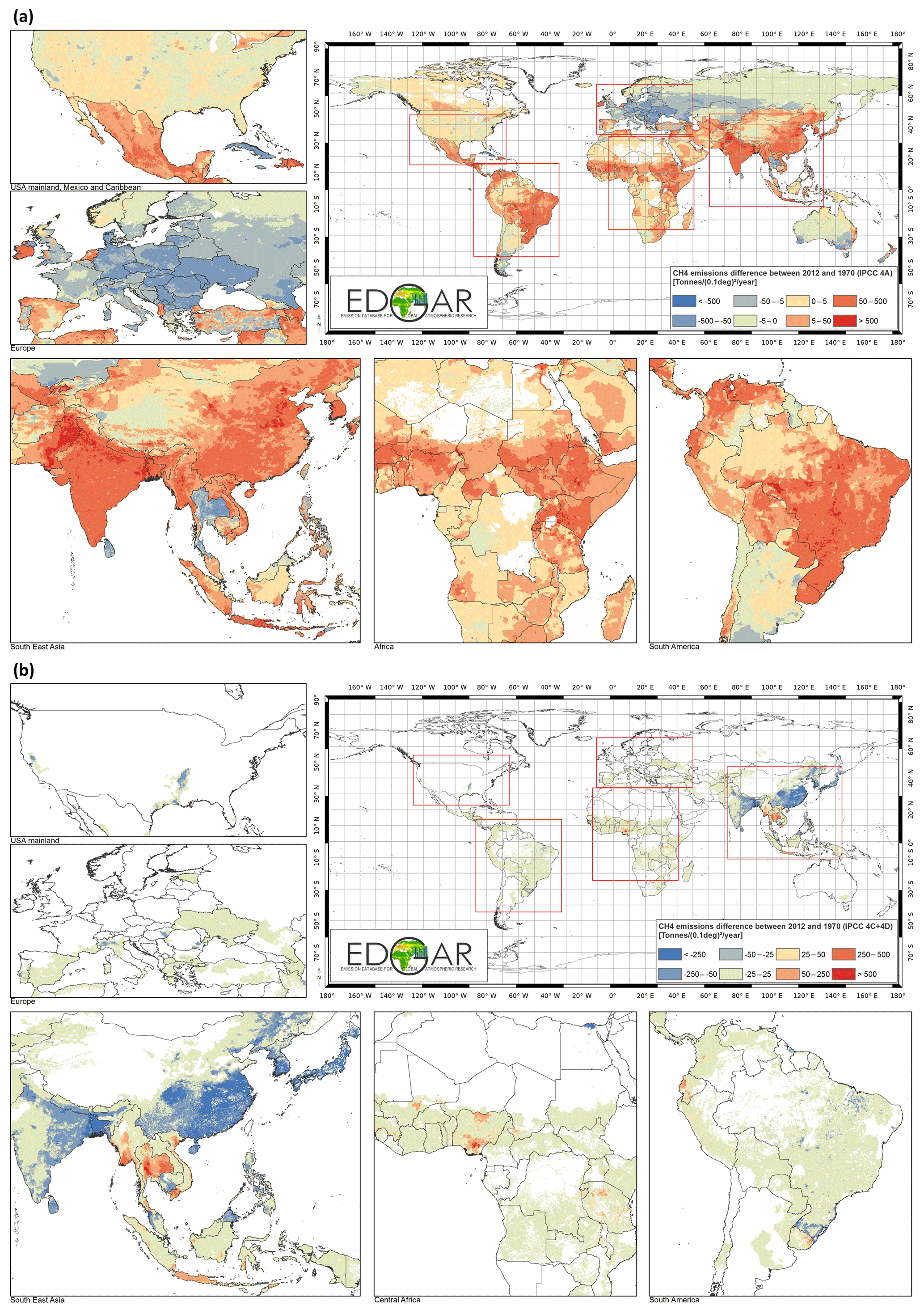
Figure 13(a) Difference in CH4 emissions from enteric fermentation between 2012 and 1970. (b) Difference in CH4 emissions from rice cultivation between 2012 and 1970.
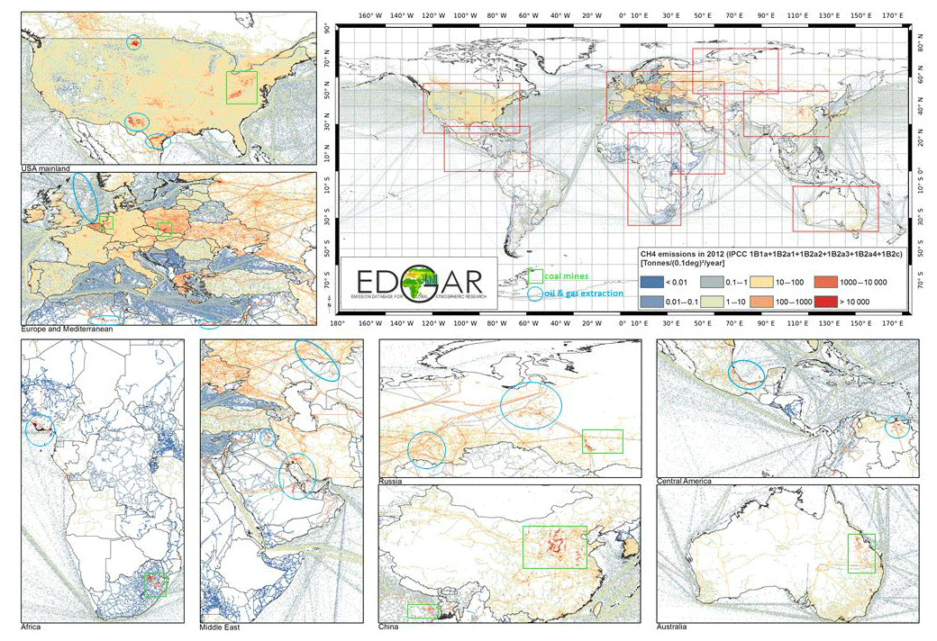
Figure 14CH4 emissions from fossil fuel production in 2012 with zoom on areas with intense coal mining (within green frame) and gas and oil production activities with venting (within blue circle). The shipping lines are representing the CH4 leakage during transmission of oil tanker transport as fugitive emissions from the fuel and not as combustion emissions from the tanker.
Hot spots of CH4 are estimated for fossil fuel production, typically at gas and oil production facilities or at coal mines, as shown in Fig. 14. In North America a shift over the period 2005–2012 from coal mining in the north-east (−21 %) to gas and oil production in particular in North Dakota, Montana and Texas (+65 %) took place. The USA is nowadays the largest producer of both shale gas and tight oil, which make up almost half of total US gas and oil production (EIA, 2015). In Europe a much larger decrease of −87 % in coal production happened earlier, while gas production increased by 30 %. Consequently the EU28 needed to rely on oil and gas imports and expanded its transmission and gas distribution network, with a corresponding increase in CH4 leakages. Apart from the USA, the Middle East was also shown to be a global world player on the oil and gas market, shifting from oil production (with a decrease of 71 % over the period 1976–1985) to gas production (with a 9.3-fold increase from 1985 to 2012), mainly driven by Iran, Saudi Arabia and Qatar. The African countries with the highest CH4 emissions from fossil fuel production were in decreasing order of importance Algeria and Nigeria (for oil and gas production) and South Africa (for coal mining). Similarly to Nigeria, which showed an approximate doubling of CH4 emissions from oil (and gas) production over the last 4 decades, Mexico and Venezuela also showed similar levels of CH4 emissions from oil and gas production (increasing by a factor of 1.6 over the 4 decades). For gas production, Russia has shown the largest CH4 venting and leakage, overtaking the USA in 1985.
Coal mining has become important for China, which since 1982 has been the largest bituminous coal producer in the world, overtaking the USA. Moreover, China was shown to also be the largest coal importer since 2011 (overtaking Japan), as domestic coal produced in mainly the western and northern inland provinces of China faced a bottleneck in transportation, lacking southbound rail lines (Tu, 2012) towards the southern coast that has the highest coal demand. Not only did EDGAR v4.3.2 revise the country-specific coal mining emission factors, but the spatial distribution was also considerably updated with hot spots at the location of the mining activity. For coal mine activities in China (split into brown and hard coal), the coal mine database of Liu et al. (2015) provided over 4200 coal mine locations, which is 10 times more than that available for EDGAR v4.2. For Europe, the closure of mines since the 1990s has been taken into account using the European Pollutant Release Transfer Register (EPRTR, 2012).
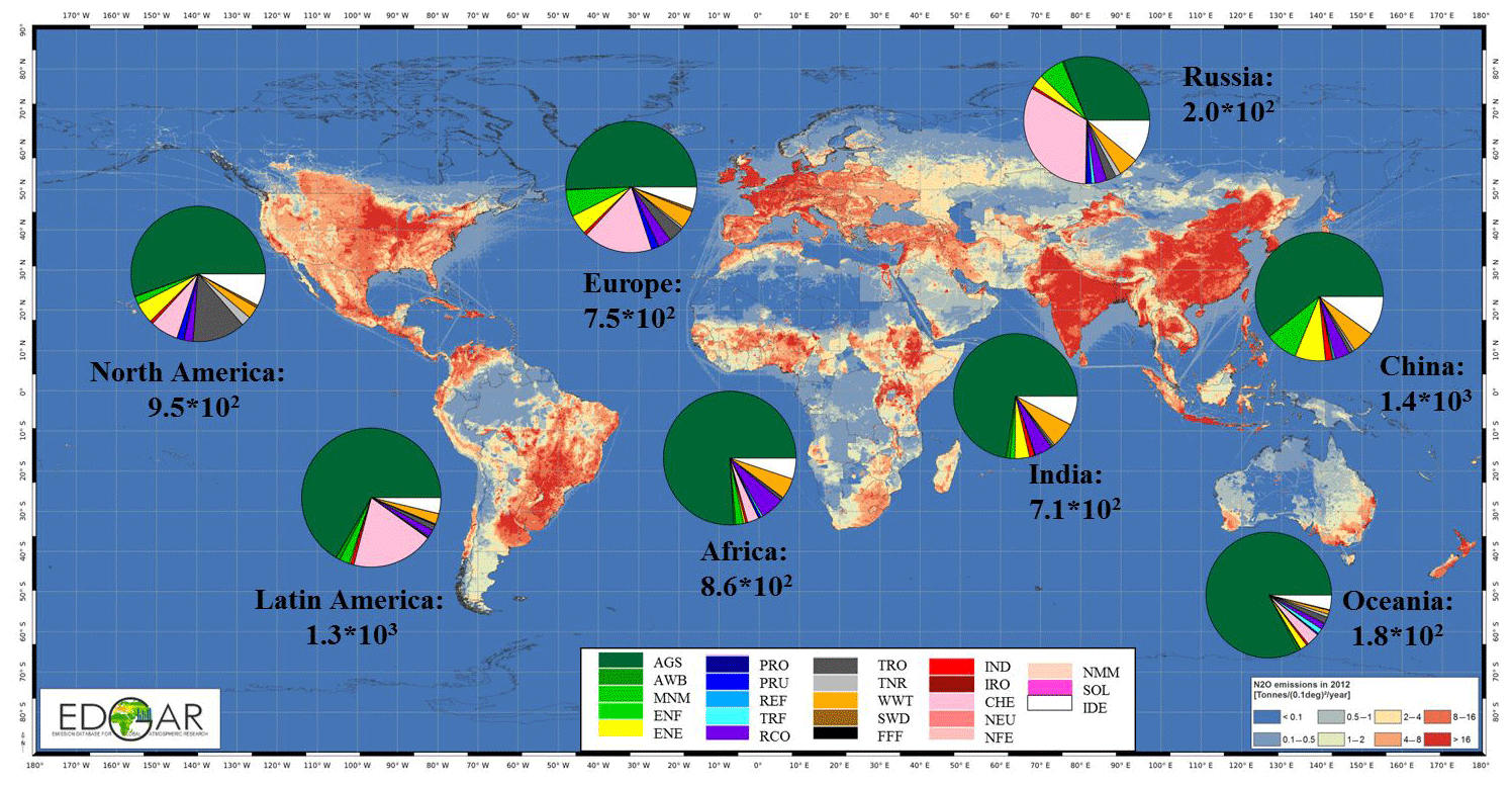
Figure 15N2O emission grid map and relative contribution of EDGAR sectors in world regions (pie charts) for 2012. The legend for the PIE charts relates to the EDGAR sectors, defined in Table S3: AGS: agricultural soils, AWB: agricultural waste burning, MNM: manure management, ENF: enteric fermentation, ENE: power industry, PRO: fuel production, PRU: production and use of products, REF: oil refineries, TRF: transformation industry, RCO: residential, TRO: road transport, TNR: non-road transport, WWT: waste water, SWD: solid waste disposal, FFF: fossil fuel fires, IND: manufacturing industry, IRO: iron and steel, CHE: chemicals, NEU: non-energy use, NFE: non-ferrous metals, NMM: non-metallic minerals, SOL: solvents, IDE: indirect emissions.
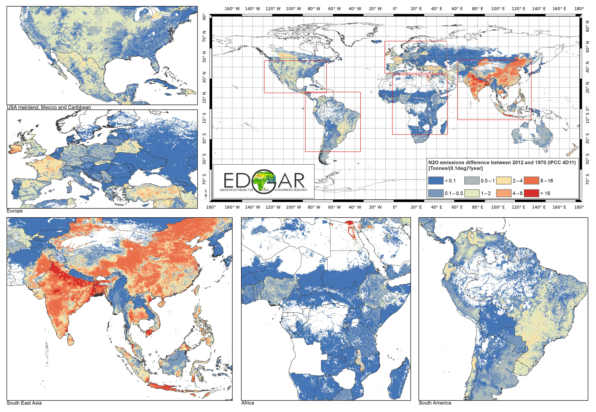
Figure 16Difference between 2012 and 1970 in N2O emissions from fertiliser use on agricultural soils.
5.3 N2O emissions including indirect sources
Unlike the CO2 and CH4 grid maps, the gridded N2O emissions for the year 2012 in Fig. 15 with the share of different sectors for world regions showed a quite uniform global coverage distribution, due to the predominance of soil emissions and indirect emissions (distributed with the N-deposition map of Dentener et al., 2006), also from the sea's surface. Over land, most N2O is emitted from the agricultural soils (the use of animal manure as fertiliser, the application of N-containing fertilisers and cattle in pasture), representing 35 % to 86 % of total N2O emissions depending on the region. Fertilising farmland with pasture or animal waste as fertiliser or crop residues has not increased so much as the use of nitrogen fertilisers. Figure 16 shows the increased use (by the difference 2012–1970) of nitrogen fertiliser, in particular in Asia.
Annual grid maps for all GHGs and sectors covering the years 1970–2012 are available as txt (expressed in the unit ton substance per grid cell) and NetCDF (expressed in the unit kg per substance m−2 s−1) with spatial resolution, available under https://doi.org/10.5281/zenodo.2658138 (Janssens-Maenhout et al., 2019). (This is the GHG part with CO2, – long-cycle carbon, CO2 – short-cycle carbon, CH4 and N2O grid maps and time series of the EDGAR dataset with PID: http://data.jrc.ec.europa.eu/dataset/jrc-edgar-edgar_v432_ghg_gridmaps.) In addition, monthly GHG global grid maps are produced for 2010 and are available per sector and substance. The main features of the grid maps are described (Sect. 5) while focusing on the year 2012, although analogous considerations also pertain to previous years.
In line with the ESSD guidelines of Carlson and Oda (2018), we aim with this publication not only for free open access to all calculated data (with their uncertainty), but also for a complete documentation of the EDGAR v4 products that has been compiled in a transparent way to the extent possible.
7.1 Strengths and applications of EDGAR v4.3.2
The EDGAR v4.3.2 scientific global emission inventory database provides a comprehensive dataset of anthropogenic emissions of CO2, CH4 and N2O in time series 1970–2012 (with monthly resolution) and spatially disaggregated grid maps with resolution. An advantage of EDGAR v4.3.2 is that the bottom-up emissions calculation methodology is applied to all countries and the results are available with regular updates based on a robust statistical data infrastructure and provide direct information to policy makers in the standard structure as used for the Annex I countries. EDGAR v4.3.2 may provide useful information to countries with less strong statistical data infrastructure for their future inventory requirement. In particular, the time series of EDGAR v4.3.2 can complete the emission trends for non-Annex I countries, as illustrated for the case of China, where the coal statistics revision also impacts the 2005 and 1994 inventory with +3 %.
For the atmospheric modelling community EDGAR v4.3.2 enables models to use historical emission grid maps for a top-down assessment of the total budget, making use of in situ and remote sensing atmospheric observation records. The results of inverse atmospheric models provide an evaluation of the nationally collected emission data with regard to their uncertainty and as such support the scientific review and updates of emission inventory methodologies. For recent years (e.g. 2010) total anthropogenic budgets of 33.6(±5.9) Pg CO2 yr−1, 0.34(±0.16) Pg CH4 yr−1 and 7.2(±3.7) Tg N2O yr−1 are obtained. The current evaluation capacity of inverse models using atmospheric measurements remains limited where the models struggle with an accurate separation of the natural emissions component from the total. Although modelling uncertainties and the uncertainties of natural emissions remain large, the atmospheric models provide observationally constrained top-down input, and it is expected that inverse models will increasingly contribute to the independent verification of the total fluxes. Moreover, the impact of updates of recommended tiered emission factors (such as from IPCC, 1996a, 2006a, the refinement of 2019, or selected region-specific data) on the resulting emissions can be assessed at global scale. EDGAR v4.2 evaluated the impact of the update of the N2O emission factor for direct soil emissions from the use of fertilisers (synthetic or manure or crop residues) by IPCC (2006c) with a 20 % lower value than what the IPCC (2000) Good Practice Guidance provided as a default. The update of the EDGAR v4.2 version to v4.3.2 demonstrated e.g. the necessity to take up region-specific emission factors for fugitive coal mining emissions in China, which are considerably lower than the IPCC lower tier-1 default values (e.g. Peng et al., 2016; Saunois et al., 2016).
With the 42-year long time series of EDGAR v4.3.2 we provide an important input to the analysis of global GHG trends. We find an accelerated increase in GHG emissions since the beginning of the 21st century compared to the 3 decades before, mainly driven by the increase in CO2 emissions from countries with emerging economies. For the EU-28 the trend is determined by a rather stable share of CO2 and a smooth but continuously decreasing CH4 contribution, resulting in an overall reduction of total GHG emissions. Even though the uncertainty of global total emissions has increased mainly because of the increasing share of GHG emissions from emerging economy countries, on a European scale the uncertainty has decreased because of the progress in inventory compilation and the decrease in some sectors with more uncertain CH4 emissions.
Overall the EDGAR v4.3.2 database aims at providing useful information for both the scientific and policy communities involved in understanding GHG emissions and budget, e.g. for the compilation of national inventories, the UNFCCC periodic global stocktake, analysis of co-benefits between air pollution and GHG emission mitigation strategies, interpretation of in situ or space-borne Earth observation data, or understanding and reducing of uncertainties.
7.2 Use, evaluation and limitation of the EDGAR v4.3.2 dataset
EDGAR v4.3.2 provides a global picture of GHG emissions using a tier-1–2 approach following IPCC (2006a) guidelines and allowing comparison of country- and sector-specific sources. This global completeness comes at the expense of lacking or less accurate information at (i) higher resolution or subnational focus and (ii) detailed modelling of subsector emissions beyond tiers 1–2.
Therefore, the potential users of the EDGAR v4.3.2 dataset are recommended to carefully consider these limitations when
-
applying it for region-specific, subnational or urban case studies, for which more detailed inventories should be used or constructed, using bottom-up and local information. EDGAR v4.3.2 only uses national data, and any subnational level is the result of a spatial distribution (top-down) making use of proxy data. In general large differences can be expected between the top-down spatially downscaled national emissions with proxy data and the bottom-up inventory with local data, sometimes not strictly reporting emissions that occur solely inside the small territory, as Gately and Hutyra (2017) demonstrate. The EDGAR v4.3.2 can be used to gap-fill between other regional inventories (e.g. in HTAPv2.2 of Janssens-Maenhout et al., 2015) or to bridge the gap between point sources and the national inventory (e.g. Theloke et al., 2011). These gap fillings come at the expense of losing consistency within the reported emissions as an inventory;
-
applying the dataset outside the period 1970–2012 can only be recommended when taking into account the fast track update from 2013 onwards based on recent statistics, for which we refer the reader to the annual publication on the hyperlink http://edgar.jrc.ec.europa.eu/index.php#. For the years before 1970 we refer the reader to the HYDE dataset. We would refrain from any linear extrapolation based on short-term trends of the emission time series or on emission drivers, for which the causality proof for these short time series is missing; and
-
comparing with other gridded datasets at grid-cell level, especially when using EDGAR v4.3.2 disaggregated subsector emissions data. Several assumptions about the technological evolution and the spatial distribution flow into the EDGAR v4.3.2 subsector emissions. The difference between two grid maps cannot be unambiguously attributed to missing activity data, the selected region-specific emission factor, or the assumed technology share or the spatial distribution proxy data. In particular, the latter factor is important, in particular for very localised sources or point sources (such as industrial complexes or urban areas). Moreover, the strength of point sources is very sensitive to the choice of the characteristic parameter (such as designed capacity or averaged annual emission estimate or given annual throughput) in the proxy dataset and can vary strongly over time. As Hogue et al. (2016) indicate, the largest uncertainty contribution in gridded emission datasets comes from the proxy data used for spatial disaggregration of national emissions. The subtraction of the sum of all the point sources from the sector-specific country total leaves a remaining emission that is composed of smaller sources and that is typically distributed with e.g. a population density proxy, as information is lacking. The uncertainties for the point sources and for the remaining smaller sources are highly different and larger than the uncertainty of the sector-specific country total. Information on the representativeness of the selected characteristic parameter for point sources is most critical and needs to be evaluated with measurements (such as in situ atmospheric measurements of co-emitted pollutants), but would require an in-depth analysis beyond the scope of this paper.
EDGAR v4.3.2 is the result of continuous improvement of previous datasets, which have been used by modellers in inverse modelling studies to verify the level and distribution of the emissions. Feedback has been taken into account (e.g. Saunois et al., 2017, for CH4). The evaluation of the dataset with a more advanced uncertainty assessment has not taken place yet.
7.3 Future perspective
EDGAR v4.3.2 demonstrates that inventories can be developed for all countries within the limitations of the quality of the available statistical data in order to contribute to the comprehensive picture needed for the UNFCCC periodic global stocktakes. In 2023 a first global stocktake is foreseen to track the progress of the collective efforts to reduce the emissions as promised under the Nationally Determined Contributions. Comprehensive information on emissions for all world countries can help to assess and build trust in the effectiveness of the NDCs. In particular, the country estimates of EDGAR v4.3.2 can help countries with less developed statistical infrastructures to compile their inventories and complete time series.
EDGAR v4.3.2 yields grid maps not only for all greenhouse gases, but also for air pollutants, representing multi-pollutant sources as single-point sources with realistic ratios of the different pollutant emission rates. To analyse the co-benefits and trade-offs of integrated approaches towards climate and energy as well as air quality policies, it is of key importance to use the transparency framework of “measuring–reporting–verifying” for a world-wide evaluation of the emissions. A bridge between the inventory compilers and satellite community can yield more dynamic emission databases. So far the interpretation of satellite data has been more successful with air pollutants, NOx, SO2, and CO, but also CH4. For interpreting CO2, Berezin et al. (2013) demonstrated a new methodology using ratios of NO2:CO2 to reveal the fossil fuel component of CO2.
Emissions provided by the EDGAR database cannot always be considered the best country or region-specific estimate. The use of a common denominator as technology-based methodology across the world implies for some regions the loss of more detailed knowledge and differences from the local inventories. However, the comprehensiveness of the EDGAR v4.3.2 grid maps allows us to generate per grid cell the emission ratios of different GHGs and air pollutant gases or the sector-specific shares, as additional information for interpreting satellite retrievals measuring column-averaged dry-air mole fractions of total CO2 or CH4.
The supplement related to this article is available online at: https://doi.org/10.5194/essd-11-959-2019-supplement.
GJM prepared the manuscript to document the work of the EDGAR team over more than a decade with the EDGAR v4.3.2 dataset as the final result. JGJO and JvA were crucial for the setup of the EDGAR v4 database and the data compilation. GJM took over from JvA in 2011 with the scientific support of FD. SM, UD, JAHWP, AMRP helped populate the DB with activity data and emission factors, which was taken over by MM, MC, ES and GDO. VP helped with the IT and the spatial distribution, which was taken over by DG. DG contributed substantially to the maps of the paper (Figs. 10 to 16), while MC contributed with Table 6. PB provided early feedback and helped correct errors in the database.
The authors declare that they have no conflict of interest.
The EDGAR database compilation was initiated by Jos G. J. Olivier (PBL), but in 2008 was handed over to JRC, where a new version v4 was developed with a relative large turnover of personnel. The EDGAR v4 development profited from the substantial contribution of the non-JRC/non-PBL authors when they were affiliated with JRC. The authors are grateful to the IEA, Karen Treanton and Roberta Quadrelli for the collaboration and data exchange of the energy-related statistics and to the JRC colleague, Julian Wilson, for the thorough review and English proofreading. Last but not least our thanks go to David Carlson, who significantly improved the readability of the manuscript by his thorough revision and suggestions for abstract, structure, shortening and working with tables. We believe that his efforts also helped to bridge different communities: on carbon modelling and on GHG inventory compiling.
This paper was edited by David Carlson and reviewed by David Carlson, Tomohiro Oda, and Robbie Andrew.
Andres, R. J., Gregg, J. S., Losey, L., Marland, G., and Boden, T. A.: Monthly, global emissions of carbon dioxide from fossil fuel consumption, Tellus B, 63, 309–327, 2011.
Andres, R. J., Boden, T. A., Bréon, F.-M., Ciais, P., Davis, S., Erickson, D., Gregg, J. S., Jacobson, A., Marland, G., Miller, J., Oda, T., Olivier, J. G. J., Raupach, M. R., Rayner, P., and Treanton, K.: A synthesis of carbon dioxide emissions from fossil-fuel combustion, Biogeosciences, 9, 1845–1871, https://doi.org/10.5194/bg-9-1845-2012, 2012.
Andres, R. J., Boden, T. A., and Highdon, D.: A new evaluation of the uncertainty associated with CDIAC estimates of fossil fuel carbon dioxide emission, Tellus B, 66, 1–15, https://doi.org/10.3402/tellusb.v66.23616, 2014.
Andres, R. J., Boden, T. A., and Higdon, D. M.: Gridded uncertainty in fossil fuel carbon dioxide emission maps, a CDIAC example, Atmos. Chem. Phys., 16, 14979–14995, https://doi.org/10.5194/acp-16-14979-2016, 2016.
Andrew, R. M.: Global CO2 emissions from cement production, Earth Syst. Sci. Data, 10, 195–217, https://doi.org/10.5194/essd-10-195-2018, 2018.
Berezin, E. V., Konovalov, I. B., Ciais, P., Richter, A., Tao, S., Janssens-Maenhout, G., Beekmann, M., and Schulze, E.-D.: Multiannual changes of CO2 emissions in China: indirect estimates derived from satellite measurements of tropospheric NO2 columns, Atmos. Chem. Phys., 13, 9415–9438, https://doi.org/10.5194/acp-13-9415-2013, 2013.
Bergamaschi, P., Houweling, S., Segers, A., Krol, M., Frankenberg, C., Scheepmaker, R., Dlugokencky, E., Wofsy, S., Kort, E., and Sweeney, C.: Atmospheric CH4 in the first decade of the 21st century: Inverse modelling analysis using SCIAMACHY satellite retrievals and NOAA surface measurements, J. Geophys. Res.-Atmos., 118, 7350–7369, 2013.
Bergamaschi, P., Corazza, M., Karstens, U., Athanassiadou, M., Thompson, R. L., Pison, I., Manning, A. J., Bousquet, P., Segers, A., Vermeulen, A. T., Janssens-Maenhout, G., Schmidt, M., Ramonet, M., Meinhardt, F., Aalto, T., Haszpra, L., Moncrieff, J., Popa, M. E., Lowry, D., Steinbacher, M., Jordan, A., O'Doherty, S., Piacentino, S., and Dlugokencky, E.: Top-down estimates of European CH4 and N2O emissions based on four different inverse models, Atmos. Chem. Phys., 15, 715–736, https://doi.org/10.5194/acp-15-715-2015, 2015.
Bergamaschi, P., Karstens, U., Manning, A. J., Saunois, M., Tsuruta, A., Berchet, A., Vermeulen, A. T., Arnold, T., Janssens-Maenhout, G., Hammer, S., Levin, I., Schmidt, M., Ramonet, M., Lopez, M., Lavric, J., Aalto, T., Chen, H., Feist, D. G., Gerbig, C., Haszpra, L., Hermansen, O., Manca, G., Moncrieff, J., Meinhardt, F., Necki, J., Galkowski, M., O'Doherty, S., Paramonova, N., Scheeren, H. A., Steinbacher, M., and Dlugokencky, E.: Inverse modelling of European CH4 emissions during 2006–2012 using different inverse models and reassessed atmospheric observations, Atmos. Chem. Phys., 18, 901–920, https://doi.org/10.5194/acp-18-901-2018, 2018.
Beven, K.: Facets of uncertainty: epistemic uncertainty, non-stationarity, likelihood, hypothesis testing, and communication, Hydrolog. Sci. J., 61, 1652–1665, https://doi.org/10.1080/02626667.2015.1031761, 2016.
Boden, T. A., Marland, G., and Andres, R. J.: Global, Regional, and National Fossil-Fuel CO2 Emissions, Carbon Dioxide Information Analysis Center, Oak Ridge National Laboratory, U.S. Department of Energy, Oak Ridge, TN, USA, https://doi.org/10.3334/CDIAC/00001_V2017, 2017.
Bouwman, A. F., Van der Hoek, K. W., Eickhout, B., and Soenario, I.: Exploring changes in world ruminant production systems, Agr. Syst., 84, 121–153, 2005.
BP: BP Statistical Review of World Energy 2016, available at: http://www.bp.com/en/global/corporate/energy-economics/statistical-review-of-world-energy.html last access: 8 June 2017.
Brandt, A. R., Heath, G. A., Kort, E. A., O'Sullivan, F., Petron, G., Jordaan, S. M., Tans, P., Wilcox, J., Gopstein, A. M., Arent, D., Wofsy, S., Brown, N. J., Bradley, R., Stucky, G. D., Eardley, D., and Harriss, R.: Methane Leaks from North American Natural Gas Systems, Science, 343, 733–735, 2014.
Bun, R., Hamal, K. H., Gusti, M., and Bun, A.: Spatial GHG inventory on regional level: Accounting for uncertainty, Climatic Change, 103, 227–244, 2010.
Carlson, D. and Oda, T.: Editorial: Data publication – ESSD goals, practices and recommendations, Earth Syst. Sci. Data, 10, 2275–2278, https://doi.org/10.5194/essd-10-2275-2018, 2018.
CIA: Central Intelligence Agency, The World Fact Book, Washington DC, available at: http://www.cia.gov/library/publications/the-world-factbook (last access: 30 April 2017), 2016.
Crippa, M., Janssens-Maenhout, G., Dentener, F., Guizzardi, D., Sindelarova, K., Muntean, M., Van Dingenen, R., and Granier, C.: Forty years of improvements in European air quality: regional policy-industry interactions with global impacts, Atmos. Chem. Phys., 16, 3825–3841, https://doi.org/10.5194/acp-16-3825-2016, 2016a.
Crippa, M., Janssens-Maenhout, G., Guizzardi, D., and Galmarini, S: EU effect: Exporting emission standards for vehicles through the global market economy, J. Environ. Manage., 183, 959–971, https://doi.org/10.1016/j.jenvman.2016.09.068, 2016b
Crippa, M., Guizzardi, D., Muntean, M., Schaaf, E., Dentener, F., van Aardenne, J. A., Monni, S., Doering, U., Olivier, J. G. J., Pagliari, V., and Janssens-Maenhout, G.: Gridded emissions of air pollutants for the period 1970–2012 within EDGAR v4.3.2, Earth Syst. Sci. Data, 10, 1987–2013, https://doi.org/10.5194/essd-10-1987-2018, 2018.
Crippa, M., Solazzo, E., Huang, G., Guizzardi, D., Koffi, E. Muntean, M., Schieberle, C., Friedrich, R., and Janssens-Maenhout, G.: Towards time varying emissions: development of high resolution temporal profiles in the Emissions Database for Global Atmospheric Research, Sci. Total Environ., STOTEN-D-19-06014, submitted, 2019.
Denier van der Gon, H. A. C., Bergström, R., Fountoukis, C., Johansson, C., Pandis, S. N., Simpson, D., and Visschedijk, A. J. H.: Particulate emissions from residential wood combustion in Europe – revised estimates and an evaluation, Atmos. Chem. Phys., 15, 6503–6519, https://doi.org/10.5194/acp-15-6503-2015, 2015.
Dentener, F., Drevet, J., Lamarque, J., Bey, I., Eickhout, B., Fiore, A. M., Hauglustaine, D., Horowitz, L., Krol, M., and Kulshrestha, U.: Nitrogen and sulfur deposition on regional and global scales: a multimodel evaluation, Global Biogeochem. Cy., 20, GB4003, https://doi.org/10.1029/2005GB002672, 2006.
Ding, J., Miyazaki, K., van der A, R. J., Mijling, B., Kurokawa, J.-I., Cho, S., Janssens-Maenhout, G., Zhang, Q., Liu, F., and Levelt, P. F.: Intercomparison of NOx emission inventories over East Asia, Atmos. Chem. Phys., 17, 10125–10141, https://doi.org/10.5194/acp-17-10125-2017, 2017.
Doorn, M. J. and Liles, D. S.: Quantification of methane emissions and discussion of nitrous oxide, and ammonia emissions from septic tanks, latrines, and stagnant open sewers in the world, EPA, Washington, EPA report EPA-600/R-99-089, October 1999.
Doorn, M. R. J., Strait, R. P., Barnard, W. R., and Eklund, B.: Estimates of global greenhouse-gas emissions from industrial and domestic waste water treatment, Report no. NRMRL-RTP-086. R 8/18/97, Pechan & Ass., Durham, 1997.
EC-JRC/PBL, European Commission, Joint Research Centre (JRC)/Netherlands Environmental Assessment Agency (PBL): Emission Database for Global Atmospheric Research (EDGAR), release EDGAR version 4.2, available at: http://edgar.jrc.ec.europa.eu/overview.php?v=42 (last access: 31 December 2017), 2011.
EEA: EMEP-EEA emission inventory guidebook, European Environment Agency, available at: https://www.eea.europa.eu/publications/emep-eea-emission-inventory-guidebook-2009 (last access: 8 June 2019), 2009.
EEA: EMEP-EEA emission inventory guidebook, European Environment Agency, available at: https://www.eea.europa.eu/publications/emep-eea-guidebook-2013 (last access: 8 June 2019), 2013.
EIA: International Energy Statistics, U.S. Energy Information Administration, Washington DC, USA, available at: http://www.eia.doe.gov/emeu/international/contents.html, last access: 30 October 2014.
EIA: Shale gas and tight oil are commercially produced in just four countries, Today in Energy, 13 February 2015, available at: http://www.eia.gov/todayinenergy/detail.cfm?id=19991, last access: 30 October 2015.
Elvidge, C. D., Zhizhin, M., Baugh, B., Hsu, T.-C., and Ghosh, T.: Methods for Global Survey of Natural Gas Flaring from Visible Infrared Imaging Radiometer Suite Data, Energies, 9, 14, https://doi.org/10.3390/en9010014, 2016.
EPRTR: European Pollutant Transfer Register, database version v4.2, available at: http://prtr.ec.europa.eu/ (last access: 30 October 2017), 2012.
FAO Geonetwork: Digital Soil Map of the world and Digital Climate Map of the world, Food and Agriculture Organisation of the UN, available at: http://www.fao.org/geonetwork/srv/en/main.home, (last access: 30 April 2017), 2011.
FAOSTAT: Statistics Division of the Food and Agricultural Organisation of the UN, Live animal numbers, crop production, total nitrogen fertiliser consumption statistics till 2012, available at: http://www.fao.org/faostat/en/#home, last access: 30 October 2014.
Feenstra, R. C., Inklaar, R., and Timmer, M.: The Next Generation of the Penn World Table, NBER Working Paper no. 19255, available at: http://cid.econ.ucdavis.edu/pwt.html (last access: 8 June 2019), 2013.
Ganesan, A. L., Manning, A. J., Grant, A., Young, D., Oram, D. E., Sturges, W. T., Moncrieff, J. B., and O'Doherty, S.: Quantifying methane and nitrous oxide emissions from the UK and Ireland using a national-scale monitoring network, Atmos. Chem. Phys., 15, 6393–6406, https://doi.org/10.5194/acp-15-6393-2015, 2015.
Gately, C. K. and Hutyra, L. R.: Large uncertainties in Urban-Scale Carbon Emissions, J. Geophys. Res.-Atmos., 122, 11242–11260, https://doi.org/10.1002/2017JD027359, 2017.
Goldewijk, K., van Drecht, G., and Bouwman, A: Mapping contemporary global cropland and grassland distribution on a 5×5 minute resolution, Journal of Land Use Science, 2, 167–190, 2007.
Grassi, G., House, J., Kurz, W., Cescatti, A., Houghton, R. A., Peters, G. P., Sanz, M. J., Viñas, R. A., Alkama, R., Arneth, A., Bondeau, A., Dentener, F., Fader, M., Federici, S., Friedlingstein, P., Jain, A. K., Kato, E., Koven, C. D., Lee, D., Nabel, J. E. M. S., Nassikas, A. A., Perugini, L., Rossi, S., Sitch, S., Viovy, N., Wiltshire, A., and Zaehle, S.: Reconciling global-model estimates and country reporting of anthropogenic forest CO2 sinks, Nat. Clim. Change, 8, 914–920, https://doi.org/10.1038/s41558-018-0283-x, 2018.
Guan, D., Liu, A., Geng, Y., Lindner, S., Hubacek, K.: The gigatonne gap in China's carbon dioxide inventories, Nat. Clim. Change, 2, 672–675, https://doi.org/10.1038/NCLIMATE1560, 2012
Gupta, S., Mohan, K., Prasad, R. K., Gupta, S., and Kansal, A.: Solid waste management in India: options and opportunities, Resour. Conserv. Recy., 24, 137–154, 1998.
Gütschow, J., Jeffery, M. L., Gieseke, R., Gebel, R., Stevens, D., Krapp, M., and Rocha, M.: The PRIMAP-hist national historical emissions time series, Earth Syst. Sci. Data, 8, 571–603, https://doi.org/10.5194/essd-8-571-2016, 2016.
Henne, S., Brunner, D., Oney, B., Leuenberger, M., Eugster, W., Bamberger, I., Meinhardt, F., Steinbacher, M., and Emmenegger, L.: Validation of the Swiss methane emission inventory by atmospheric observations and inverse modelling, Atmos. Chem. Phys., 16, 3683–3710, https://doi.org/10.5194/acp-16-3683-2016, 2016.
Hoesly, R. M., Smith, S. J., Feng, L., Klimont, Z., Janssens-Maenhout, G., Pitkanen, T., Seibert, J. J., Vu, L., Andres, R. J., Bolt, R. M., Bond, T. C., Dawidowski, L., Kholod, N., Kurokawa, J.-I., Li, M., Liu, L., Lu, Z., Moura, M. C. P., O'Rourke, P. R., and Zhang, Q.: Historical (1750–2014) anthropogenic emissions of reactive gases and aerosols from the Community Emissions Data System (CEDS), Geosci. Model Dev., 11, 369–408, https://doi.org/10.5194/gmd-11-369-2018, 2018.
Höglund-Isaksson, L.: Global anthropogenic methane emissions 2005–2030: technical mitigation potentials and costs, Atmos. Chem. Phys., 12, 9079–9096, https://doi.org/10.5194/acp-12-9079-2012, 2012.
Höglund-Isaksson, L.: Bottom-up simulations of methane and ethane emissions from global oil and gas systems 1980 to 2012, Environ. Res. Lett., 12, 024007, https://doi.org/10.1088/1748-9326/aa583e, 2017.
Höglund-Isaksson, L., Winiwarter, W., Wagner, F., Klimont, Z., and Amann, M.: Potentials and costs for mitigation of non-CO2 greenhouse gas emissions in the European Union until 2030: Results, Report to the European Commission, DG Climate Action, Contract No. 07.030700/2009/545854/SER/C5, available at: http://pure.iiasa.ac.at/id/eprint/9396/, last access: May 2010.
Höglund-Isaksson, L., Thomson, A., Kupiainen, K., Rao, S., and Janssens-Maenhout, G.: Chapter 5: Anthropogenic methane sources, emissions and future projections, in: AMAP Assessment 2015: Methane as an Arctic climate forcer, Arctic Monitoring and Assessment Programme (AMAP), Oslo, 2015.
Hogue, S., Marland, E., Andres, R. J., Marland, G., and Woodard, D.: Uncertainty in gridded CO2 emissions estimates, Earth's Future, 4, 225–239, https://doi.org/10.1002/2015EF000343, 2016.
Hooghiemstra, P. B., Krol, M. C., Meirink, J. F., Bergamaschi, P., van der Werf, G. R., Novelli, P. C., Aben, I., and Röckmann, T.: Optimizing global CO emission estimates using a four-dimensional variational data assimilation system and surface network observations, Atmos. Chem. Phys., 11, 4705–4723, https://doi.org/10.5194/acp-11-4705-2011, 2011.
Huang, G., Brook, R., Crippa, M., Janssens-Maenhout, G., Schieberle, C., Dore, C., Guizzardi, D., Muntean, M., Schaaf, E., and Friedrich, R.: Speciation of anthropogenic emissions of non-methane volatile organic compounds: a global gridded data set for 1970–2012, Atmos. Chem. Phys., 17, 7683–7701, https://doi.org/10.5194/acp-17-7683-2017, 2017.
Huang, G., Schieberle, C., and Friedrich, R.: Mapping and integration of temporal profiles in the EDGAR system, JRC specific contract No. 2 implementing FC 389299, Final report, University Stuttgart, Stuttgart, Germany, 2018.
Husain, T.: Kuwaiti oil fires -– Source estimate and plume characterization, Atmos. Environ., 28, 2149–2158, https://doi.org/10.1016/1352-2310(94)90357-3, 1994.
IAI: International Aluminium Institute, Report on Aluminum industry's global gas emissions reduction programme. Results of the 2004/2006 anode effect survey, London, UK,, available at: http://www.world-aluminium.org/statistics/ (last access: 30 April 2017), 2008.
IEA: Energy Balances of OECD and non-OECD countries, International Energy Agency, Paris, Beyond 2020 Online Database, available at: http://data.iea.org, last access: 30 October 2014.
IEA: World Energy Balances 2016, International Energy Agency, Paris, ISBN 978-92-64-26311-6, 2016.
IFA: International Ferilizer Industry Organisation, Historical production, trade and consumption statistics, available at: http://www.fertilizer.org//En/Statistics/PIT_Excel_Files.aspx (last access: 30 April 2017), 2015.
IIASA: GAINS model. Greenhouse Gas – Air Pollution Interactions and Synergies, International Institute for Applied Systems Analysis, available at: http://gains.iiasa.ac.at/models/index.html (last access: 30 April 2017), 2007.
IMA: The Magnesium Diecasters Guide 1999, Vol. III, version 23, available at https://www.intlmag.org/store/default.aspx (last access: 30 April 2017), February 1999.
IPCC: Climate Change: The IPCC Scientific Assessment 1990, Report prepared for Intergovernmental Panel on Climate Change by Working Group I – First Assessment Report, edited by: Houghton, J. T., Jenkins, G. J., and Ephraums, J. J., Cambridge, 1990.
IPCC: Revised 1996 IPCC Guidelines for National Greenhouse Gas Inventories IPCC/OECD/ IEA, Paris, 1996a.
IPCC: Climate Change 1995: The Science of Climate Change – A Contribution of Working Group I to the Second Assessment Report, edited by: Houghton, J. T., Meira Filho, L. G., Callander, B. A., Harris, N., Kattenberg, A., and Maskell, K., Cambridge, 1996b.
IPCC: Good Practice Guidance and Uncertainty Management in National Greenhouse Gas Inventories, IPCC-TSU NGGIP, Japan, 2000.
IPCC: 2006 IPCC Guidelines for National Greenhouse Gas Inventories, edited by: Eggleston, S., Buendia, L., Miwa, K., Ngara, T., and Tanabe, K., (prepared by the National Greenhouse Gas Inventory Programme), published by the Institute for Global Environmental Strategies, Hayama, Japan, IPCC-TSU NGGIP, IGES, Hayama, Japan, 2006a.
IPCC: 2006 Guidelines for National Greenhouse Gas Inventories: Volume 1: General Guidance and Reporting, Chapter 8: Reporting Guidance and Tables by Sanz Sánchez, M. J., Bhattacharya, S., and Mareckova, K., IGES, Hayama, Japan, 2006b.
IPCC: Appendix A: IPCC Source/Sink Categories and Fuel Categories, EFDB User Manual, 39–53, available at: http://www.ipcc-nggip.iges.or.jp/EFDB/documents/EFDB_User_Manual_A-D.pdf (last access: 30 April 2017), 2006c.
IPCC: Guidelines for National Greenhouse Gas Inventory, Volume 5: Waste, available at: http://www.ipcc-nggip.iges.or.jp/public/2006gl/vol5.html (last access: October 2016), 2006d.
IPCC: AR4, Climate Change 2007: The Physical Science Basis. Cotnribution of Working Group I to the Fourth Assessment Report of the Intergovernmental Panel on Climate Change, edited by: Solomon, S., Qin, D., Manning, M., Chen, Z., Marquis, M., Averyt, K. B., Tignor, M., and Miller, H. L., Chapter 2: Changes in Atmospheric Constitutents and in Radiative Forcing by Foster, P., Ramasamy, V., Artaxo, T., Berntsen, T., Betts, R., Fahey, D. W., Haywood, J., Lean, J., Lowe, D. C., Myhre, G., Nganga, J., Prinn, R., Raga, G., Schulz, M., and Van Dorland, R., Cambridge University Press, Cambridge, United Kingdom and New York, NY, 2007.
IPCC: AR5, Climate Change 2014: Mitigation. Contribution of Working Group III to the Fifth Assessment Report of the Intergovernmental Panel on Climate Change, edited by: Edenhofer, O., Pichs-Madruga, R., Sokona, Y., Farahani, E., Kadner, S., Seyboth, K., Adler, A., Baum, I., Brunner, S., Eickemeier, P., Kriemann, B., Savolainen, J., Schlömer, S., von Stechow, C., Zwickel, T., and Minx, J. C., Cambridge University Press, Cambridge, United Kingdom and New York, NY, USA, 2014.
IRRI: World Rice statistics. Distribution of rice crop area by environment, International Rice Research Institute, https://www.irri.org/resources-and-tools/publications (last access: 30 April 2017), 2007.
Janssens-Maenhout, G., Pagliari, V., Guizzardi, D., and Muntean, M.: Global emission inventories in the Emission Database for Global Atmospheric Research (EDGAR) – Manual (I): Gridding: EDGAR emissions distribution on global grid-maps, JRC Report, EUR 25785 EN, ISBN 978-92-79-28283-6, https://doi.org/10.2788/81454, 2013.
Janssens-Maenhout, G., Crippa, M., Guizzardi, D., Dentener, F., Muntean, M., Pouliot, G., Keating, T., Zhang, Q., Kurokawa, J., Wankmüller, R., Denier van der Gon, H., Kuenen, J. J. P., Klimont, Z., Frost, G., Darras, S., Koffi, B., and Li, M.: HTAP_v2.2: a mosaic of regional and global emission grid maps for 2008 and 2010 to study hemispheric transport of air pollution, Atmos. Chem. Phys., 15, 11411–11432, https://doi.org/10.5194/acp-15-11411-2015, 2015.
Janssens-Maenhout, G., Crippa, M., Guizzardi, D., Muntean, M., Schaaf, E., Olivier, J. G. J., Peters, J. A. H. W., and Schure, K. M.: Fossil CO2 and GHG emissions of all world countries, EUR 28766 EN, Publications Office of the EU, Luxembourg, PDF ISBN 978-92-79-73207-2, https://doi.org/10.2760/709792, 2017.
Janssens-Maenhout, G., Crippa, M., Guizzardi, D., Muntean, M., and Schaaf, E.: Emissions Database for Global Atmospheric Research, version v4.3.2 part I Greenhouse gases (Version v4.3.2 Greenhouse gases) [Data set], Earth System Science Data, Zenodo, https://doi.org/10.5281/zenodo.2658138, also accessible on the EDGAR website: https://edgar.jrc.ec.europa.eu/overview.php?v=432_GHG&SECURE=123 (last access: 31 December 2018), 2019.
Kaiser, J. W., Heil, A., Andreae, M. O., Benedetti, A., Chubarova, N., Jones, L., Morcrette, J.-J., Razinger, M., Schultz, M. G., Suttie, M., and van der Werf, G. R.: Biomass burning emissions estimated with a global fire assimilation system based on observed fire radiative power, Biogeosciences, 9, 527–554, https://doi.org/10.5194/bg-9-527-2012, 2012.
Kirschke, S., Bousquet, P., Ciais, P., Saunois, M., Canadell, J. G., Dlugokencky, E. J., Bergamaschi, P., Bergmann, D., Blake, D. R., Bruhwiler, L., Cameron-Smith, P., Castaldi, S., Chevallier, F., Feng, L., Fraser, A., Heimann, M., Hodson, E. L., Houweling, S., Josse, B., Fraser, P. J., Krummel, P. B., Lamarque, J. F., Langenfelds, R. L., Le Quéré, C., Naik, V., O'Doherty, S., Palmer, P. I., Pison, I., Plummer, D., Poulter, B., Prinn, R. G., Rigby, M., Ringeval, B., Santini, M., Schmidt, M., Shindell, D. T., Simpson, I. J., Spahni, R., Steele, L. P., Strode, S. A., Sudo, K., Szopa, S., van der Werf, G. R., Voulgarakis, A., van Weele, M., Weiss, R. F., Williams, J. E., and Zeng, G.: Three decades of global methane sources and sinks, Nat. Geosci., 6, 813–823, https://doi.org/10.1038/ngeo1955, 2013.
Kort, E. A., Eluszkiewicz, J., Stephens, B. B., Miller, J. B., Gerbig, C., Nehrkorn, T., Daube, B. C., Kaplan, J. O., Houweling, S., and Wofsy, S. C.: Emissions of CH4 and N2O over the United States and Canada based on a receptor-oriented modeling framework and COBRA-NA atmospheric observations, Geophys. Res. Lett., 35, L18808, https://doi.org/10.1029/2008GL034031, 2008.
Leip, A., Britz, W., Weiss, F., and de Vries, W.: Farm, land, and soil nitrogen budgets for agriculture in Europe calculated with CAPRI, Environ. Pollut., 159, 3243–3253, https://doi.org/10.1016/j.envpol.2011.01.040, 2011.
Lelieveld, J., Lechtenbohmer, S., Assonov, S. S., Brenninkmeijer, C. A. M., Dienst, C., Fischedick, M., and Hanke, T.: Greenhouse gases: Low methane leakage from gas pipelines, Nature, 434, 841–842, https://doi.org/10.1038/434841a, 2005.
Le Quéré, C., Andrew, R. M., Canadell, J. G., Sitch, S., Korsbakken, J. I., Peters, G. P., Manning, A. C., Boden, T. A., Tans, P. P., Houghton, R. A., Keeling, R. F., Alin, S., Andrews, O. D., Anthoni, P., Barbero, L., Bopp, L., Chevallier, F., Chini, L. P., Ciais, P., Currie, K., Delire, C., Doney, S. C., Friedlingstein, P., Gkritzalis, T., Harris, I., Hauck, J., Haverd, V., Hoppema, M., Klein Goldewijk, K., Jain, A. K., Kato, E., Körtzinger, A., Landschützer, P., Lefèvre, N., Lenton, A., Lienert, S., Lombardozzi, D., Melton, J. R., Metzl, N., Millero, F., Monteiro, P. M. S., Munro, D. R., Nabel, J. E. M. S., Nakaoka, S.-I., O'Brien, K., Olsen, A., Omar, A. M., Ono, T., Pierrot, D., Poulter, B., Rödenbeck, C., Salisbury, J., Schuster, U., Schwinger, J., Séférian, R., Skjelvan, I., Stocker, B. D., Sutton, A. J., Takahashi, T., Tian, H., Tilbrook, B., van der Laan-Luijkx, I. T., van der Werf, G. R., Viovy, N., Walker, A. P., Wiltshire, A. J., and Zaehle, S.: Global Carbon Budget 2016, Earth Syst. Sci. Data, 8, 605–649, https://doi.org/10.5194/essd-8-605-2016, 2016.
Le Quéré, C., Andrew, R. M., Friedlingstein, P., Sitch, S., Pongratz, J., Manning, A. C., Korsbakken, J. I., Peters, G. P., Canadell, J. G., Jackson, R. B., Boden, T. A., Tans, P. P., Andrews, O. D., Arora, V. K., Bakker, D. C. E., Barbero, L., Becker, M., Betts, R. A., Bopp, L., Chevallier, F., Chini, L. P., Ciais, P., Cosca, C. E., Cross, J., Currie, K., Gasser, T., Harris, I., Hauck, J., Haverd, V., Houghton, R. A., Hunt, C. W., Hurtt, G., Ilyina, T., Jain, A. K., Kato, E., Kautz, M., Keeling, R. F., Klein Goldewijk, K., Körtzinger, A., Landschützer, P., Lefèvre, N., Lenton, A., Lienert, S., Lima, I., Lombardozzi, D., Metzl, N., Millero, F., Monteiro, P. M. S., Munro, D. R., Nabel, J. E. M. S., Nakaoka, S.-I., Nojiri, Y., Padin, X. A., Peregon, A., Pfeil, B., Pierrot, D., Poulter, B., Rehder, G., Reimer, J., Rödenbeck, C., Schwinger, J., Séférian, R., Skjelvan, I., Stocker, B. D., Tian, H., Tilbrook, B., Tubiello, F. N., van der Laan-Luijkx, I. T., van der Werf, G. R., van Heuven, S., Viovy, N., Vuichard, N., Walker, A. P., Watson, A. J., Wiltshire, A. J., Zaehle, S., and Zhu, D.: Global Carbon Budget 2017, Earth Syst. Sci. Data, 10, 405–448, https://doi.org/10.5194/essd-10-405-2018, 2018.
Li, C., Qiu, J., Frolking, S., Xiao, X., Salas, W., Moore, B., Boles, S., Huang, Y., and Sass, R.: Reduced methane emissions from large-scale changes in water management of China's rice paddies during 1980–2000, Geophys. Res. Lett., 29, 1972, https://doi.org/10.1029/2002GL015370, 2002.
Liu, F., Choi, S., Li, C., Fioletov, V. E., McLinden, C. A., Joiner, J., Krotkov, N. A., Bian, H., Janssens-Maenhout, G., Darmenov, A. S., and da Silva, A. M.: A new global anthropogenic SO2 emission inventory for the last decade: a mosaic of satellite-derived and bottom-up emissions, Atmos. Chem. Phys., 18, 16571–16586, https://doi.org/10.5194/acp-18-16571-2018, 2018.
Liu, Z., Guan, D., Wei, W., Davis, S. J., Ciais, P., Bai, J., Peng, S., Zhang, Q., Hubacek, K., Marland, G., Andres, R. J., Crawford-Brown, D., Lin, J., Zhao, H., Hong, C., Boden, T. A., Feng, K., Peters, G. P., Xi, F., Liu, J., Li, Y., Zhao, Y., Zeng, N., and He, K.: Reduced carbon emission estimates from fossil fuel combustion and cement production in China, Nature, 524, 335–338, https://doi.org/10.1038/nature14677, 2015.
Lyon, D. R., Zavala-Araiza, D., Alvarez, R. A., Harriss, R., Palacios, V., Lan, X., Talbot, R., Lavoie, T., Shepson, P., Yacovitch, T. I., Herndon, S. C., Marchese, A. J., Zimmerle, D., Robinson, A. L., and Hamburg, S. P.: Constructing a Spatially Resolved Methane Emission Inventory for the Barnett Shale Region, Environ. Sci. Technol., 49, 8147–8157, https://doi.org/10.1021/es506359c, 2015.
Marcogaz: Technical statistics 01-01-2013, technical sheet of Marcogaz technical association of the European natural gas industry, available at: https://www.marcogaz.org/app/download/7719248963/Technical_statistics_01-01-2013_revision_on_15-09-2014_-_WEB_VERSION.pdf?t=_1529588711 (last access: 30 April 2017), 2013
Marland, G., Brenkert, A., and Olivier, J.: CO2 from fossil fuel burning: A comparison of ORNL and EDGAR estimates of national emissions, Environ. Sci. Policy, 2, 265–274, 1999.
Miller, S. M., Wofsy, S. C., Michalak, A. M., Kort, E. A., Andrews, A. E., Biraud, S. C., Dlugokencky, E. J., Eluszkiewicz, J., Fischer, M. L., Janssens-Maenhout, G., Miller, B. R., Miller, J. B., Montzka, S. A., Nehrkorn, T., and Sweeney, C.: Anthropogenic emissions of methane in the United States, P. Natl. Acad. Sci. USA, 110, 20018–20022, https://doi.org/10.1073/pnas.1314392110, 2013.
Monteil, G., Houweling, S., Dlugockenky, E. J., Maenhout, G., Vaughn, B. H., White, J. W. C., and Rockmann, T.: Interpreting methane variations in the past two decades using measurements of CH4 mixing ratio and isotopic composition, Atmos. Chem. Phys., 11, 9141–9153, https://doi.org/10.5194/acp-11-9141-2011, 2011.
Muntean, M., Janssens-Maenhout, G., Song, S., Selin, N. E., Olivier, J. G. J., Guizzardi, D., Maas, R., and Dentener, F.: Trend analysis from 1970 to 2008 and model evaluation of EDGARv4 global gridded anthropogenic mercury emissions, Sci. Total Environ., 494–495, 337–350, 2014.
Muntean, M., Janssens-Maenhout, G., Song, S., Giang, A., Selin, N. E., Zhong, H., Zhao, Y., Olivier, J. G. J., Guizzardi, D., Crippa, M., Schaaf, E., and Dentener, F.: Evaluating EDGARv4.tox2 speciated mercury emissions ex-post scenarios and their impacts on modelled global and regional wet deposition patterns, Atmos. Environ., 184, 56–68, 2018.
NOAA-NGDC, National Oceanic & Atmospheric Administration, National Centers for Environmental Information, Image and Data processing by NOAA's National Geophysical Data Center: Visible Infrared Imaging Radiometer Suite (VIIRS), available at: https://www.ngdc.noaa.gov/eog/viirs.html (last access: 30 April 2017), 2015.
Oda, T. and Maksyutov, S.: A very high-resolution (1 km × 1 km) global fossil fuel CO2 emission inventory derived using a point source database and satellite observations of nighttime lights, Atmos. Chem. Phys., 11, 543–556, https://doi.org/10.5194/acp-11-543-2011, 2011.
Oda, T., Maksyutov, S., and Andres, R. J.: The Open-source Data Inventory for Anthropogenic CO2, version 2016 (ODIAC2016): a global monthly fossil fuel CO2 gridded emissions data product for tracer transport simulations and surface flux inversions, Earth Syst. Sci. Data, 10, 87–107, https://doi.org/10.5194/essd-10-87-2018, 2018.
Olivier, J. G. J.: On the Quality of Global Emission Inventories, Approaches, Methodologies, Input Data and Uncertainties, PhD thesis, Utrecht University, ISBN 90-393-3103-0, 2002.
Olivier, J. G. J. and Janssens-Maenhout, G.: CO2 Emissions from Fuel Combustion – 2016 Edition, IEA CO2 report 2016, Part III, Greenhouse-Gas Emissions, ISBN 978-92-64-25856-3, 2016.
Olivier, J. G. J., Bouwman, A. F., Van der Maas, C. W. M., Berdowski, J. J. M., Veldt, C., Bloos, J. P. J., Visschedijk, A. J. H., Zandveld, P. Y. J., and Haverslag, J. L.: Description of EDGAR Version 2.0: A set of global emission inventories of greenhouse gases and ozone depleting substances for all anthropogenic and most natural sources on a per country basis and on 1∘,× 1∘ grid, RIVM Techn. Report nr. 771060002, TNO-MEP report nr. R96/119, Nat. Inst. Of Public Health and the Environment/Netherlands Organisation for Applied Scientific Research, Bilthoven, the Netherlands, 1996.
Olivier, J. G. J., van Aardenne, J. A., Monni, S., Döring, U. M., Peters, J. A. H. W., and Janssens-Maenhout, G.: Application of the IPCC uncertainty methods to EDGAR v4.1 global greenhouse gas inventories, in: Proceedings 3rd International Workshop on Uncertainty in Greenhouse Gas Inventories, Lviv, September 2010, 219–226, ISBN: 978-966-8460-81-4, 2010.
Olivier, J. G. J., Janssens-Maenhout, G., Muntean, M., and Peters, J. A. H. W.: Trends in global CO2 emissions: 2014 report, European Commission – PBL Netherlands Environmental Assessment Agency, The Hague, JRC93171/PBL1490 report, ISBN 978-94-91506-87-1, 2014.
Olivier, J. G. J., Janssens-Maenhout, G., Muntean, M., and Peters, J. A. H. W.: Trends in global CO2 emissions: 2015 report, European Commission – PBL Netherlands Environmental Assessment Agency, The Hague, JRC 98184, 2015.
Olivier, J. G. J., Janssens-Maenhout, G., Muntean, M., and Peters, J. A. H. W.: Trends in global CO2 emissions: 2016 report, European Commission – PBL Netherlands Environmental Assessment Agency, The Hague, JRC 103425, 2016.
Oonk, H.: Literature Review: Methane from landfills: Methods to quantify generation oxidation and emission, Report of OonKAY Innovations in Env. Techn. Co., available at: http://www.waste.ccacoalition.org/file/1854/download?token=I2f1s17k (last access: 30 October 2014), 2010.
Paruolo, P., Murphy, B., and Janssens-Maenhout, G.: Do emissions and income have a common trend? A country-specific, time-series, global analysis, 1970–2008, Stoch. Env. Res. Risk A., 29, 93–107, https://doi.org/10.1007/s00477-014-0929-9, 2015.
Peischl, J., Ryerson, T. B., Aikin, K. C., De Gouw, J. A., Gilman, J. B., Holloway, J. S., Lerner, B. M., Nadkarni, R., Neuman, J. A., Nowak, J. B., Trainer, M., Warneke, C., and Parrish, D. D.: Quantifying atmospheric methane emissions from the Haynesville, Fayetteville, and northeastern Marcellus shale gas production regions, J. Geophys. Res.-Atmos., 120, 2119–2139, https://doi.org/10.1002/2014JD022697, 2015.
Peng, S., Piao, S., Bousquet, P., Ciais, P., Li, B., Lin, X., Tao, S., Wang, Z., Zhang, Y., and Zhou, F.: Inventory of anthropogenic methane emissions in mainland China from 1980 to 2010, Atmos. Chem. Phys., 16, 14545–14562, https://doi.org/10.5194/acp-16-14545-2016, 2016.
Petrescu, A. M. R., Abad-Viñas, R., Janssens-Maenhout, G., Blujdea, V. N. B., and Grassi, G.: Global estimates of carbon stock changes in living forest biomass: EDGARv4.3 – time series from 1990 to 2010, Biogeosciences, 9, 3437–3447, https://doi.org/10.5194/bg-9-3437-2012, 2012.
Pozzer, A., Zimmermann, P., Doering, U. M., van Aardenne, J., Tost, H., Dentener, F., Janssens-Maenhout, G., and Lelieveld, J.: Effects of business-as-usual anthropogenic emissions on air quality, Atmos. Chem. Phys., 12, 6915–6937, https://doi.org/10.5194/acp-12-6915-2012, 2012.
Pulles, T.: Twenty-five years of emission inventorying, Carbon Manag., 9, 1–5, https://doi.org/10.1080/17583004.2018.1426970, 2018.
RFA Renewable Fuels Association: World fuel ethanol production, available at: http://www.ethanolrfa.org/resources/industry/statistics/#1454099271060-171d2f93-158a, last access: 31 October 2016.
Saunois, M., Bousquet, P., Poulter, B., Peregon, A., Ciais, P., Canadell, J. G., Dlugokencky, E. J., Etiope, G., Bastviken, D., Houweling, S., Janssens-Maenhout, G., Tubiello, F. N., Castaldi, S., Jackson, R. B., Alexe, M., Arora, V. K., Beerling, D. J., Bergamaschi, P., Blake, D. R., Brailsford, G., Brovkin, V., Bruhwiler, L., Crevoisier, C., Crill, P., Covey, K., Curry, C., Frankenberg, C., Gedney, N., Höglund-Isaksson, L., Ishizawa, M., Ito, A., Joos, F., Kim, H.-S., Kleinen, T., Krummel, P., Lamarque, J.-F., Langenfelds, R., Locatelli, R., Machida, T., Maksyutov, S., McDonald, K. C., Marshall, J., Melton, J. R., Morino, I., Naik, V., O'Doherty, S., Parmentier, F.-J. W., Patra, P. K., Peng, C., Peng, S., Peters, G. P., Pison, I., Prigent, C., Prinn, R., Ramonet, M., Riley, W. J., Saito, M., Santini, M., Schroeder, R., Simpson, I. J., Spahni, R., Steele, P., Takizawa, A., Thornton, B. F., Tian, H., Tohjima, Y., Viovy, N., Voulgarakis, A., van Weele, M., van der Werf, G. R., Weiss, R., Wiedinmyer, C., Wilton, D. J., Wiltshire, A., Worthy, D., Wunch, D., Xu, X., Yoshida, Y., Zhang, B., Zhang, Z., and Zhu, Q.: The global methane budget 2000–2012, Earth Syst. Sci. Data, 8, 697–751, https://doi.org/10.5194/essd-8-697-2016, 2016.
Saunois, M., Bousquet, P., Poulter, B., Peregon, A., Ciais, P., Canadell, J. G., Dlugokencky, E. J., Etiope, G., Bastviken, D., Houweling, S., Janssens-Maenhout, G., Tubiello, F. N., Castaldi, S., Jackson, R. B., Alexe, M., Arora, V. K., Beerling, D. J., Bergamaschi, P., Blake, D. R., Brailsford, G., Bruhwiler, L., Crevoisier, C., Crill, P., Covey, K., Frankenberg, C., Gedney, N., Höglund-Isaksson, L., Ishizawa, M., Ito, A., Joos, F., Kim, H.-S., Kleinen, T., Krummel, P., Lamarque, J.-F., Langenfelds, R., Locatelli, R., Machida, T., Maksyutov, S., Melton, J. R., Morino, I., Naik, V., O'Doherty, S., Parmentier, F.-J. W., Patra, P. K., Peng, C., Peng, S., Peters, G. P., Pison, I., Prinn, R., Ramonet, M., Riley, W. J., Saito, M., Santini, M., Schroeder, R., Simpson, I. J., Spahni, R., Takizawa, A., Thornton, B. F., Tian, H., Tohjima, Y., Viovy, N., Voulgarakis, A., Weiss, R., Wilton, D. J., Wiltshire, A., Worthy, D., Wunch, D., Xu, X., Yoshida, Y., Zhang, B., Zhang, Z., and Zhu, Q.: Variability and quasi-decadal changes in the methane budget over the period 2000–2012, Atmos. Chem. Phys., 17, 11135–11161, https://doi.org/10.5194/acp-17-11135-2017, 2017.
Schneider, L., Lazarus, M., and Kollmuss, A.: Industrial N2O Projects under CDM: Adipic Acid – A Case of Carbon Leakage?, Report WP-US-1006, Washington DC, Stockholm Environment Institute, 2010.
Sharholy, M., Ahmad, K., Mahmood, G., and Trivedi, R. C.: Municipal solid waste management in Indian cities – A review, Waste Manage., 28, 459–467, 2008.
Solazzo, E. and Galmarini, S.: Comparing apples with apples: Using spatially distributed time series of monitoring data for model evaluation, Atmos. Environ., 112, 234–245, 2015.
Theloke, J., Thiruchittampalam, B., Orlikova, S., Uzbasich, M., and Gauger, T.: Methodology development for the spatial distribution of the diffuse emissions in Europe, University Stuttgart IER report, under EC contract 070307/2009/548773/SER/C4, 2011.
Tian, H.: Global methane and nitrous oxide emissions from terrestrial ecosystems due to multiple environmental changes, Ecosystem Health and Sustainability, 1, 1–20, https://doi.org/10.1890/EHS14-0015.1, 2015.
Tian, H., Yang, J., Lu, C., Xu, R., Canadell, J.G., Jackson, R.B., Arneth, A., Chang, J., Chen, G., Ciais, P., Gerber, S., Ito, A., Huang, Y., Joos, F., Lienert, S., Messina, P., Olin, S., Pan, S., Peng, C., Saikawa, E., Thompson, R., Vuichard, N., Winiwarter, W., Zaehle, S., Zhang, B., Zhang, K., and Zhu, Q.: The Global N2O Model Intercomparison Project, B. Am. Meteorol. Soc., 99, 1231–1251, https://doi.org/10.1175/BAMS-D-17-0212.1, 2018.
Tubiello, F. N., Salvatore, M., Ferraa, A. F., House, J., Federici, S., Rossi, S., Biancalani, R., Condor Golec, R. D., Jacobs, H., Flammini, A., Prosperi, P., Cardenas-Galindo, P., Schmidhuber, J., Sanz Sanchez, M. J., Srivastava, N., and Smith, P.: The Contribution of Agriculture, Forestry and other Land Use activities to Global Warming, 1990–2012, Glob. Change Biol., 21, 2655–2660, https://doi.org/10.1111/gcb.12865, 2015.
UN Comtrade: United Nations, Department of Economic and Social Affairs, Statistics Division, International Trade Statistics Database, available at: https://comtrade.un.org/data (last access: 30 April 2017), 2016.
UN DP: World Urbanization Prospects: The 2014 Revision, United Nations, Department of Economic and Social Affairs, Population Division, CD-ROM edn., 2014.
UN DP: World Population Prospects: The 2015 Revision, United Nations, Department of Economic and Social Affairs, Population Division, DVD edn., 2015.
UNEP: The Emissions Gap Report 2012, Appendix 1, United Nations Environment Programme (UNEP), Nairobi, 2012.
UNEP: The Emissions Gap Report 2015, United Nations Environment Programme (UNEP), Nairobi, 2015.
UNEP DTU: Clean Development Mechanisms/Joint Implementation Pipeline Analysis and Database, Copenhagen, 2011.
UNEP Risø Centre: Clean Developing Mechanisms/Joint Implementation Pipeline Analysis and Database, available at: http://cdmpipeline.org/ (last access: 30 April 2017), 2011.
UNFCCC (United Nations Framework Convention on Climate Change), United Nations, New York, 9 May 1992.
UNFCCC: The Kyoto Protocol to the United Nations Framework Convention on Climate Change, Conference of Parties to the UNFCCC (COP 3), Kyoto, 11 December 1997.
UNFCCC: Submitted National Communications from Non-Annex I Parties, available at: https://unfccc.int/resource/docs/natc/chnnc1e.pdf (last access: 30 October 2014), 2004.
UNFCCC: Submitted National Communications from Non-Annex I Parties, available at: https://unfccc.int/resource/docs/natc/chnnc2e.pdf (last access: 30 October 2014), 2012.
UNFCCC: National Inventory Report, submissions of the greenhouse gas inventories for Annex I countries, available at: http://unfccc.int/national_reports/annex_i_ghg_inventories/national_inventories_submissions/items/7383.php (last access: 30 October 2014), 2014.
UNFCCC: The Paris Agreement, done at: COP 21 (the 21st meeting of the Conference of the Parties, which guides the Conference), Paris, 12 December 2015.
UNFCCC: National Inventory Report, submissions of the greenhouse gas inventories for Annex I countries, available at: http://unfccc.int/national_reports/annex_i_ghg_inventories/national_inventories_submissions/items/9492.php (last access: 30 October 2016), 2016.
UNFCCC: Submitted Biennial Update Reports from Non-Annex I Parties, 2017.
UN HABITAT: UN Human Settlements Programme, Global Urban Indicators database, Nairobi, info on population in slums (% of urban population). Available at: http://mirror.unhabitat.org/stats/Default.aspx (last access: 30 April 2017), 2016a.
UN HABITAT: UN Human Settlements Programme, World Atlas of Slum Evolution 2015, Nairobi, available at: http://unhabitat.org/world-atlas-of-slum-evolution/ (last access: 30 April 2017), 2016b.
UN STATS: UN Statistics Division, Industrial Commodity Production Statistics 1970–2013, available at: http://unstats.un.org/unsd/industry/publications.asp (last access: 30 April 2017), 2014.
US DA: US Department of Agriculture, Biofuel Annuals. GAIN Reports for Argentina, Brasil (Sugar Annual), China, India, Indonesia, Malaysia, Peru, Philippines and Thailand, available at: https://gain.fas.usda.gov/Pages/Default.aspx (last access: 30 April 2017), 2014.
US EPA: Global Anthropogenic Non-CO2 Greenhouse Gas Emissions: 1990–2030, US Environmental Protection Agency, EPA report 430-R-12-002, 190 pp., available at: https://19january2017snapshot.epa.gov/sites/production/files/2016-08/documents/epa_global_nonco2_projections_dec2012.pdf (last access: 30 April 2017), 2012.
US EPA: 2011-2012-2013-2014 GHGRP Industrial Profiles. Petroleum and Natural Gas Systems. US Environmental Protection Agency, available at: http://www2.epa.gov/sites/production/files/2015-10/documents/subpart_w_2014_data_summary_10-05-2015_final.pdf (last access: 30 April 2017), 2015.
USGS: US Geological Survey Minerals Yearbook, US Geological Survey, Reston, Virginia, available at: https://minerals.usgs.gov/minerals/pubs/commodity/ (last access: 30 October 2016), 2014.
van der Werf, G. R., Randerson, J. T., Giglio, L., Collatz, G. J., Mu, M., Kasibhatla, P. S., Morton, D. C., DeFries, R. S., Jin, Y., and van Leeuwen, T. T.: Global fire emissions and the contribution of deforestation, savanna, forest, agricultural, and peat fires (1997–2009), Atmos. Chem. Phys., 10, 11707–11735, https://doi.org/10.5194/acp-10-11707-2010, 2010.
van Dijk, P. M., Kuenzer, C., Zhang, J., Wolf, K. H. A. A., and Wang, J.: Fossil fuel deposit fires, Occurrence Inventory, design and assessment of Instrumental Options. WAB report 500102021. PBL Netherlands Environmental Assessment Agency, The Hague/Bilthoven, available at: https://www.pbl.nl/en/publications/2009/Fossil-Fuel-Deposit-Fires-Occurrence-Inventory-design-and-assessment-of-Instrumental-Options (last access: 30 April 2017), 2009.
Van Drecht, G., Bouwman, A. F., Harrison, J., and Knoop, J. M.: Global nitrogen and phosphate in urban wastewater for the period 1970 to 2050, Global Biogeochem. Cy., 23, GB0A03, https://doi.org/10.1029/2009GB003458, 2009.
Wang, R., Tao, S., Ciais, P., Shen, H. Z., Huang, Y., Chen, H., Shen, G. F., Wang, B., Li, W., Zhang, Y. Y., Lu, Y., Zhu, D., Chen, Y. C., Liu, X. P., Wang, W. T., Wang, X. L., Liu, W. X., Li, B. G., and Piao, S. L.: High-resolution mapping of combustion processes and implications for CO2 emissions, Atmos. Chem. Phys., 13, 5189–5203, https://doi.org/10.5194/acp-13-5189-2013, 2013.
WBCSD-CSI: World Business Council for Sustainable Development-Cement, http://www.wbcsdcement.org/GNR 2012/index.html (last access: 30 April 2017), 2015.
Wiedinmyer, C., Akagi, S. K., Yokelson, R. J., Emmons, L. K., Al-Saadi, J. A., Orlando, J. J., and Soja, A. J.: The Fire INventory from NCAR (FINN): a high resolution global model to estimate the emissions from open burning, Geosci. Model Dev., 4, 625–641, https://doi.org/10.5194/gmd-4-625-2011, 2011.
Winiwarter, W., Höglund-Isaksson, L., Klimont, Z., Schöpp, W., and Amann, M.: Technical opportunities to reduce global anthropogenic emissions of nitrous oxide, Environ. Res. Lett., 13, 014011, https://doi.org/10.1088/1748-9326/aa9ec9, 2018.
World Bank: Population living in slums, info on urban population in slums, available at: http://data.worldbank.org/indicator/EN.POP.SLUM.UR.ZS, last access: 31 October 2016.
WSA: World Steel Association, Steel statistics, available at: https://www.worldsteel.org/steel-by-topic/statistics.html (last access: 30 April 2017), 2015.
Xi, F., Davis, S. J., Ciais, P., Crawford-Brown, D., Guan, D., Pade, C., Shi, T., Syddall, M., Lv, J., Ji, L., Bing, L., Wang, J., Wei, W., Keun-Hyeok, Y., Lagerblad, B., Galan, I., Andrade, C., Zhang, Y., and Liu, Z.: Substantial global carbon uptake by cement carbonation, Nat. Geosci., 9, 880–883, https://doi.org/10.1038/NGEO2840, 2016.
Yevich, R. and Logan, J.: An assessment of biofuel use and burning of agricultural waste in the developing world, Global Biogeochem. Cy., 17, 1095, https://doi.org/10.1029/2002GB001952, 2003.
Yu, W., Ma, M. M. Li, Z., Tan, J., and Wy, A.: New Scheme for Validating Remote-Sensing Land Surface Temperature Products with Station Observations, Remote Sensing, 9, 1210–2017, https://doi.org/10.3390/rs9121210, 2017.
This includes the 28 Member States of the European Union (EU) as of 1 July 2013.
For some economies in transition, another year such as 1988 or 1989 can be chosen under UNFCCC as the base year. These GHG emissions are mainly sources, but also include carbon stock sinks for which the human-induced part needs to be assessed with care (Grassi et al., 2018).
These five principles of a good reporting practice are defined in the UNFCCC guidelines for national GHG inventory, e.g. https://pdfs.semanticscholar.org/3c30/a1bd769dee5299746e0af825c7ab4ed55fba.pdf. EDGAR uses the term “comprehensiveness” to summarise these principles.
The first BUR submitted should cover the inventory for the year no more than 4 years prior to the submission data, and subsequent BURs should be submitted every 2 years, but flexibility is given to the least developed countries and small island developing states.
Uncontrolled means without end-of-pipe abatement.
CO2 emissions depend on the total mass and carbon content of the fuel and not much on the type of combustion technology, while CH4 emissions depend strongly on the types of fermentation processes in addition to the total mass and composition of the decomposing organic matter.
EDGAR includes autoproducer emissions in 1A1a and not in the industrial sector where they are generated.
https://www.cmcc.it/projects/circe-climate-change-and-impact-research-the-mediterranean-environment, dataset document under Pozzer et al. (2012)
Following the standards of the European Commission's policy documents and using the GPW-100 values of 25 for CH4 and 298 for N2O
Australia, Austria, Belgium, Canada, Switzerland, Germany, Denmark, Spain, Finland, France, United Kingdom, Greece, Ireland, Iceland, Italy, Japan, Luxembourg, the Netherlands, Norway, New Zealand, Portugal, Sweden, Turkey, USA
Bulgaria, Belarus, Cyprus, Czech Republic, Estonia, Croatia, Hungary, Lithuania, Latvia, Malta, Poland, Romania, Russia, Slovakia, Slovenia, Ukraine
Note that Andres et al. (2016) limited the result by saying Case for CDIAC.
This difference in average net calorific value results from a 8 % difference in non-oxidation fraction and a 2 % difference in energy-specific carbon content.
Greenhouse Gas–Air Pollution Interactions and Synergies (GAINS) project of IIASA under http://gains.iiasa.ac.at/models/
The term “verify” is selected in consultation with the EC policymakers for Climate and refers to the detection of biases in emission inventories.
In the latest UNFCCC revision of the reporting guidelines adopted by COP (2014), it was decided to use for the reporting from 2015 onwards the global warming potential coefficients (GWP-100) from AR4 (IPCC, 2007) with 25 for CH4 and 298 for N2O.
The IPCC (2006a) methodology for CO2 accounts for the emissions from short-cycle C (released by combusting biofuels, agricultural waste burning or field burning) under the Agriculture, Forestry and Land Use (AFOLU) sector (see IPCC, 2006a, vol. 2, sector 2.3.3.4 related to biomass combustion and methodologies for harvested wood products).
In SAR (IPCC, 1996b): GWP-100 of CH4 =21 and GWP-100 of N2O =310.
In AR5 (IPCC, 2014): GWP-100 of CH4 =28 and GWP-100 of N2O =265.
Note that the agricultural waste burning does not include the savannah burning.
At a rate of more than 125 Mt