the Creative Commons Attribution 4.0 License.
the Creative Commons Attribution 4.0 License.
 | 31 Jan 2020
ChinaCropPhen1km: a high-resolution crop phenological dataset for three staple crops in China during 2000–2015 based on leaf area index (LAI) products
Yuchuan Luo
Zhao Zhang
Yi Chen
Ziyue Li
Fulu Tao
Crop phenology provides essential information for monitoring and modeling land surface phenology dynamics and crop management and production. Most previous studies mainly investigated crop phenology at the site scale; however, monitoring and modeling land surface phenology dynamics at a large scale need high-resolution spatially explicit information on crop phenology dynamics. In this study, we produced a 1 km grid crop phenological dataset for three main crops from 2000 to 2015 based on Global Land Surface Satellite (GLASS) leaf area index (LAI) products, called ChinaCropPhen1km. First, we compared three common smoothing methods and chose the most suitable one for different crops and regions. Then, we developed an optimal filter-based phenology detection (OFP) approach which combined both the inflection- and threshold-based methods and detected the key phenological stages of three staple crops at 1 km spatial resolution across China. Finally, we established a high-resolution gridded-phenology product for three staple crops in China during 2000–2015. Compared with the intensive phenological observations from the agricultural meteorological stations (AMSs) of the China Meteorological Administration (CMA), the dataset had high accuracy, with errors of the retrieved phenological date being less than 10 d, and represented the spatiotemporal patterns of the observed phenological dynamics at the site scale fairly well. The well-validated dataset can be applied for many purposes, including improving agricultural-system or earth-system modeling over a large area (DOI of the referenced dataset: https://doi.org/10.6084/m9.figshare.8313530; Luo et al., 2019).
- Article
(7253 KB) -
Supplement
(5695 KB) - BibTeX
- EndNote


Phenology is a key indicator of vegetation growth and development and plays an important role in vegetation monitoring (Qiu et al., 2015; Tao et al., 2017; Zhong et al., 2016). Accurate information on the timing of key crop phenological stages is critical for determining the optimal timing of agronomic management options, reliable simulations of crop growth and yield, and analyzing the plant response to climate change (Bolton and Friedl, 2013; Brown et al., 2012; Chen et al., 2018a; Sakamoto et al., 2010, 2013; Wang et al., 2015; Zhang and Tao, 2013).
Field phenological observations are time- and money-consuming. And the observational stations are limited and distributed sparsely. Therefore, the field phenological observations cannot meet the requirements of many purposes such as vegetation monitoring for remote areas with sparse observations and the grid-based earth system simulations. The satellite-based observations with a wide spatial coverage and short revisit times have become a powerful method for monitoring vegetation growth and obtaining vegetation information at regional and global scales. Previous studies have mainly used a vegetation index (VI) to extract crop phenology. For example, Pan et al. (2015) presented a method to construct normalized difference vegetation index (NDVI) time-series dataset derived from the Environment and Disaster Monitoring and Prediction Satellite Constellation A/B (HJ-1 A/B) charge-coupled device (CCD) sensor and extracted phenology parameters. Zeng et al. (2016) detected corn and soybean phenology with the Moderate Resolution Imaging Spectroradiometer (MODIS) 250 m wide dynamic range vegetation index (WDRVI) time-series data. Cao et al. (2015) developed an adaptive local iterative logistic fitting method to fit time series of the enhanced vegetation index (EVI) derived from MODIS and estimated green-up date of spring vegetation. Sakamoto (2018) refined the shape model-fitting method to estimate the timing of 36 crop-development stages of major US crops from MODIS WDRVI time-series data. Crop phenology detected by these studies is relatively accurate. Nevertheless, it cannot be ignored that the VI is overly dependent on the band characteristics of sensors (Atzberger et al., 2014). By contrast, the leaf area index (LAI) is more robust across diverse sensors and more sensitive than the VI to large amounts of vegetation (Verger et al., 2016). In addition, previous studies focused on only very limited areas or very few crops due to the high diversity and complexity of agricultural planting structures (Liao et al., 2019; Liu et al., 2017; Xu et al., 2017; Wang et al., 2012).
To implement a large-scale agricultural-system simulation for multiple crops, there is an urgent need to acquire the gridded-phenology dataset for each crop at a national or global scale. For example, the crop model can simulate crop growth and development and predict crop yields. However, its applications to a large area are limited by the lack of accurate and spatially heterogeneous crop growth information (Curnel et al., 2011; Dorigo et al., 2007; Tao et al., 2009; Jin et al., 2018). According to some previous studies, it could improve the accuracy of model estimation at a large scale by assimilating reliable remote-sensing data into crop growth models (Bolten et al., 2010; Nearing et al., 2012; Ines et al., 2013; Chen et al., 2018a; Huang et al., 2015; Zhou et al., 2019; de Wit and van Diepen, 2007). Among the state variables used in the assimilation, phenology is one of the essential variables because of its critical roles in affecting dry matter accumulation and distribution during the growing stages and reflecting of crop periodic biological changes influenced by various environmental conditions (e.g., climate; Jin et al., 2018; Zheng et al., 2016).
In this study, using a remotely sensed Global Land Surface Satellite (GLASS) LAI product (2000–2015; Xiao et al., 2014), we aim to (1) choose the most suitable smoothing method to reduce the noise of the LAI time series for different crops and regions, (2) detect the phenological information of three staple crops (i.e., maize, rice and wheat) at 1 km spatial resolution across China and evaluate its accuracy by comparing with the observed data at agricultural meteorological stations (AMSs) of the China Meteorological Administration (CMA), and (3) explore the spatial patterns of different phenological stages. The resultant remote-sensing LAI-based crop phenology dataset with 1 km spatial resolution across China (ChinaCropPhen1km) will benefit the understanding of crop phenological dynamics, climate change impacts and adaptations, and agricultural-system modeling over a large area, temporally and spatially (Luo et al., 2019).
2.1 Study area
The study areas across mainland China are characterized by complex environments and crop planting structures, diverse cropping intensity, and cultivation habits (Fig. 1a; Piao et al., 2010; Zhang et al., 2014a). Additionally, we divided the whole study area into different subregions for each crop based on the cropping system and growth environment (Fig. 1b, c, d). More details of the subregions for each crop are shown in Tables S1–S3 in the Supplement. Rice, wheat and maize are the three staple crops in China, together accounting for 59 % of the total planting area and 92 % of the grain yield in 2017. Roughly half of the cropland in China is multi-cropped, such as the double-cropping system of wheat–maize in the North China Plain and the rotation system between early-season rice and late-season rice in southern China (Frolking et al., 2002).
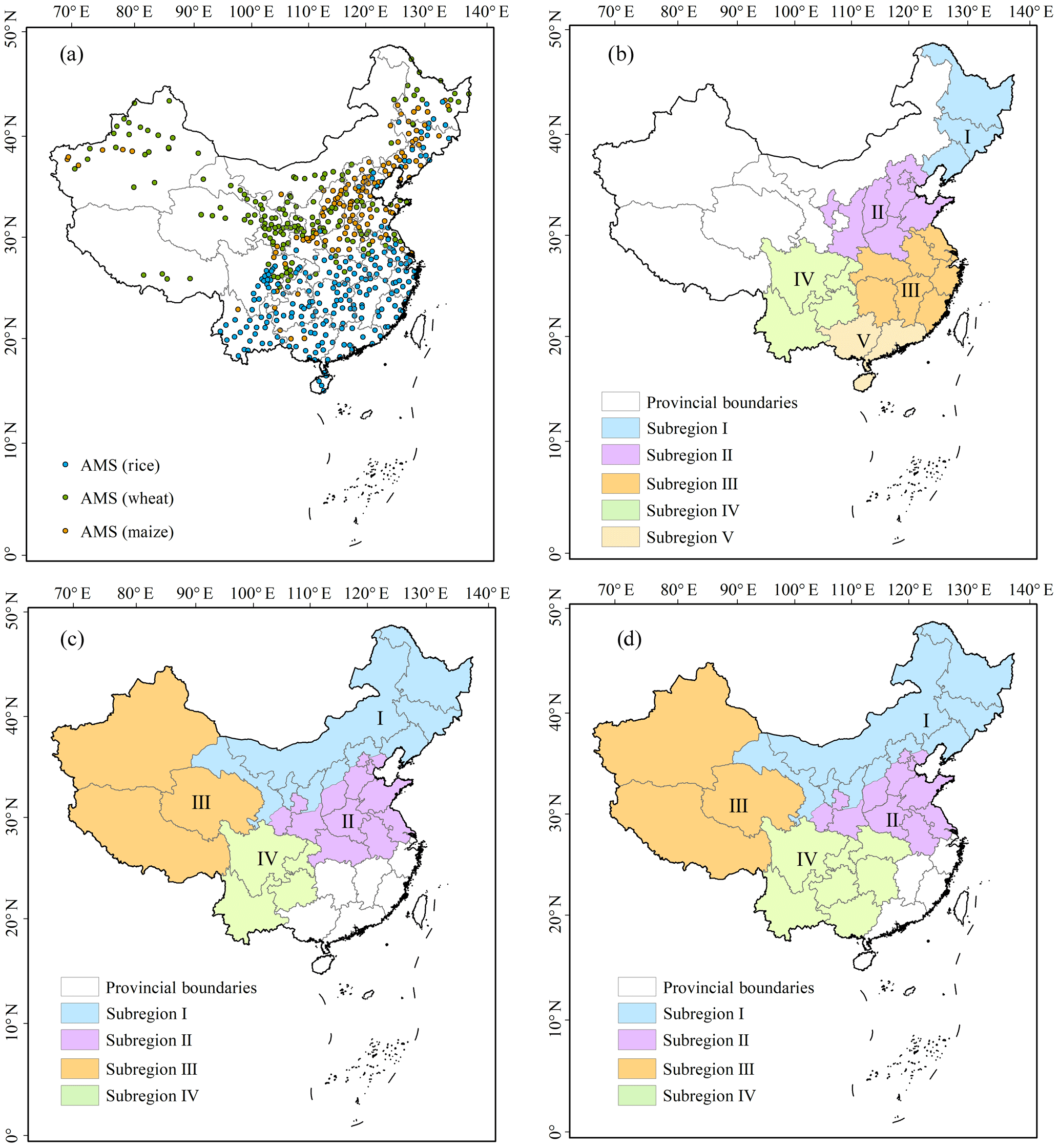
Figure 1The spatial distribution of agricultural meteorological stations (AMSs) in studied areas (a) and the locations of divided subregions for rice (b), wheat (c) and maize (d).
2.2 Data
2.2.1 ChinaCropPhen1km input data
An improved MODIS-based LAI dataset (GLASS LAI) from 2000 to 2015 was from Liang et al. (2013; http://glass-product.bnu.edu.cn/?pid=3&c=1, last access: January 2020). The GLASS LAI product was generated with general regression neural networks (GRNNs) trained by the fused LAI from MODIS and Carbon cYcle and Change in Land Observational Products from Ensemble of Satellites (CYCLOPES) LAI products and the reprocessed MODIS reflectance of the Benchmark Land Multisite Analysis and Intercomparison of Products (BELMANIP) sites during the period 2001–2003 (Liang et al., 2013). By computing the root-mean-square error (RMSE) and determination coefficients (R2) between several global LAI products and the high-resolution LAI reference map, it could be shown that the accuracy of the GLASS LAI (RMSE=0.78; R2=0.81) was fairly good compared to that of the MODIS LAI product (MOD15) and Geoland2 BioPar version 1 (GEOV1; Xiao et al., 2016). Moreover, the intercomparison indicated that the GLASS LAI (8 d composites of 1 km spatial resolution) was more temporally continuous and spatially complete than the other LAI products (Xiao et al., 2014, 2016). It has been applied to vegetation monitoring and crop model assimilation (Xiao et al., 2014; Chen et al., 2018a).
In addition, the cultivated-land layer derived from the 1 km National Land Cover Dataset (NLCD) of China was used as cropland masks. Specifically, we detected the key phenological dates for dryland crops (i.e., maize and wheat) and paddy rice, which were restricted on the dryland and paddy field layer derived from the NLCD, respectively. NLCD was provided by the Data Center for Resources and Environmental Sciences, Chinese Academy of Sciences (http://www.resdc.cn/Default.aspx, last access: January 2020), which also included several epochs of land use datasets, i.e., 2000, 2005, 2010 and 2015 (Liu et al., 2005, 2014).
2.2.2 ChinaCropPhen1km validation data
The crop phenology observation records from 2000 to 2013 of maize, rice and wheat crops were obtained from AMSs, which were governed by the CMA (https://data.cma.cn/, last access: December 2019). Such phenology information was observed and recorded by well-trained agricultural technicians in the experimental field and then checked and managed by the Chinese Agricultural Meteorological Monitoring System (CAMMS). In this study, we selected the agrometeorological stations with more than 10 years of records of key phenological dates, including the green-up date, emergence date, transplanting date, V3 stage (i.e., early vegetative stage of maize when the third leaf is fully expanded), heading date and maturity date, for the three crops. Totally, there were 436 stations across the main crop-cultivated areas in China (Fig. 1).
2.3 Methods
The method to retrieve the phenological information of three staple crops at the national scale is presented schematically in Fig. 2. The data processes are as follows: (1) data preprocessing, (2) selecting the cropland sample grid to determine the suitable smoothing method, (3) determining the optimal filter-based phenology detection (OFP) approach and (4) generating the ChinaCropPhen1km dataset.
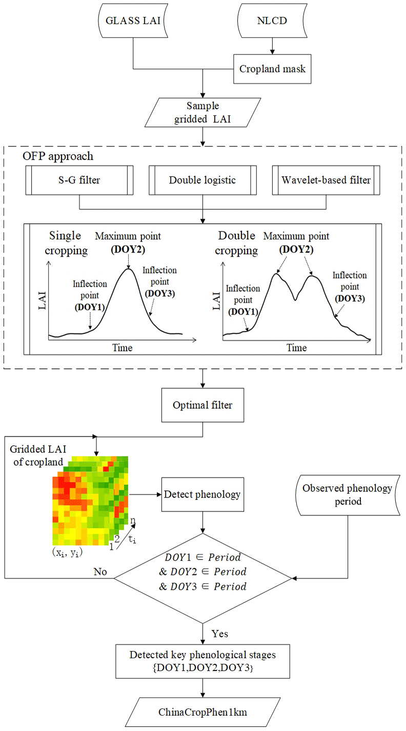
Figure 2Flow chart of procedures for data analysis and crop phenological date identification.
2.3.1 Data preprocessing
Due to the differences among these datasets on the projected coordinate system, firstly, we projected or re-projected all raster data to “Asia North Albers Equal Area Conic” by using the Project Raster tool in ArcGIS. Then, we combined 46 annual GLASS LAI images together and used a China provincial administrative vector map to mask images by province. Finally, a LAI time series was created for each pixel for further applications.
2.3.2 ChinaCropPhen1km LAI smoothing methods
Previous studies have proposed different smoothing methods to reduce the noise of GLASS LAI time series and found that the OFP method varied by studied times, areas and objectives (Zhao et al., 2016; Wang et al., 2018). Three commonly used methods were chosen in the study to smooth the LAI time-series curves, including the double logistic (DL) method, Savitzky–Golay (S-G) filter method and wavelet-based filter (WF) method.
Double logistic (DL) method
The double logistic method is a method of merging local fitting parts to obtain the overall fitting result (Jonsson and Eklundh, 2004). In the local fitting process, the double logistic function can be expressed as
where x1 determines the position of the left inflection point, while x2 gives the rate of change. Similarly, x3 determines the position of the right inflection point, while x4 gives the rate of change at this point.
Savitzky–Golay (S–G) filter method
Based on locally adaptive moving window, the S–G filtering method can be used to smooth data and suppress disturbances with a local polynomial regression model (Savitzky and Golay, 1964). The algorithm can be summarized as follows:
where LAIj+i represents the original LAI value, is the smoothed LAI value, j is running index of the LAI time series, Ci is the coefficient of the ith LAI value, n is the half-width of the smoothing window and N is the width of the moving window to perform filtering (2n+1). The width of the moving window – N – not only determines the degree of smoothing but also affects the ability to follow a rapid change. We selected three window widths (3, 4 and 5) to identify a better width for different crops and regions.
Wavelet-based filter (WF) method
The wavelet-based filter method can reduce noise with reflecting the periodicity of seasonal vegetation change (Sakamoto et al., 2005). The input signals f(x) is transformed in the wavelet transform as follows:
where a is a scaling parameter, b is a shifting parameter and φ implies a mother wavelet.
The advantage of the WF method is that it can maintain the time components of time-series data and hardly distort signals. The input signal f(x) is decomposed into linear combinations of wavelet functions in the multi-resolution approximation:
where f(x)i implies the approximate expression in level i, and g(x)i implies the high-frequency components in level i. We used three types of mother wavelets: Daubechies (1988; on the order of 3–24), Coiflet (on the order of 1–5) and Symlet (on the order of 4–15) in the study.
2.3.3 Methods to detect the phenological information
The methods to detect remote-sensing-based phenology can generally be classified into three groups: the inflection-based method (Chen et al., 2016), threshold-based method (Manfron et al., 2017), and methods based on the mathematical or geometrical model-fitting approach (Sakamoto et al., 2010). In this study, we used both the inflection- and threshold-based methods together to detect phenology. Firstly, we defined the inflection and maximum points of LAI time series as the specific timing of key phenological stages for different crops (Fig. 3).
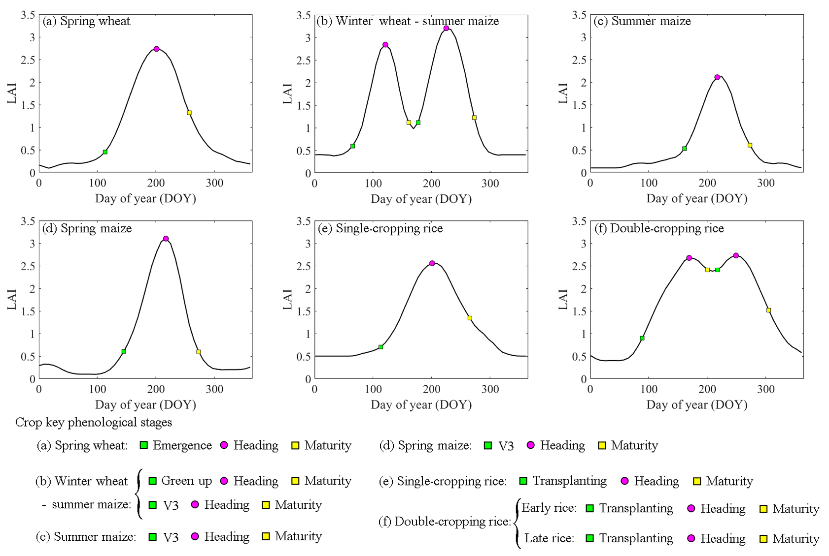
Green-up date, emergence date, transplanting date and V3 stage
We defined the date of inflection point (the first derivative increases continuously after this point or the second derivative equals 0) of the LAI time-series curves as the green-up date of winter wheat, emergence date of spring wheat, transplanting date of rice and V3 stage (early vegetative stage of maize when the third leaf is fully expanded) of maize (Sakamoto, 2018; Sakamoto et al., 2005, 2010). Before the inflection point, the LAI values are kept low for a long time, and then they start to increase continuously after this point.
Heading date
The heading date in the study was defined as the day when the LAI reaches the maximum, similar to some previous studies (Sakamoto et al., 2005; Chen et al., 2018b) – that is to say, the maximum LAI points in the time-series curve are regarded as the heading dates.
Maturity date
When crops reach maturity, the physiological activity will change largely, leading to an abrupt decrease in LAI (Sakamoto et al., 2005; Chen et al., 2018b). Therefore, we regarded an inflection point in the LAI time-series curve, where the first derivative is negative with the largest absolute value, as the maturity date.
2.3.4 Determining the optimal filter-based phenology detection approach (OFP)
Based on the observations around the nearest AMS, we needed firstly to determine the restricted time windows responding to each key phenological stage for different crops. Then we randomly sampled 1000 grids every year in each province from the grids where the land use data were identified as cropland and retrieved the key phenological stages in the sampling grids according to the three smoothing methods and the above definitions of key stages. To determine the OFP approach in each province, we identified the inflection points and maximum value point of each LAI time-series curve at each grid within the restricted time windows. After detecting phenological information of the cropland sample grids, we calculated the RMSE values between the estimated phenological dates and observed dates and averaged those RMSE values for each crop at a provincial scale. Finally, we chose the most suitable smoothing method for different crops in each province with minimum RMSE.
2.3.5 Generating ChinaCropPhen1km dataset
After removing the grids from where the land use data were identified as non-cropland, we then obtained cropland grids where the phenological information is detected. Then, the most suitable smoothing method for different crops in each province were applied to reconstruct the LAI time series at the 1 km grid scale. Finally, we detected the key phenological dates using the OFP approach and determined the cultivated grids for each crop on the basis of three key phenological stages that could be identified simultaneously. For example, if the green-up date, heading date and maturity date (corresponding to the inflection and maximum points in LAI time series) of winter wheat could be simultaneously detected for a specific grid, then it could be regarded as the cultivated grid of winter wheat. Additionally, to evaluate the accuracy of the estimated phenological dates at a national scale, we calculated the mean of phenological dates detected from each crop pixel around the corresponding AMS and compared them with the corresponding observations by using the RMSE.
3.1 Comparisons of different smoothing methods
The smoothed time profiles of the LAI generated by different smoothing methods are shown in Fig. 4. Both the S–G filter and WF method can smooth LAI time series well – that is to say, the generated time profiles of the LAI match well with the seasonal tendency of the observed LAI time series in the field. In addition, both methods can clearly characterize the local changes in the time component and maintain the time components of LAI time-series data. Although the DL method performs poorly for smoothing LAI time series of the double-season crops, it is still reliable for single-season crops. These findings were consistent with those in some previous studies (Zhu et al., 2012; Sakamoto et al., 2005; Qiu et al., 2016).
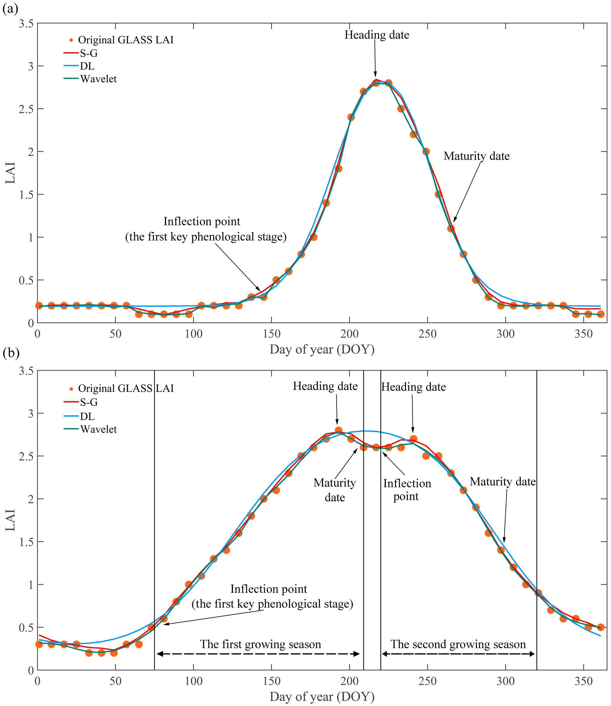
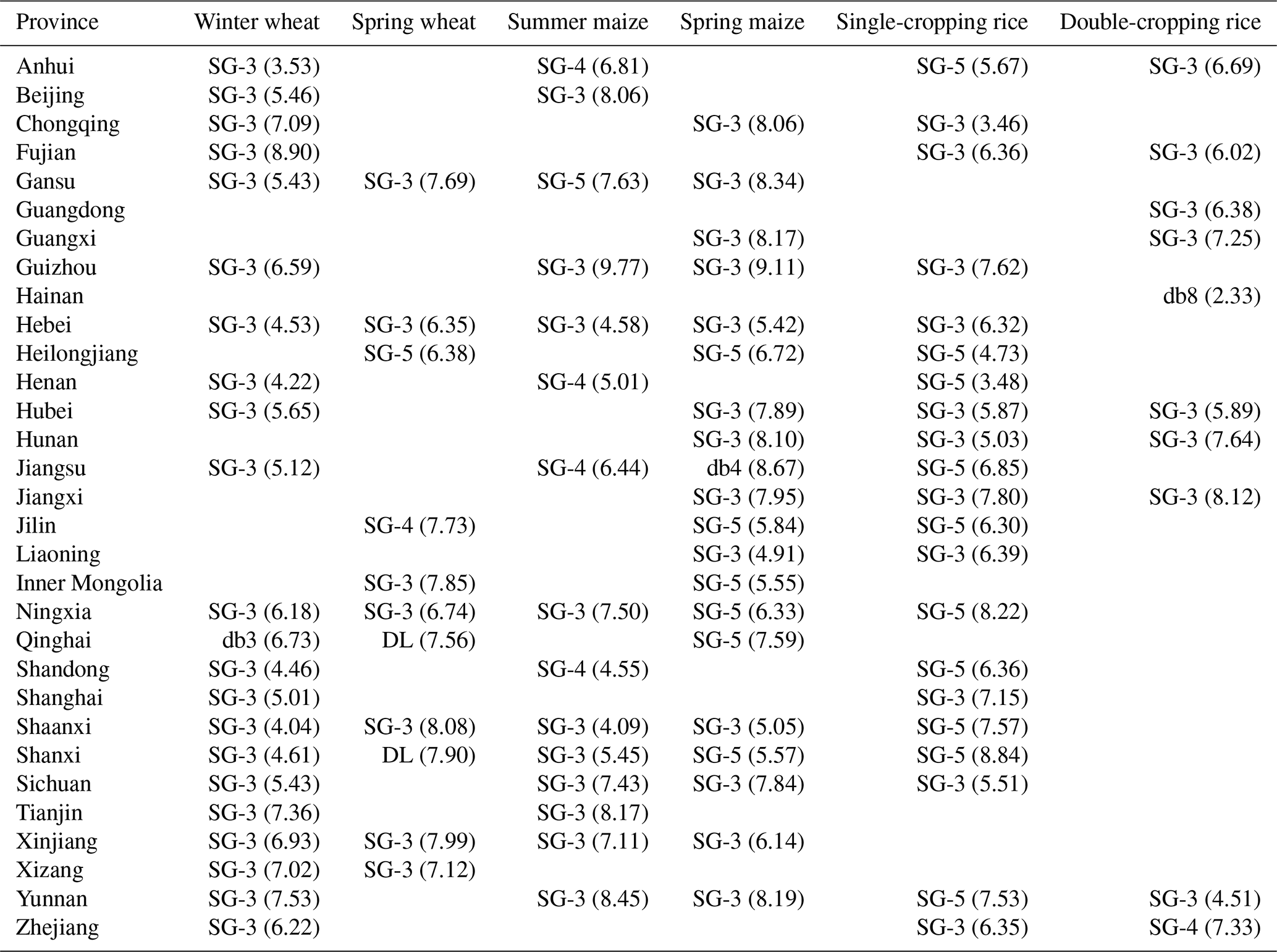
We further compared mean RMSE of different smoothing methods and selected the most suitable smoothing method with minimal mean RMSE for different provinces and crops (Table 1). If the RMSE values were the same, we also compared the number of crop grids according to different smoothing methods and selected the suitable method which had identified a larger number of crop girds. It is noted that the number of identified grids differ considerably even with same RMSE values. Totally, the S–G filter was an overwhelming smoothing method for 95 % crops and provinces, followed by the WF and DL method.
Table 1Mean RMSE (in parenthesis) of the most suitable smoothing method for different regions and crops.
We ascribed the great performance of the S–G to two reasons. (1) Its scientific smoothing principle is as follows: the S–G filter applies an iterative weighted moving average filter to the time series, which can replace the noise data as well as keep the fidelity (Geng et al., 2014). By contrast, the WF method decomposes the time series into scaled and shifted wavelets to acquire time localization of a given signal (Qiu et al., 2014). The DL method uses a series of parameters to fit the time series (Beck et al., 2006). (2) S–G is more suitable for the GLASS LAI. S–G can catch the local variations – e.g., the bimodal curve characteristics from double-cropping rice and the rotation of winter wheat and summer maize (Fig. 3b, f) – in time series and perform the best for data without extreme noise, such as those of the GLASS LAI (Eklundh and Jönsson, 2015). The DL method is more useful for data with much noise; however, it fails to identify local changes due to being unfit for data with double peaks. The WF method is also a powerful tool for processing non-stationary and noisy signals such as VI time series rather than the GLASS LAI (Rouyer et al., 2008; Sakamoto et al., 2006). Therefore, S–G is the most suitable for the complex cultivating systems across all of mainland China. We also attributed the excellent performance of S–G to the phenological extraction rules established in this paper and the goal of accurately extracting the crop cultivation grids as well as key phenology stages. For example, the WF smoothing method might eliminate pseudo-inflection points that may not be pseudo due to the uncertainty of GLASS LAI data and misidentify non-crop grids by inflection- and threshold-based methods, consequently resulting in very few crop grids being identified (Qiu et al., 2016).
3.2 Validation of ChinaCropPhen1km
The comparison between retrieved phenological dates and phenological observations of each crop from 2000–2015 at the national scale showed that all retrieved and observed dates were closely and averagely distributed on the 1:1 line for three crops (Fig. 5). Additionally, the RMSE values of retrieved phenological dates were consistently less than 10 d (Table 2). The RMSE averages of three key dates for rice were around 5.3 d, followed by wheat (5.5 d) and maize (6.7 d), corresponding to the related R2 of 0.98, 0.97 and 0.97, respectively.
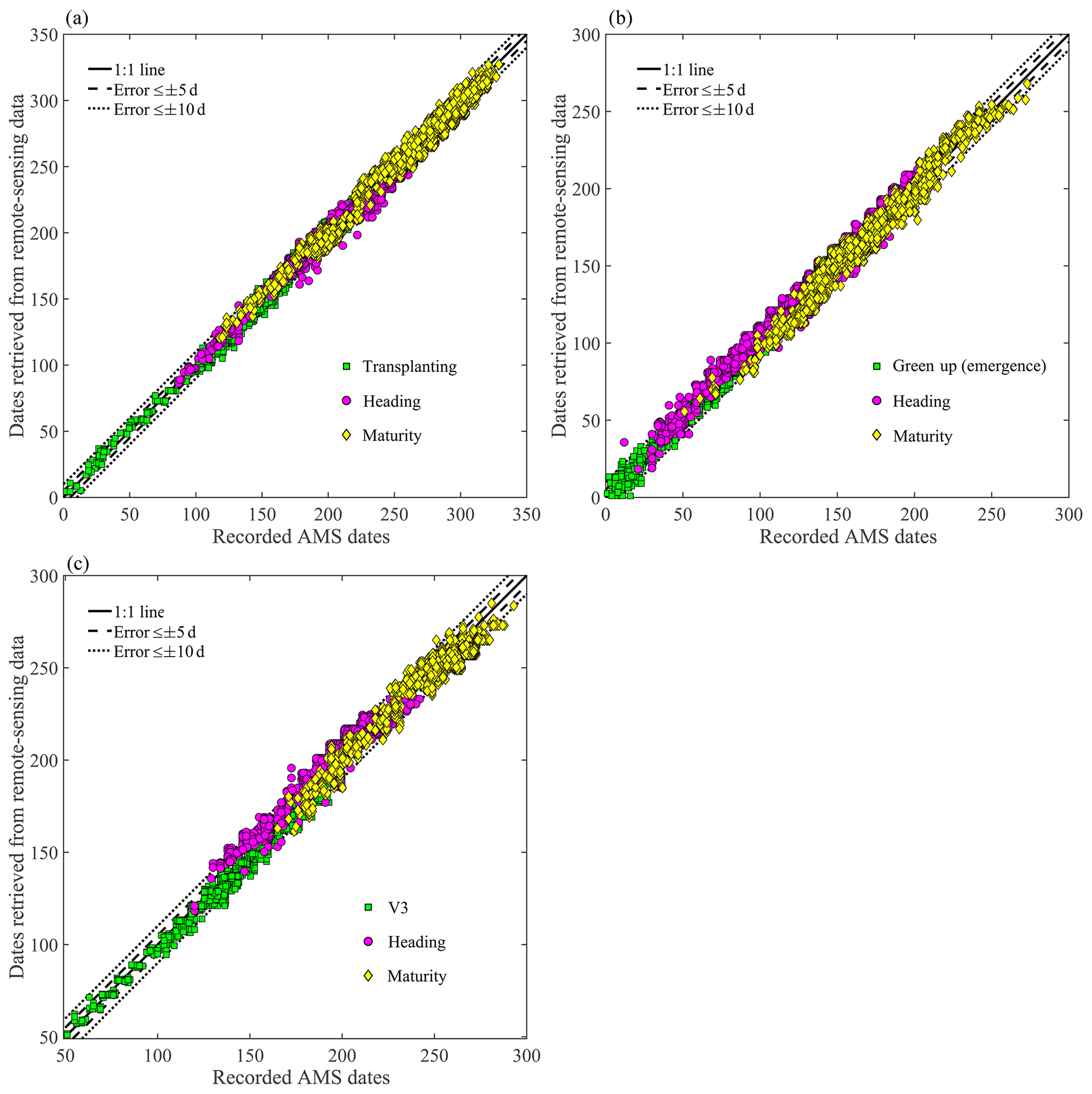
Figure 5Comparisons between retrieved and observed phenological dates for rice (a), wheat (b) and maize (c).
Table 2Mean RMSE between retrieved phenological dates and phenological observations.

As for the differences among crops, the retrieved accuracy of maize phenological stages was consistently the worst, with the biggest RMSE and errors ( d) and the lowest errors ( d) and R2. We ascribed the lower accuracy of maize phenology to the wider spatial heterogeneity environment and the complex-rotation planting system relative to the other two crops (Qiu et al., 2018). The highest accuracy of rice phenology also supported the accuracy impact of the complex planting system because the paddy field is unfit for dryland crops such as maize, wheat, soybean and other coarse cereals (Dong et al., 2015).
More interestingly, the retrieved accuracy of three crops decreased as crops grew and developed up to maturity periods (Table 2), with the average RMSEs ranging from 3.7 to 7.2 d. The highest accuracy (RMSE = 2.8; error = 0.5 %) was found for the green-up and emergence stages of wheat, while accuracy of the maturity stage for each crop was the lowest (average RMSE = 7.2; error = 19 %). The reasonable explanation might be relative weaker interference from other vegetation because the green-up and emergence stage occurs most early during the plant-growing period (some 80 DOY; Table 3). With the land surface green up, more and more information on plant-growing statuses will be found by satellites, which consequently mix with the crops' information and interfere with accurately retrieving the phenological stages of crops. Of course, the interference from anthropological activities should not be ignored with climate warming.
Table 3Annual mean phenological dates and growth periods of different crops in each subregion.
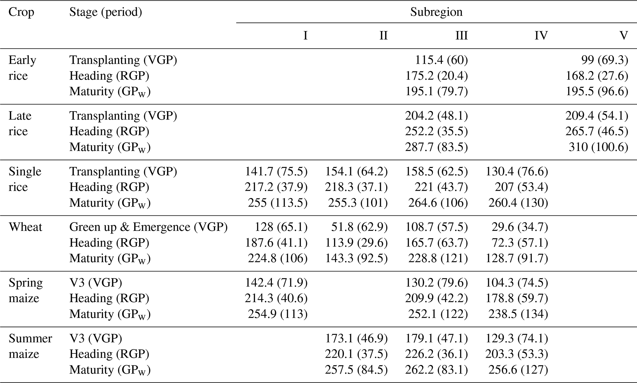
VGP means vegetative growth period – the difference between heading and transplanting or green-up or emergence or V3 dates. RGP means the reproductive growth period – the difference between maturity and heading dates. GPw means the whole growth period – the difference between maturity and transplanting or green-up or emergence or V3 dates. The numbers in the parentheses mean the annual mean growth periods.
Nevertheless, overall the retrieved phenological dates for the three crops are in strong correspondence with the observational dates (R2>0.95), and their relationships are statistically significant (p<0.01). Meanwhile, the growing status of other plants (or rotation crops, e.g., wheat—maize and maize–soybean) and the influence of other noises will lead to deviations of the remote-sensing LAI curve and the actual observed curve in the field. The noises also include other factors, e.g., weather conditions, farmers' behaviors, etc. However, the uncertainty does not exclude the applicability of our method to retrieve key phenological stages of crops, especially retrieving relative higher-resolution phenological information based on mature remote-sensing products at a large spatial scale.
3.3 Spatiotemporal patterns of key phenological stages from 2000 to 2015
We showed the annual averages of each key crop growth stage to indicate their spatiotemporal patterns due to the similarity in inter-annual patterns for a certain crop over the 16 years (Figs. 6–7, Table 3 and Supplement Figs. S1–S4). Besides summarizing the key stages by crops and subregions, we also calculated three crop growth periods, including the VGP (vegetative growth period), RGP (reproductive growth period) and GPW (whole growth period) to interpret their patterns (Fig. 8; Table 3). Among the five subregions with rice cultivation, subregion III was the most complex because three types of rice were cultivated there (Fig. 6a; Fig. 7a). The single-cropping rice in the subregion III was generally cultivated in the northern parts of four provinces (i.e., Anhui, Jiangsu, Zhejiang and Hubei), which was characterized by three key stages occurring later (DOY 159–265) than other three single-rice subregions (I, II and IV). Moving from the south (IV) to north (I) (excluding subregion III because of cultivation of double-cropping rice), single-cropping rice was not transplanted in sequence as expected. In subregion II, it was transplanted latest (DOY 154) but had relatively early maturity dates (DOY 255), resulting in the shortest growing period (101 d; Fig. 8a). On the contrary, in subregion IV, single-cropping rice was transplanted earliest but had the maturity occurring latest, resulting in the longest growing period of 130 d (Figs. 6a, 7a, 8a). In subregion V, where only double-cropping rice was cultivated, early-season rice was transplanted earlier (DOY 99) and maturity dates of late-season rice occurred later (DOY 310), consequently resulting in longer growing periods (97 and 101 d for corresponding early-season and late-season rice) than those in subregion III with double-rice cultivation (80 and 84 d; Table 3).
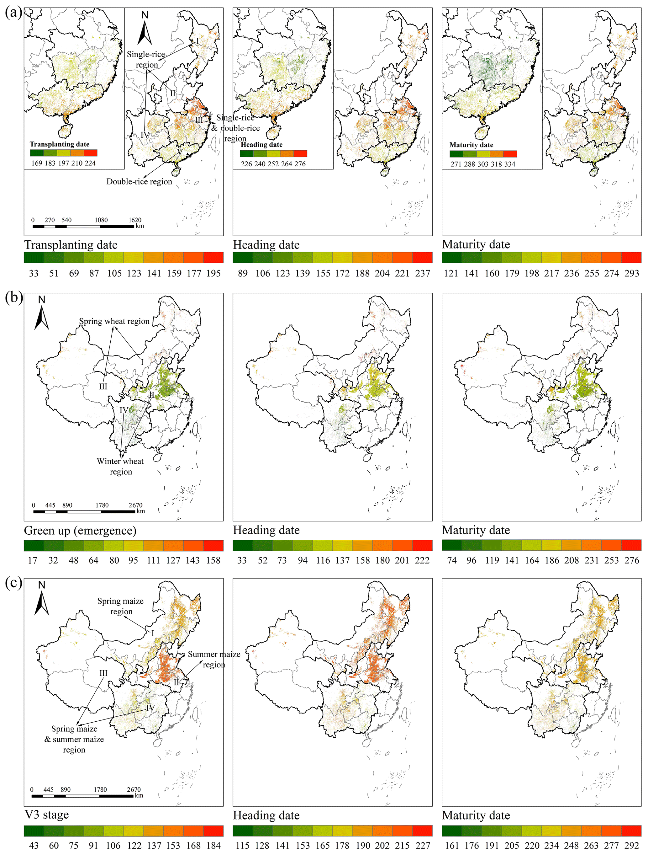
Figure 6Spatial patterns of annual averages of three key phenological dates during 2000–2015 for rice (a), wheat (b) and maize (c).

Figure 7Box plots of three key phenological dates by crop and subregions during 2000–2015 for rice (a), wheat (b) and maize (c).
As for wheat, green-up and emergence dates ranged most widely (DOY 30–128) when compared to other crops. Winter wheat in subregions II and IV had earlier green-up dates, while spring wheat in subregions I and III had later emergence dates (Table 3; Figs. 6b, 7b). Moreover, along with the latitudes from the north to the south (excluding subregion III because of the sparsest wheat cultivation being there), the first key dates were earlier, but with shorter growth periods (106, 93 and 92 d for I, II and IV) due to the sufficient temperature and light in subregion IV (Yu et al., 2012; Fig. 8b). Interestingly, the heading and maturity dates in the three subregions showed consistently the same spatial patterns as those of the first stage, with latitudes decreasing (Figs. 6b, 7b).

Figure 8Box plots of three key phenological periods by crop and subregions during 2000–2015, for vegetative growth period (VGP); reproductive growth period (VGP); and whole growth period (GPW) of rice (a), wheat (b) and maize (c).
Both spring and summer maize types were concurrently cultivated in subregions III and IV, while only one of them was cultivated in subregions I and II, the main planting areas of northern China (Figs. 6c, 7c; Table 3). V3 of summer maize was approximately 43 d later than that of spring maize (DOY 161 vs. 117), but its maturity dates were very close (DOY 259 vs. 245), which thus caused a shorter growth period for summer maize, especially for subregions II and III (some 84 d; Fig. 8c). Additionally, in three subregions (I, III and IV) for spring maize, like wheat, the spatial patterns of the three key stages for maize were similar in spatial patterns with increasing latitude. Finally, the key dates and periods were the most variable in subregion IV (Figs. 7c, 8c).
In sum, the spatial patterns of key phenological stages varied by crops and cultivation methods. In addition, early-season rice and single-cropping rice in subregion III, wheat in subregion III, and maize and rice in subregion IV showed larger variability than other crops due to the mixed planting of heterogeneous varieties of the same crop. Many factors could impact crop phenology, such as climate, environment, farmer's behaviors, technological development and human activities (Liu et al., 2016, 2018). Different from natural ecosystems such as wild forest or grassland, three main crops cultivated across the mainland of China did not reach green-up or flowering dates in sequence with latitude, especially for rice (Zhang et al., 2014b, 2015; Tao et al., 2014). Moreover, climate conditions did impact crop phenology. For example, increased temperature led to the advanced heading and maturity date of crops in China (He et al., 2015; Tao et al., 2014). At the same time, crop management activities, such as cultivar shift and the adjustment of the planting and harvesting date, largely affected crop phenology (Tao et al., 2006, 2013).
3.4 The changes in three key phenological dates and growth periods from 2000 to 2015
To interpret the changes of the three key phenological dates and growth periods from 2000 to 2015, we analyzed their trends at the pixel scale and summarized the grids with a significant trend (p<0.1) according to crops and subregions (Figs. 9–10; Table 4). We found more positive trends, with 0.78 d yr−1 for 70 % summarized medians, but fewer negative ones, with −0.69 d yr−1 and 30 % medians. This suggests that phenological dates were delayed. Specifically, the proportion of pixels that had a positive trend is 92 % for wheat (Fig. 9b), 75 % for rice (Fig. 9a) and 50 % for maize (Fig. 9c).
Table 4The trend (d yr−1) of three key phenological dates and growth periods from 2000 to 2015.
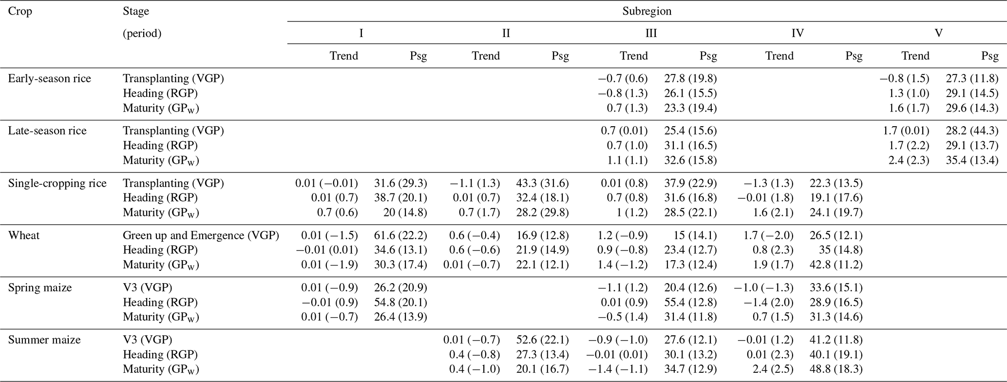
Note: definitions for the VGP, RGP and GPw as in Table 3. Psg (%) means the percent of grids showing significant trend at the p<0.1 level. The numbers in the parentheses mean the statistic values of grids during three growth periods.

Figure 9The trends of three key phenological dates during 2000–2015 by crop and subregions for rice (a), wheat (b) and maize (c).

Figure 10The trends of three key phenological periods during 2000–2015 by crop and subregions. VGP stands for vegetative growth period; RGP for reproductive growth period; and GPW for whole growth period of rice (a), wheat (b) and maize (c).
For rice, transplanting dates were consistently advanced by −0.64 d yr−1 for early-season rice and single-cropping rice and delayed by 0.84 d yr−1 for late-season rice in most areas. Maturity dates became later by 1.23 d yr−1, but heading dates had fewer changes. In addition, double-cropping rice in subregion III showed less variability than that in subregion V (Fig. 9a). By contrast, the first stages (i.e., green-up and emergence stage) were delayed by 0.88 d yr−1 consistently for almost all of the wheat cultivation areas (Fig. 9b). Maize in the subregion II, and wheat in subregion I and II (Fig. 9b), had an opposite trend to that of rice (Fig. 9; Table 4). Moreover, the changes in the three stages showed less variable in subregion II, the main planting areas for both dryland crops. Among all the crops and growth stages, maize in the regions III and IV had consistently negative trends, with the exception of maturity dates in subregion IV.
Compared with the significant changes in phenological dates, the duration of phenological periods changed with fewer pixels (<30 %; Table 4). More pixels with positive trends, with 1.25 d yr−1 for 66.7 % medians, were identified than those with negative trends, with −0.97 d yr−1 for 32.3 % medians, implying commonly prolonged growth periods during the study period; 95.8 % of the medians were positive for rice, while 75 % of the medians were negative for wheat. The changes of maize growth periods were similar to those of their phenological dates.
The duration of growth periods was prolonged, especially for the whole growth period (GPw), which was consistently observed for rice cropping systems, except for early-season rice in subregion V. In addition, the duration of the VGP for single-cropping rice in subregion I had weaker trends (Fig. 10a). On the contrary, almost all the wheat growth periods were shortened, except for winter wheat in subregion V, especially for spring wheat in the subregion I (Fig. 10b). Additionally, in terms of growth period duration, maize had similar changes to wheat in subregions I and II. Changes in growth period duration were different for spring (shortened) and winter (prolonged) wheat and for both maize types between subregion III and IV (Fig. 10c). The results are well supported by some previous studies based on the intensive observations at the site scale (Tao et al., 2012, 2013, 2014; Zhang et al., 2014b).
3.5 Uncertainties in ChinaCropPhen1km
Inevitably, there are still uncertainty in the generated dataset (i.e., ChinaCropPhen1km). On the one hand, GLASS LAI products might lead to some uncertainty in ChinaCropPhen1km. First of all, the noise of the original GLASS LAI time series could reduce the accuracy of detected phenological stages, which resulted from many factors, such as cloud, snow, aerosols and water vapor (Xiao et al., 2014). Therefore, we compared several commonly used smoothing methods and chose the most suitable one with minimum RMSE for different crops in each province, which could reduce some uncertainty. Moreover, the GLASS LAI retrieval algorithm eliminates abrupt spikes and dips, which may result in the loss of neighboring smaller peaks in LAI profiles (Xiao et al., 2016). The number of detected pixels with the double-season rice cultivated might be less than that of the actual situation due to the short interval between the two local maximum points (i.e., heading stages of early-season rice and late-season rice; Fig. 3f). On the other hand, the mixed pixel might bring uncertainty in the results, as it contained several land cover types and then weakened the identified signal of specific phenological stages. We ascribed the occurrence of mixed pixel to two reasons. One is the coarse spatial resolution of 1 km. For example, the mixed pixel occurs widely in the mountainous regions (e.g., southern China) with complex terrain and diverse vegetation types. The other is that we determined the spatial distribution of each dryland crop (i.e., maize and wheat) based on the dryland layer of NLCD, which might include several crop types. In future studies, the application of a crop-specific map and remote-sensing products with finer spatial resolution is expected to solve the mixed pixel issues.
The derived crop phenological dataset for three staple crops in China during 2000–2015 is available at https://doi.org/10.6084/m9.figshare.8313530 (Luo et al., 2019).
In the present study, we generated a 1 km gridded-phenology dataset for three main crops from 2000 to 2015 based on GLASS LAI products, called ChinaCropPhen1km. First, we compared three common smoothing methods and chose the most suitable one for different crops and regions. The results showed that S–G was the most frequently chosen method, as it could not only smooth the time series well but also keep the fidelity. Next, we developed an OFP approach which combined both the inflection- and threshold-based method to detect the key phenological stages of three staple crops at a spatial resolution of 1 km across China. Finally, we established a high-resolution gridded-phenology product for three staple crops in China during 2000–2015.
The ChinaCropPhen1km dataset was validated well using the intensive phenological observations of AMS, which substantiates high accuracy, with errors of retrieved phenological date of less than 10 d. It can reflect the spatial differences in the local climatic and management factors. Thus, this first high-resolution crop phenological dataset can be applied for many purposes, including understanding land surface phenological dynamics, investigating climate change impacts and adaptations, and improving agricultural-system or earth-system modeling over a large area, temporally and spatially.
The supplement related to this article is available online at: https://doi.org/10.5194/essd-12-197-2020-supplement.
ZZ and YC designed the research. YC and ZL collected datasets. YL implemented the research and wrote the paper. ZZ and FT revised the paper.
The authors declare that they have no conflict of interest.
We would like to thank the high-performance computing support from the Center for Geodata and Analysis, Faculty of Geographical Science, Beijing Normal University (https://gda.bnu.edu.cn/, last access: January 2020).
This research has been supported by the National Key Research and Development Program of China (project nos. 2019YFA0607401 and 2017YFD0300301) and the National Basic Research Program of China (grant nos. 41977405, 31561143003, 31761143006).
This paper was edited by Birgit Heim and reviewed by two anonymous referees.
Atzberger, C., Klisch, A., Mattiuzzi, M., and Vuolo, F.: Phenological Metrics Derived over the European Continent from NDVI3g Data and MODIS Time Series, Remote Sens.-Basel, 6, 257–284, https://doi.org/10.3390/rs6010257, 2014.
Beck, P. S. A., Atzberger, C., Hogda, K. A., Johansen, B., and Skidmore, A. K.: Improved monitoring of vegetation dynamics at very high latitudes: A new method using MODIS NDVI, Remote Sens. Environ., 100, 321–334, https://doi.org/10.1016/j.rse.2005.10.021, 2006.
Bolten, J. D., Crow, W. T., Zhan, X. W., Jackson, T. J., and Reynolds, C. A.: Evaluating the Utility of Remotely Sensed Soil Moisture Retrievals for Operational Agricultural Drought Monitoring, IEEE J.-Stars, 3, 57–66, https://doi.org/10.1109/Jstars.2009.2037163, 2010.
Bolton, D. K. and Friedl, M. A.: Forecasting crop yield using remotely sensed vegetation indices and crop phenology metrics, Agr. Forest Meteorol., 173, 74–84, https://doi.org/10.1016/j.agrformet.2013.01.007, 2013.
Brown, M. E., de Beurs, K. M., and Marshall, M.: Global phenological response to climate change in crop areas using satellite remote sensing of vegetation, humidity and temperature over 26 years, Remote Sens. Environ., 126, 174–183, https://doi.org/10.1016/j.rse.2012.08.009, 2012.
Cao, R. Y., Chen, J., Shen, M. G., and Tang, Y. H.: An improved logistic method for detecting spring vegetation phenology in grasslands from MODIS EVI time-series data, Agr. Forest Meteorol., 200, 9–20, https://doi.org/10.1016/j.agrformet.2014.09.009, 2015.
Chen, Y., Zhang, Z., and Tao, F. L.: Improving regional winter wheat yield estimation through assimilation of phenology and leaf area index from remote sensing data, Eur. J. Agron., 101, 163–173, https://doi.org/10.1016/j.eja.2018.09.006, 2018a.
Chen, Y., Zhang, Z., Tao, F. L., Palosuo, T., and Rotter, R. P.: Impacts of heat stress on leaf area index and growth duration of winter wheat in the North China Plain, Field Crop. Res., 222, 230–237, https://doi.org/10.1016/j.fcr.2017.06.007, 2018b.
Chen, Y. L., Song, X. D., Wang, S. S., Huang, J. F., and Mansaray, L. R.: Impacts of spatial heterogeneity on crop area mapping in Canada using MODIS data, Isprs J. Photogramm., 119, 451–461, https://doi.org/10.1016/j.isprsjprs.2016.07.007, 2016.
Curnel, Y., de Wit, A. J. W., Duveiller, G., and Defourny, P.: Potential performances of remotely sensed LAI assimilation in WOFOST model based on an OSS Experiment, Agr. Forest Meteorol., 151, 1843–1855, https://doi.org/10.1016/j.agrformet.2011.08.002, 2011.
Daubechies, I.: Orthonormal Bases Of Compactly Supported Wavelets, Commun. Pur. Appl. Math., 41, 909–996, https://doi.org/10.1002/cpa.3160410705, 1988.
de Wit, A. M. and van Diepen, C. A.: Crop model data assimilation with the Ensemble Kalman filter for improving regional crop yield forecasts, Agr. Forest Meteorol., 146, 38–56, https://doi.org/10.1016/j.agrformet.2007.05.004, 2007.
Dong, J. W., Xiao, X. M., Kou, W. L., Qin, Y. W., Zhang, G. L., Li, L., Jin, C., Zhou, Y. T., Wang, J., Biradar, C., Liu, J. Y., and Moore, B.: Tracking the dynamics of paddy rice planting area in 1986–2010 through time series Landsat images and phenology-based algorithms, Remote Sens. Environ., 160, 99–113, https://doi.org/10.1016/j.rse.2015.01.004, 2015.
Dorigo, W. A., Zurita-Milla, R., de Wit, A. J. W., Brazile, J., Singh, R., and Schaepman, M. E.: A review on reflective remote sensing and data assimilation techniques for enhanced agroecosystem modeling, Int. J. Appl. Earth Obs., 9, 165–193, https://doi.org/10.1016/j.jag.2006.05.003, 2007.
Eklundh, L. and Jönsson, P.: TIMESAT: A Software Package for Time-Series Processing and Assessment of Vegetation Dynamics, 141–158, https://doi.org/10.1007/978-3-319-15967-6_7, 2015.
Frolking, S., Qiu, J. J., Boles, S., Xiao, X. M., Liu, J. Y., Zhuang, Y. H., Li, C. S., and Qin, X. G.: Combining remote sensing and ground census data to develop new maps of the distribution of rice agriculture in China, Global Biogeochem. Cy., 16, 1091, https://doi.org/10.1029/2001gb001425, 2002.
Geng, L. Y., Ma, M. G., Wang, X. F., Yu, W. P., Jia, S. Z., and Wang, H. B.: Comparison of Eight Techniques for Reconstructing Multi-Satellite Sensor Time-Series NDVI Data Sets in the Heihe River Basin, China, Remote Sens.-Basel, 6, 2024–2049, https://doi.org/10.3390/rs6032024, 2014.
He, L., Asseng, S., Zhao, G., Wu, D. R., Yang, X. Y., Zhuang, W., Jin, N., and Yu, Q.: Impacts of recent climate warming, cultivar changes, and crop management on winter wheat phenology across the Loess Plateau of China, Agr. Forest Meteorol., 200, 135–143, https://doi.org/10.1016/j.agrformet.2014.09.011, 2015.
Huang, J. X., Ma, H. Y., Su, W., Zhang, X. D., Huang, Y. B., Fan, J. L., and Wu, W. B.: Jointly Assimilating MODIS LAI and ET Products Into the SWAP Model for Winter Wheat Yield Estimation, IEEE J.-Stars, 8, 4060–4071, https://doi.org/10.1109/Jstars.2015.2403135, 2015.
Ines, A. V. M., Das, N. N., Hansen, J. W., and Njoku, E. G.: Assimilation of remotely sensed soil moisture and vegetation with a crop simulation model for maize yield prediction, Remote Sens. Environ., 138, 149–164, https://doi.org/10.1016/j.rse.2013.07.018, 2013.
Jin, X. L., Kumar, L., Li, Z. H., Feng, H. K., Xu, X. G., Yang, G. J., and Wang, J. H.: A review of data assimilation of remote sensing and crop models, Eur. J. Agron., 92, 141–152, https://doi.org/10.1016/j.eja.2017.11.002, 2018.
Jonsson, P. and Eklundh, L.: TIMESAT – a program for analyzing time-series of satellite sensor data, Comput. Geosci.-UK, 30, 833–845, https://doi.org/10.1016/j.cageo.2004.05.006, 2004.
Liang, S. L., Zhao, X., Liu, S. H., Yuan, W. P., Cheng, X., Xiao, Z. Q., Zhang, X. T., Liu, Q., Cheng, J., Tang, H. R., Qu, Y. H., Bo, Y. C., Qu, Y., Ren, H. Z., Yu, K., and Townshend, J.: A long-term Global LAnd Surface Satellite (GLASS) data-set for environmental studies, Int. J. Digit. Earth, 6, 5–33, https://doi.org/10.1080/17538947.2013.805262, 2013.
Liao, C. H., Wang, J. F., Dong, T. F., Shang, J. L., Liu, J. G., and Song, Y.: Using spatio-temporal fusion of Landsat-8 and MODIS data to derive phenology, biomass and yield estimates for corn and soybean, Sci. Total Environ., 650, 1707–1721, https://doi.org/10.1016/j.scitotenv.2018.09.308, 2019.
Liu, J. Y., Liu, M. L., Tian, H. Q., Zhuang, D. F., Zhang, Z. X., Zhang, W., Tang, X. M., and Deng, X. Z.: Spatial and temporal patterns of China's cropland during 1990–2000: An analysis based on Landsat TM data, Remote Sens. Environ., 98, 442–456, https://doi.org/10.1016/j.rse.2005.08.012, 2005.
Liu, J. Y., Kuang, W. H., Zhang, Z. X., Xu, X. L., Qin, Y. W., Ning, J., Zhou, W. C., Zhang, S. W., Li, R. D., Yan, C. Z., Wu, S. X., Shi, X. Z., Jiang, N., Yu, D. S., Pan, X. Z., and Chi, W. F.: Spatiotemporal characteristics, patterns, and causes of land-use changes in China since the late 1980s, J. Geogr. Sci., 24, 195–210, https://doi.org/10.1007/s11442-014-1082-6, 2014.
Liu, Q., Fu, Y. S. H., Zhu, Z. C., Liu, Y. W., Liu, Z., Huang, M. T., Janssens, I. A., and Piao, S. L.: Delayed autumn phenology in the Northern Hemisphere is related to change in both climate and spring phenology, Glob. Change Biol., 22, 3702–3711, https://doi.org/10.1111/gcb.13311, 2016.
Liu, Y. J., Chen, Q. M., Ge, Q. S., Dai, J. H., Qin, Y., Dai, L., Zou, X. T., and Chen, J.: Modelling the impacts of climate change and crop management on phenological trends of spring and winter wheat in China, Agr. Forest Meteorol., 248, 518–526, https://doi.org/10.1016/j.agrformet.2017.09.008, 2018.
Liu, Z. J., Wu, C. Y., Liu, Y. S., Wang, X. Y., Fang, B., Yuan, W. P., and Ge, Q. S.: Spring green-up date derived from GIMMS3g and SPOT-VGT NDVI of winter wheat cropland in the North China Plain, Isprs J. Photogramm., 130, 81–91, https://doi.org/10.1016/j.isprsjprs.2017.05.015, 2017.
Luo, Y., Zhang, Z., Chen, Y., Li, Z., and Tao, F.: ChinaCropPhen1km: A high-resolution crop phenological dataset for three staple crops in China during 2000–2015 based on LAI products, https://doi.org/10.6084/m9.figshare.8313530, 2019.
Manfron, G., Delmotte, S., Busetto, L., Hossard, L., Ranghetti, L., Brivio, P. A., and Boschetti, M.: Estimating inter-annual variability in winter wheat sowing dates from satellite time series in Camargue, France, Int. J. Appl. Earth Obs., 57, 190–201, https://doi.org/10.1016/j.jag.2017.01.001, 2017.
Nearing, G. S., Crow, W. T., Thorp, K. R., Moran, M. S., Reichle, R. H., and Gupta, H. V.: Assimilating remote sensing observations of leaf area index and soil moisture for wheat yield estimates: An observing system simulation experiment, Water Resour Res, 48, W05525, https://doi.org/10.1029/2011wr011420, 2012.
Pan, Z. K., Huang, J. F., Zhou, Q. B., Wang, L. M., Cheng, Y. X., Zhang, H. K., Blackburn, G. A., Yan, J., and Liu, J. H.: Mapping crop phenology using NDVI time-series derived from HJ-1 A/B data, Int. J. Appl. Earth Obs., 34, 188–197, https://doi.org/10.1016/j.jag.2014.08.011, 2015.
Piao, S. L., Ciais, P., Huang, Y., Shen, Z. H., Peng, S. S., Li, J. S., Zhou, L. P., Liu, H. Y., Ma, Y. C., Ding, Y. H., Friedlingstein, P., Liu, C. Z., Tan, K., Yu, Y. Q., Zhang, T. Y., and Fang, J. Y.: The impacts of climate change on water resources and agriculture in China, Nature, 467, 43–51, https://doi.org/10.1038/nature09364, 2010.
Qiu, B. W., Zhong, M., Tang, Z. H., and Wang, C. Y.: A new methodology to map double-cropping croplands based on continuous wavelet transform, Int. J. Appl. Earth Obs., 26, 97–104, https://doi.org/10.1016/j.jag.2013.05.016, 2014.
Qiu, B. W., Li, W. J., Tang, Z. H., Chen, C. C., and Qi, W.: Mapping paddy rice areas based on vegetation phenology and surface moisture conditions, Ecol. Indic., 56, 79–86, https://doi.org/10.1016/j.ecolind.2015.03.039, 2015.
Qiu, B. W., Feng, M., and Tang, Z. H.: A simple smoother based on continuous wavelet transform: Comparative evaluation based on the fidelity, smoothness and efficiency in phenological estimation, Int. J. Appl. Earth Obs., 47, 91–101, https://doi.org/10.1016/j.jag.2015.11.009, 2016.
Qiu, B. W., Huang, Y. Z., Chen, C. C., Tang, Z. H., and Zou, F. L.: Mapping spatiotemporal dynamics of maize in China from 2005 to 2017 through designing leaf moisture based indicator from Normalized Multi-band Drought Index, Comput. Electron. Agr., 153, 82–93, https://doi.org/10.1016/j.compag.2018.07.039, 2018.
Rouyer, T., Fromentin, J., Stenseth, N. C., Cazelles, B.: Analysing multiple time series and extending significance testing in wavelet analysis, Mar. Ecol.-Prog. Ser., 359, 11–23, https://doi.org/10.3354/meps07330, 2008.
Sakamoto, T., Nguyen, N. V., Ohno, H., Ishitsuka, N., and Yokozawa, M.: Spatio-temporal distribution of rice phenology and cropping systems in theMekong Delta with special reference to the seasonal water flow of the Mekong and Bassac rivers, Remote Sens. Environ., 100, 1–16, https://doi.org/10.1016/j.rse.2005.09.007, 2006.
Sakamoto, T.: Refined shape model fitting methods for detecting various types of phenological information on major US crops, Isprs J. Photogramm., 138, 176–192, https://doi.org/10.1016/j.isprsjprs.2018.02.011, 2018.
Sakamoto, T., Yokozawa, M., Toritani, H., Shibayama, M., Ishitsuka, N., and Ohno, H.: A crop phenology detection method using time-series MODIS data, Remote Sens. Environ., 96, 366–374, https://doi.org/10.1016/j.rse.2005.03.008, 2005.
Sakamoto, T., Wardlow, B. D., Gitelson, A. A., Verma, S. B., Suyker, A. E., and Arkebauer, T. J.: A Two-Step Filtering approach for detecting maize and soybean phenology with time-series MODIS data, Remote Sens. Environ., 114, 2146–2159, https://doi.org/10.1016/j.rse.2010.04.019, 2010.
Sakamoto, T., Gitelson, A. A., and Arkebauer, T. J.: MODIS-based corn grain yield estimation model incorporating crop phenology information, Remote Sens. Environ., 131, 215–231, https://doi.org/10.1016/j.rse.2012.12.017, 2013.
Savitzky, A. and Golay, M. J. E.: Smoothing + Differentiation Of Data by Simplified Least Squares Procedures, Anal. Chem., 36, 1627, https://doi.org/10.1021/ac60214a047, 1964.
Tao, F., Yokozawa, M., and Zhang, Z.: Modelling the impacts of weather and climate variability on crop productivity over a large area: A new process-based model development, optimization, and uncertainties analysis, Agr. Forest Meteorol., 149, 831–850, https://doi.org/10.1016/j.agrformet.2008.11.004, 2009.
Tao, F. L., Yokozawa, M., Xu, Y. L., Hayashi, Y., and Zhang, Z.: Climate changes and trends in phenology and yields of field crops in China, 1981–2000, Agr. Forest Meteorol., 138, 82–92, https://doi.org/10.1016/j.agrformet.2006.03.014, 2006.
Tao, F. L., Zhang, S. A., and Zhang, Z.: Spatiotemporal changes of wheat phenology in China under the effects of temperature, day length and cultivar thermal characteristics, Eur. J. Agron., 43, 201–212, https://doi.org/10.1016/j.eja.2012.07.005, 2012.
Tao, F. L., Zhang, Z., Shi, W. J., Liu, Y. J., Xiao, D. P., Zhang, S., Zhu, Z., Wang, M., and Liu, F. S.: Single rice growth period was prolonged by cultivars shifts, but yield was damaged by climate change during 1981–2009 in China, and late rice was just opposite, Glob. Change Biol., 19, 3200–3209, https://doi.org/10.1111/gcb.12250, 2013.
Tao, F. L., Zhang, S., Zhang, Z., and Rotter, R. P.: Maize growing duration was prolonged across China in the past three decades under the combined effects of temperature, agronomic management, and cultivar shift, Glob. Change Biol., 20, 3686–3699, https://doi.org/10.1111/gcb.12684, 2014.
Tao, J. B., Wu, W. B., Zhou, Y., Wang, Y., and Jiang, Y.: Mapping winter wheat using phenological feature of peak before winter on the North China Plain based on time-series MODIS data, J. Integr. Agr., 16, 348–359, https://doi.org/10.1016/S2095-3119(15)61304-1, 2017.
Verger, A., Filella, I., Baret, F., and Penuelas, J.: Vegetation baseline phenology from kilometric global LAI satellite products, Remote Sens. Environ., 178, 1–14, https://doi.org/10.1016/j.rse.2016.02.057, 2016.
Wang, C. Z., Zhang, Z., Chen, Y., Tao, F. L., Zhang, J., and Zhang, W.: Comparing different smoothing methods to detect double-cropping rice phenology based on LAI products - a case study in the Hunan province of China, Int. J. Remote Sens., 39, 6405–6428, https://doi.org/10.1080/01431161.2018.1460504, 2018.
Wang, H. S., Chen, J. S., Wu, Z. F., and Lin, H.: Rice heading date retrieval based on multi-temporal MODIS data and polynomial fitting, Int. J. Remote Sens., 33, 1905–1916, https://doi.org/10.1080/01431161.2011.603378, 2012.
Wang, N., Wang, J., Wang, E. L., Yu, Q., Shi, Y., and He, D.: Increased uncertainty in simulated maize phenology with more frequent supra-optimal temperature under climate warming, Eur. J. Agron., 71, 19–33, https://doi.org/10.1016/j.eja.2015.08.005, 2015.
Xiao, Z. Q., Liang, S. L., Wang, J. D., Chen, P., Yin, X. J., Zhang, L. Q., and Song, J. L.: Use of General Regression Neural Networks for Generating the GLASS Leaf Area Index Product From Time-Series MODIS Surface Reflectance, IEEE T. Geosci. Remote, 52, 209–223, https://doi.org/10.1109/Tgrs.2013.2237780, 2014.
Xiao, Z. Q., Liang, S. L., Wang, J. D., Xiang, Y., Zhao, X., and Song, J. L.: Long-Time-Series Global Land Surface Satellite Leaf Area Index Product Derived From MODIS and AVHRR Surface Reflectance, IEEE T. Geosci. Remote, 54, 5301–5318, https://doi.org/10.1109/TGRS.2016.2560522, 2016.
Xu, X. M., Conrad, C., and Doktor, D.: Optimising Phenological Metrics Extraction for Different Crop Types in Germany Using the Moderate Resolution Imaging Spectrometer (MODIS), Remote Sens.-Basel, 9, 254, https://doi.org/10.3390/rs9030254, 2017.
Yu, Y. Q., Huang, Y., and Zhang, W.: Changes in rice yields in China since 1980 associated with cultivar improvement, climate and crop management, Field Crop. Res., 136, 65–75, https://doi.org/10.1016/j.fcr.2012.07.021, 2012.
Zeng, L. L., Wardlow, B. D., Wang, R., Shan, J., Tadesse, T., Hayes, M. J., and Li, D. R.: A hybrid approach for detecting corn and soybean phenology with time-series MODIS data, Remote Sens. Environ., 181, 237–250, https://doi.org/10.1016/j.rse.2016.03.039, 2016.
Zhang, J. H., Feng, L. L., and Yao, F. M.: Improved maize cultivated area estimation over a large scale combining MODIS-EVI time series data and crop phenological information, Isprs J. Photogramm., 94, 102–113, https://doi.org/10.1016/j.isprsjprs.2014.04.023, 2014a.
Zhang, S. and Tao, F. L.: Modeling the response of rice phenology to climate change and variability in different climatic zones: Comparisons of five models, Eur. J. Agron., 45, 165–176, https://doi.org/10.1016/j.eja.2012.10.005, 2013.
Zhang, S., Tao, F. L., and Zhang, Z.: Rice reproductive growth duration increased despite of negative impacts of climate warming across China during 1981–2009, Eur. J. Agron., 54, 70–83, https://doi.org/10.1016/j.eja.2013.12.001, 2014b.
Zhang, Z., Song, X., Chen, Y., Wang, P., Wei, X., and Tao, F. L.: Dynamic variability of the heading-flowering stages of single rice in China based on field observations and NDVI estimations, Int. J. Biometeorol., 59, 643–655, https://doi.org/10.1007/s00484-014-0877-6, 2015.
Zhao, Y., Bai, L. Y., Feng, J. Z., Lin, X. S., Wang, L., Xu, L. J., Ran, Q. Y., and Wang, K.: Spatial and Temporal Distribution of Multiple Cropping Indices in the North China Plain Using a Long Remote Sensing Data Time Series, Sensors-Basel, 16, 557, https://doi.org/10.3390/s16040557, 2016.
Zheng, H. B., Cheng, T., Yao, X., Deng, X. Q., Tian, Y. C., Cao, W. X., and Zhu, Y.: Detection of rice phenology through time series analysis of ground-based spectral index data, Field Crop. Res., 198, 131–139, https://doi.org/10.1016/j.fcr.2016.08.027, 2016.
Zhong, L. H., Hu, L. N., Yu, L., Gong, P., and Biging, G. S.: Automated mapping of soybean and corn using phenology, Isprs J. Photogramm., 119, 151–164, https://doi.org/10.1016/j.isprsjprs.2016.05.014, 2016.
Zhou, G. X., Liu, X. N., and Liu, M.: Assimilating Remote Sensing Phenological Information into the WOFOST Model for Rice Growth Simulation, Remote Sens.-Basel, 11, 268, https://doi.org/10.3390/rs11030268, 2019.
Zhu, W. Q., Pan, Y. Z., He, H., Wang, L. L., Mou, M. J., and Liu, J. H.: A Changing-Weight Filter Method for Reconstructing a High-Quality NDVI Time Series to Preserve the Integrity of Vegetation Phenology, IEEE T. Geosci. Remote, 50, 1085–1094, https://doi.org/10.1109/Tgrs.2011.2166965, 2012.