the Creative Commons Attribution 4.0 License.
the Creative Commons Attribution 4.0 License.
 | 10 Feb 2020
A dataset of tracer concentrations and meteorological observations from the Bolzano Tracer EXperiment (BTEX) to characterize pollutant dispersion processes in an Alpine valley
Werner Tirler
Lorenzo Giovannini
Elena Tomasi
Gianluca Antonacci
Dino Zardi
The paper describes the dataset of concentrations and related meteorological measurements collected during the field campaign of the Bolzano Tracer Experiment (BTEX). The experiment was performed to characterize the dispersion of pollutants emitted from a waste incinerator in the basin of the city of Bolzano, in the Italian Alps. As part of the experiment, two controlled releases of a passive gas tracer (sulfur hexafluoride, SF6) were performed through the stack of the incinerator on 14 February 2017 for two different time lags, starting, respectively, at 07:00 and 12:45 LST. Samples of ambient air were collected at target sites with vacuum-filled glass bottles and polyvinyl fluoride bags, and they were later analyzed by means of a mass spectrometer (detectability limit 30 pptv). Meteorological conditions were monitored by a network of 15 surface weather stations, 1 microwave temperature profiler, 1 sodar and 1 Doppler wind lidar.
The dataset represents one of the few examples available in the literature concerning dispersion processes in a typical mountain valley environment, and it provides a useful benchmark for testing atmospheric dispersion models in complex terrain. The dataset described in this paper is available at https://doi.org/10.1594/PANGAEA.898761 (Falocchi et al., 2019).


Pollutant transport modeling is an essential tool for our understanding of factors controlling air quality and consequently affecting the environment and human health. Nowadays, increasing computational capabilities allow us to simulate with unprecedented detail many atmospheric processes even at local scale. However, models still need careful calibration and validation against field observations, especially over complex mountainous terrain, where the interaction between local atmospheric processes and the orography (see Zardi and Whiteman, 2013; Serafin et al., 2018) affects both mean flow and turbulence properties (see Rotach and Zardi, 2007; Giovannini et al., 2020) and therefore further complicates the advection and dispersion of pollutants (e.g., De Wekker et al., 2018; Tomasi et al., 2018). Moreover, the frequent occurrence of persistent low-level inversions and cold pools, in depressed areas and closed basins, may inhibit the dispersion of pollutants, especially during wintertime (e.g., de Franceschi and Zardi, 2009).
Several research projects focusing on air pollution transport processes at different scales have performed experiments including controlled releases of tracers, both at ground level (e.g., Cramer et al., 1958; Doran and Horst, 1985) and from elevated sources (e.g., Nieuwstadt and van Duuren, 1979), such as the stacks of industrial plants (e.g., Emberlin, 1981; Zannetti et al., 1986; Hanna et al., 1986). For example, Min et al. (2002) investigated the dispersion processes above the atmospheric boundary layer by releasing puffs of sulfur hexafluoride (SF6), quantifying the dispersion by analyzing images provided by multiple infrared cameras placed on the ground. The European Tracer EXperiment (ETEX; Van Dop et al., 1998; Nodop et al., 1998) instead focused on the assessment of the ability of various dispersion models in simulating emergency response situations across northern Europe. The critical events were emulated by performing two controlled releases of a passive gas tracer about 35 km west of Rennes (France). Model predictions were then validated against measurements of tracer concentration at 168 surface stations in 17 different countries. Field campaigns involving releases of passive tracers in cities, from both elevated (e.g., Camuffo et al., 1979; Gryning and Lyck, 1980; Allwine and Flaherty, 2006; Doran et al., 2007) and surface sources (e.g., Britter et al., 2002; Gryning and Lyck, 2002; Clawson et al., 2005; Gromke et al., 2008; Wood et al., 2009), were also carried out to identify how pollutants migrate within the urban environment and to identify the areas of the cities where the population is most exposed to high concentrations.
The main purpose of the above experiments is to provide a reliable reference benchmark under controlled conditions for comparison with dispersion model outputs. However, only a few projects have been conducted over complex mountainous terrain (e.g., Fiedler, 1989; Whiteman, 1989; Ambrosetti et al., 1994; Zimmermann, 1995; Fiedler and Borrell, 2000; Kalthoff et al., 2000; Darby et al., 2006), due to the intrinsic difficulties in both designing and managing measurement campaigns in this specific environment and in modeling local meteorological processes (e.g., Giovannini et al., 2014, 2017; Tomasi et al., 2017; Serafin et al., 2018; De Wekker et al., 2018).
The present paper describes a dataset of tracer concentrations, and related meteorological measurements, collected to evaluate the pollutant dispersion from a waste incinerator close to Bolzano, a midsized city in the Italian Alps. Indeed, concerns about the environmental impacts of this plant stimulated the organization of a comprehensive project to assess the fate of the pollutants released and their ground deposition in the surrounding area (Ragazzi et al., 2013). The project, called BTEX (Bolzano Tracer EXperiment), was then designed and performed. The project included a measurement campaign with tracer releases from the incinerator stack, with the final aim of validating the emission-impact scenarios simulated by a modeling chain composed of meteorological and dispersion models (Tomasi et al., 2019). The controlled releases of the tracer were performed on 14 February 2017 at two different times of the day, with the plant working at operating speed, in order to investigate the dispersion processes under different conditions of atmospheric stability and blowing winds. During the measurement campaign, the meteorological variables in the basin were monitored by means of 15 surface weather stations, 1 microwave temperature profiler, 1 sodar and 1 Doppler wind lidar.
The paper is organized as follows: Sect. 2 describes the outline of the BTEX project; Sect. 3 provides details of the meteorological monitoring network and of the tracer concentration measurement techniques. The collected dataset is described in Sect. 4 and discussed in Sect. 5. Finally, conclusions and outlooks are drawn in Sect. 7.

Figure 1Overview of the study area. The map shows the orographic complexity of the region and the positions of the city of Bolzano (BZ), the incinerator (1) and the meteorological monitoring network used during BTEX, namely 1 sodar (2), 1 microwave temperature profiler (MTP; 3), 1 Doppler wind lidar (4) and 15 surface weather stations (WS).
2.1 Target area
The city of Bolzano (, northeastern Italian Alps), where about 108 000 inhabitants live, is the most populated town of South Tyrol. As shown in Fig. 1, the city lies in a wide basin at the junction of the Adige Valley (S and NW) with the Sarentino Valley (N) and the Isarco Valley (E). The area is characterized by a highly complex mountainous topography, with very steep sidewalls and many surrounding crests exceeding Such a morphology deeply affects the local meteorology. Indeed, the elevated ridges allow at lower levels the onset of wind regimes mainly dominated by thermally driven local circulations, sometimes associated with the development of ground-based temperature inversions. Moreover, especially under fair-weather conditions, the nocturnal wind regime inside the basin is mostly dominated by drainage winds from the Isarco Valley, accelerating at the outlet of the valley and spreading into the Bolzano basin like a valley exit jet, with peaks of intensity exceeding 12 m s−1 (Tomasi et al., 2019). As it is well documented in the literature (e.g., Whiteman, 2000; Zardi and Whiteman, 2013), thermally driven valley exit jets develop when a narrow valley abruptly joins the adjacent plain. Indeed, the Isarco Valley displays these characteristics (see in Fig. 1 the stretch from Barbiano Colma (WS12) to the outlet).
The waste incinerator is 2 km southwest of Bolzano, in the Adige Valley (label 1 in Fig. 1), and became operative in July 2013. The plant has a maximum treatment capacity of 130 000 t yr−1 and was designed to treat the exhaust smoke along a three-stage system, before it is released in the atmosphere at , with a temperature of 413 K and at a rate of 105 Nm3 h−1.
2.2 Experimental setup
2.2.1 Tracer selection
A passive tracer for monitoring the dispersion processes in the atmosphere needs to be (i) colorless and odorless, (ii) nontoxic to human health and the environment, (iii) chemically inert and stable at the temperature of the released smoke, (iv) absent in the ambient air (i.e., detectable only in trace concentration) and (v) easily measurable in the laboratory once environmental samples have been collected. As none of the substances normally released in the atmosphere by the plant fulfill the above requirements, sulfur hexafluoride (SF6; ) was selected as the passive tracer for BTEX. Indeed, this gas is not naturally present in the ambient air (background around 10 pptv at global level, e.g., Rigby et al., 2010; Manca, 2017), and it has been widely used in many other studies concerning the dispersion of pollutants from the stacks of industrial plants (e.g., Emberlin, 1981; Bowne et al., 1983; Zannetti et al., 1986; Sivertsen, 1988) as well as atmospheric dispersion processes in mountain valleys (e.g., Whiteman, 1989; Kalthoff et al., 2000; Darby et al., 2006) and in the urban environment (e.g., Camuffo et al., 1979; Gryning and Lyck, 1980; Britter et al., 2002; Allwine and Flaherty, 2006; Doran et al., 2007; Gromke et al., 2008; Wood et al., 2009).
Nowadays, SF6 is mostly adopted in industry as an electrical insulator. Leakages of SF6 from plants represent the most important source likely to alter the background concentration. Accordingly, due to the many industrial activities in the surroundings of Bolzano, a preliminary campaign was performed to investigate the background concentration of SF6 in the ambient air of the Bolzano basin prior to any tracer release. Concentrations were found to be lower than 30 pptv (instrumental detection limit; see Sect. 3.2 for the laboratory detection method) and therefore comparable with the global background concentration.
2.2.2 Tracer injection strategy
Pollutant emissions from a plant into the atmosphere are strongly controlled by the operational working of the plant. The emissions from the incinerator of Bolzano, under usual operating conditions, are ejected at a constant flow rate under steady conditions. Therefore, the deposition areas of the pollutants and their ground concentrations mostly depend on local atmospheric processes, e.g., wind regime and stability. Accordingly, in order to obtain realistic deposition patterns of the tracer, an important requirement was to perform a steady release of SF6 at constant concentration. In particular, SF6 was injected at the bottom of the stack, upstream of the ventilation system, to guarantee an effective mixing of the tracer within the smoke, with the incinerator working at operational speed. The control on the mass released was performed by regulating the valves of the tank containing the tracer. To avoid tracer gas condensation (as a consequence of the expansion) and related consequences on the injection system, possibly resulting in a nonconstant gas injection, a monitoring system was installed, based on an online mass spectrometer, to measure the actual SF6 concentration in the smoke before reaching the outlet into the atmosphere. Specifically, an online mass spectrometer with electron ionization (EI), manufactured by V&F Instruments (AIRSENSE Compact), was used. This ionization mode allows one to achieve only a relatively low sensitivity, which is nonetheless enough to monitor continuously the high SF6 concentrations in the smoke (several hundred parts per million).
2.2.3 Strategy of the releases
Two releases of SF6 were performed on 14 February 2017 in order to investigate the dispersion processes under the absence of significant synoptic forcing but with different conditions of atmospheric stability and wind direction. Indeed, as detailed in Sect. 5, the first release was planned in the early morning, at 07:00 LST, when the atmosphere was stable and a weak down-valley wind was blowing in the Adige Valley. The second release was scheduled in the early afternoon, at 12:45 LST, with a weakly unstable atmosphere and an up-valley wind blowing.
2.2.4 Sampling strategy
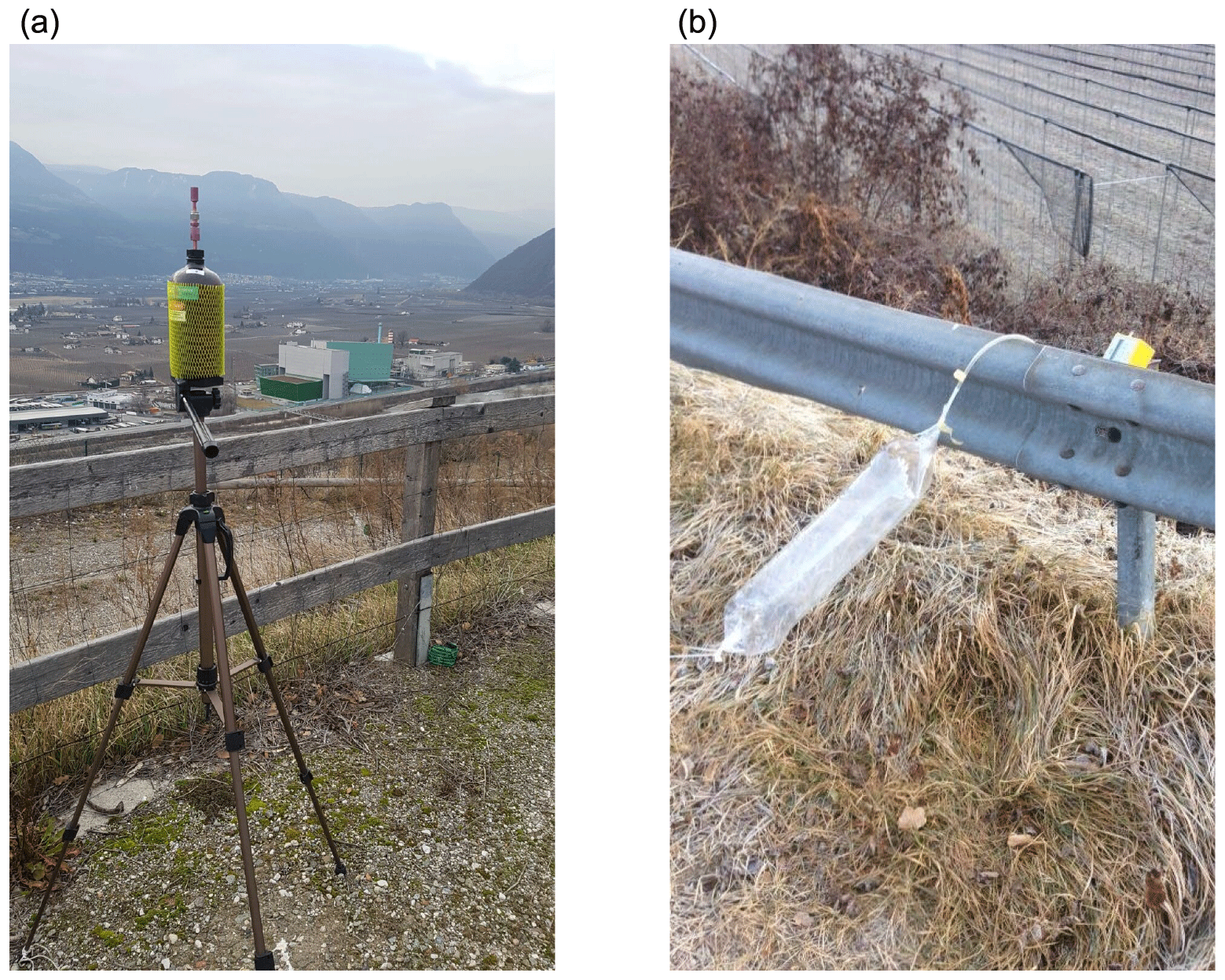
Figure 2Vacuum-filled glass bottle (a) and polyvinyl fluoride (PVF) bag (b) used to collect samples of ambient air. These pictures were taken during the tracer releases of BTEX. On the right of the vacuum bottle, the incinerator of Bolzano can be recognized.
During each release of SF6, 14 sampling teams were located in the field. A crucial issue in the design of the sampling strategy was represented by the definition of the sampling-point positions and their scheduling, i.e., starting time and duration. Given the complex orography of the study area and its related heterogeneous meteorological fields, the samplers distribution could be neither geometrically designed (as for example with concentric circles around the incinerator stack, e.g., Hanna et al., 1986) nor fixed on the basis of the mean wind flow. For these reasons, seven sampling teams were located in the main residential areas, where most of the receptors are concentrated, while the remaining teams were placed in the surroundings of the incinerator, in agreement with the ground concentrations predicted by an operational modeling chain composed of both meteorological and air quality models, specifically set up for the present field campaign. A detailed description of this modeling chain is beyond the purposes of the current paper and will be presented in future related works. Here, its structure and operational use during the experimental campaigns is briefly reported.
The meteorological field inside the Bolzano basin was simulated by means of the Weather Research and Forecasting (WRF) model (Skamarock and Klemp, 2008) through four nested domains, with an increasing horizontal resolution of 13.5 km (northern Italy), 4.5 km (northeastern Italian Alps), 1.5 km (Trentino-Alto Adige) and 0.5 km (Bolzano basin). Moreover, in the innermost domain, observational nudging was adopted, by assimilating all the available data described in Sect. 3.1. Then, the CALMET model (California Meteorological model; Scire et al., 1999) was used to increase the horizontal resolution of the meteorological field simulated by the WRF model up to 200 m, whereas the CALPUFF model (California Puff model; Scire et al., 1999) was adopted to simulate the dispersion processes and the ground concentrations within the study area.
The modeling chain was used
-
48 h before the experiment to pinpoint a first-guess distribution of the samplers on the basis of the predicted meteorological conditions and fallout areas and
-
right before each release, in nowcasting mode, to adjust (if needed) the distribution of the samplers with the updated model output (driven by the most recent assimilated meteorological measurements) and to define the starting time and duration of each sampling.
The resolution adopted for the numerical weather prediction simulations (i.e., 500 m) can fall, in principle, into the so-called gray zone or terra incognita, i.e., those scales where turbulence is neither subgrid nor fully resolved but rather is partially resolved. However, this rather high resolution was necessary to adequately capture the spatial variability of meteorological fields in the Bolzano basin. The CALMET model was used as a physically based interpolator to further increase the horizontal resolution from 500 to 200 m.
3.1 Meteorological measurements
During BTEX, the meteorological field within the study area was monitored by means of 15 surface weather stations (WS in Fig. 1), 1 microwave temperature profiler (MTP; label 3 in Fig. 1), 1 sodar (label 2 in Fig. 1) and 1 Doppler wind lidar (label 4 in Fig. 1).
3.1.1 Surface weather stations
Table 1Surface weather stations (WSs) adopted to monitor the meteorological field during BTEX along with their position (V: valley floor station; S: valley sidewall station), coordinates, altitude and available measurements: air temperature (T); relative humidity (RH); rain (R); atmospheric pressure (P); wind direction (dir); wind intensity (U); wind gust (Ug); global radiation (GR); and sunshine duration (SD). The first column indicates the label of the station shown in Fig. 1.

The 15 surface weather stations are part of the network operated by the Weather Service of the Autonomous Province of Bolzano and are partly located on the valley floors and partly on the sidewalls. These stations, listed in Table 1 and reported in Fig. 1, record every 10 min the following meteorological quantities: air temperature and humidity at , average wind intensity and direction and wind gusts at , rainfall, atmospheric pressure, global radiation, and sunshine duration.
3.1.2 Microwave temperature profiler
Table 2Technical characteristics of the microwave temperature profiler (MTP-5HE) installed at the airfield of Bolzano.
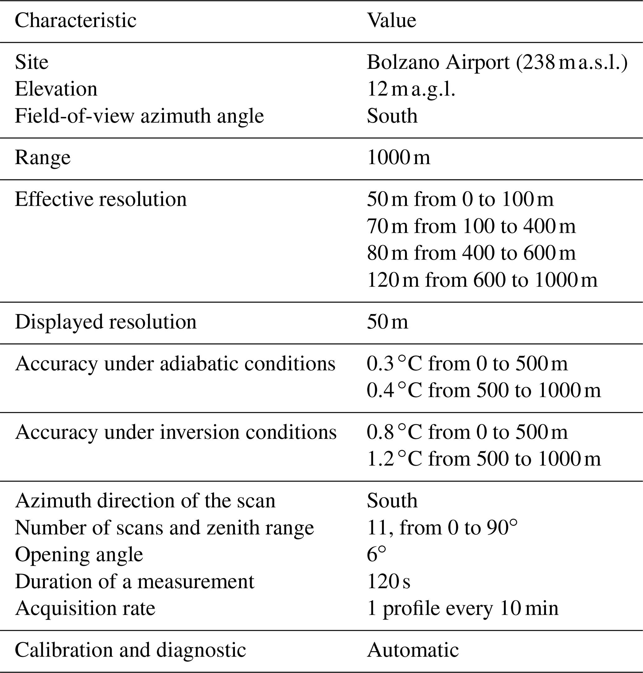
The atmospheric thermal structure inside the basin is constantly monitored by means of an MTP-5HE passive microwave radiometer (manufactured by ATTEX, Russia). The instrument determines the vertical temperature profile at 11 elevation angles (from 0 to 90∘), by measuring the brightness temperature of the molecular oxygen at a frequency of 60 GHz. The device retrieves the air temperature from the measured brightness temperature by solving a Fredholm equation of the first kind (Gaikovich et al., 1992; Troitskii et al., 1993) and interpolates the obtained profile along 21 vertical levels, 50 m spaced. Further information on the functioning of this device can be found in Westwater et al. (1999), Scanzani (2010), Ezau et al. (2013) and Wolf et al. (2014).
The MTP-5HE used during BTEX (technical specifications in Table 2; label 3 in Fig. 1) is operated by the Physical Chemistry Laboratory of the Environmental Protection Agency of the Autonomous Province of Bolzano and is installed at the airfield of Bolzano (46.46∘ N, 11.32∘ E; 238 m a.s.l.), on the roof of a 12 m high building. This device provides the vertical temperature profile from 250 to every 10 min.
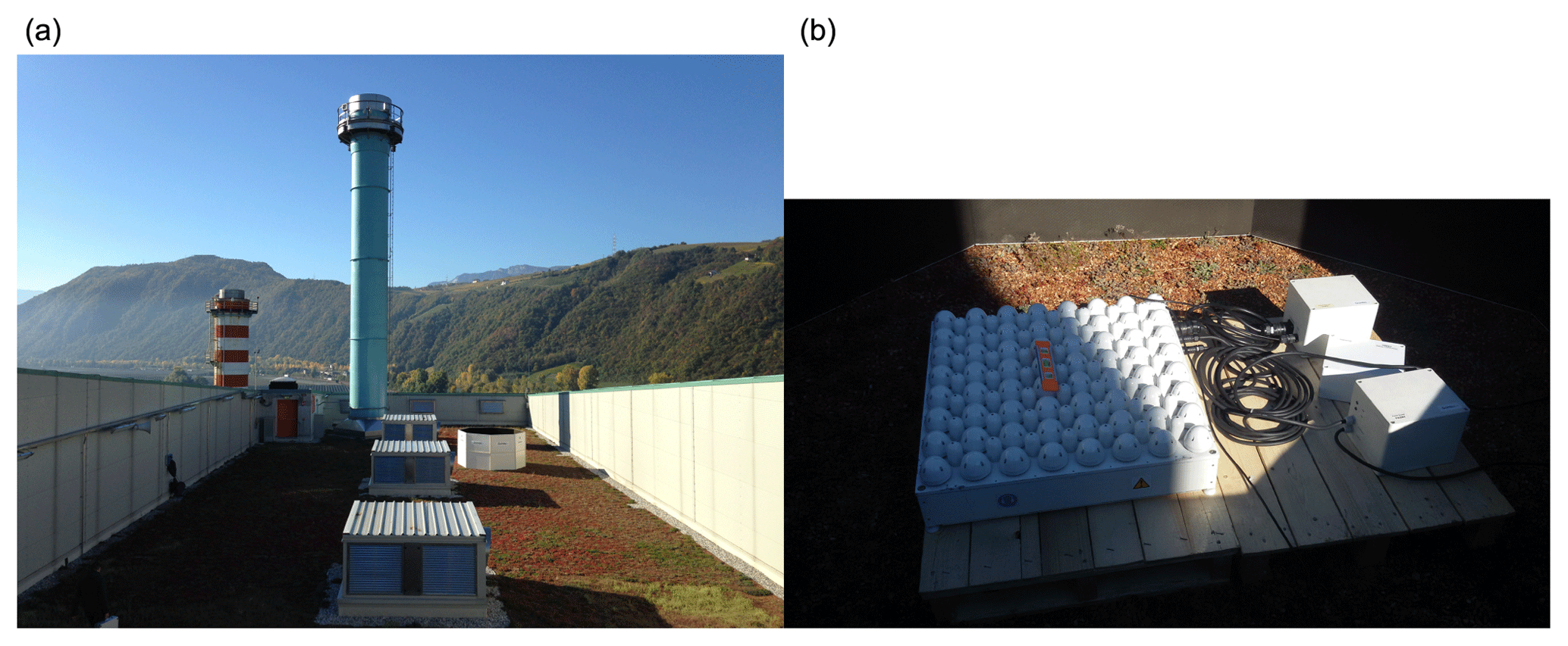
Figure 3A view of the roof of the incinerator of Bolzano during the experimental campaign with the MFAS mini-sodar (a) and the detail of the antenna (b).
3.1.3 Sodar
Wind intensity and direction at the outlet of a stack represent a fundamental input to properly model the fate of pollutants. Accordingly, the wind field at the chimney of the incinerator was monitored by means of an MFAS mini-sodar (manufactured by Scintec, Germany), installed on the roof of the plant at (label 2 in Fig. 1). The sodar, shown in Fig. 3, probed the wind field within a 400 m thick atmospheric layer, from 315 to and with a vertical resolution of 30 m. Raw data were processed by means of the software APRun, provided by Scintec, in order to obtain the vertical profiles of the wind speed components and of the backscatter over an averaging period of 30 min. In particular, the profiles were provided along 38 vertical levels, each spaced by 10 m.
Sodar measurements played a key role in the BTEX project. Indeed, during preliminary analyses preceding the experiment, these measurements allowed us to capture an intense nocturnal wind (wind intensity greater than 10 m s−1) blowing from the northeast. These observations, supported by high-resolution numerical simulations run with the WRF model, allowed us to identify this wind as the drainage flow of the Isarco Valley that, especially under fair-weather conditions, spreads into the Bolzano basin behaving like a thermally driven valley exit jet (Whiteman, 2000).
3.1.4 Doppler wind lidar
The interaction between the valley exit jet of the Isarco Valley and the smoke of the incinerator can strongly affect the pollutant dispersion scenarios within the Bolzano basin. Therefore, a dedicated measurement campaign was performed to monitor this flow, and a Doppler wind lidar (label 4 in Fig. 1) was installed, from 9 January to 5 April 2017 on the roof of a public building at , at the outlet of the Isarco Valley (Fig. 4).
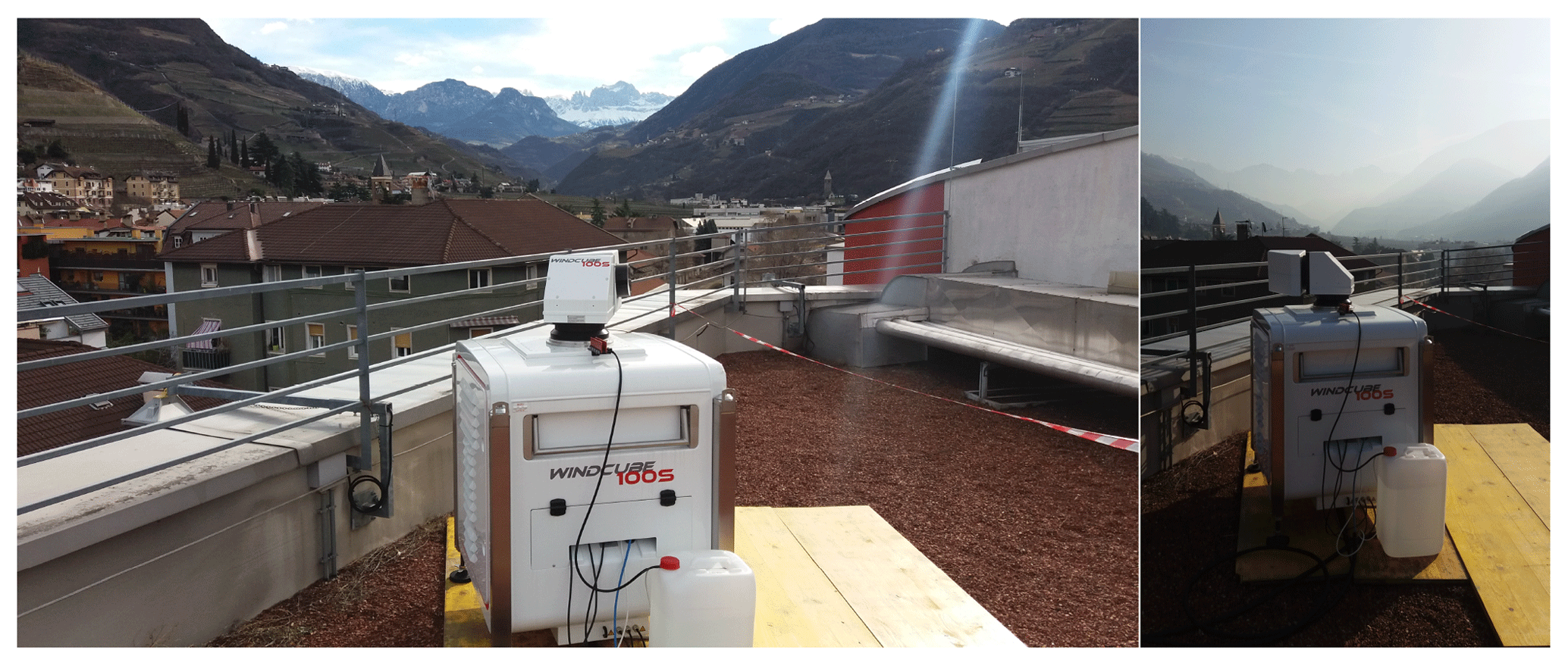
Figure 4The WINDCUBE 100S Doppler wind lidar from Leosphere (France) installed on a roof at In the background is the outlet of the Isarco Valley.
The Doppler wind lidar was a WINDCUBE 100S manufactured by Leosphere (France). This device probes the atmosphere with coherent beams of pulsed, eye-safe electromagnetic waves in the near-infrared domain (wavelength 1.54 µm) and returns measurements of the wind speed component along each line of sight with physical resolutions of 25, 50, 75 or 100 m, up to 319 gates. In the framework of BTEX, the vertical profile of the wind was measured every 5 s by means of the Doppler beam swinging (DBS) technique along 110 vertical levels, 10 m spaced (from 335 to ) and with a vertical resolution of 25 m. These profiles were hourly averaged and assimilated by the modeling system to nowcast both the meteorological variables and the tracer dispersion scenarios.
3.2 Tracer concentration measurements
After each release, samples of ambient air were collected by means of two different technologies: vacuum-filled glass bottles and polyvinyl fluoride bags (hereafter PVF bags). Bottles with a capacity of 1 L were filled by means of a valve, whose calibrated nozzle allowed a constant inflow, thus determining the time required to fill the bottle. In the framework of BTEX, nozzles were calibrated to fill a bottle in 20 or 60 min. The filling of the PVF bags was instead regulated by a suitable air pump controlling the inflow speed.
Different from the online monitoring of SF6 at the incinerator stack, a much higher sensitivity was required for the detection of the tracer concentrations in the samples of ambient air collected in the surroundings of the plant. Accordingly, a triple quadrupole gas chromatography mass spectrometer (TSQ 8000 EVO from Thermo Scientific) with chemical ionization with methane as the reagent gas was used in the laboratory analyses. The obtained sensitivity allowed us to measure down to background levels. Nevertheless, to avoid the influence of the background (see Sect. 2.2.1), SF6 concentrations in the collected samples were quantified at levels above 30 pptv.
The dataset presented in this paper consists of
-
79 samples of SF6 concentrations measured at ground level (according to the descriptions provided in Sects. 2.2.2, 2.2.4, 2.2.3 and 3.2, the volumes of ambient air were collected in 14 different points surrounding the incinerator for the two releases performed during BTEX);
-
time series of meteorological quantities collected by the monitoring network described in Sect. 3.1 (the 15 surface weather stations contributing to the meteorological dataset are listed in Table 1, along with their respective identification label, coordinates, altitude and available observations (x); these data are provided with a time resolution of 10 min and can also be freely downloaded from the open-data web service of the Autonomous Province of Bolzano);
-
temperature profiles measured by means of the microwave temperature profiler (MTP-5HE) every 10 min (these data are provided by the Physical Chemistry Laboratory of the Environmental Agency of the Autonomous Province of Bolzano);
-
sodar measurements, i.e., vertical profiles of mean wind quantities, standard deviations and backscatter, provided every 30 min;
-
Doppler wind lidar vertical profiles of the wind speed components and of the carrier-to-noise ratio, provided every 5 s; and
-
information and working conditions of the incinerator observed during the day of the release, i.e., coordinates and height of the stack and discharge and temperature of the smoke every 30 min (these data can also be freely downloaded from the website of the company operating the plant, eco center S.p.A (https://www.eco-center.it/it/attivita-servizi/ambiente/impianti/impianto-di-termovalorizzazione/reports/reports-giornalieri-795.html, last access: January 2020)).
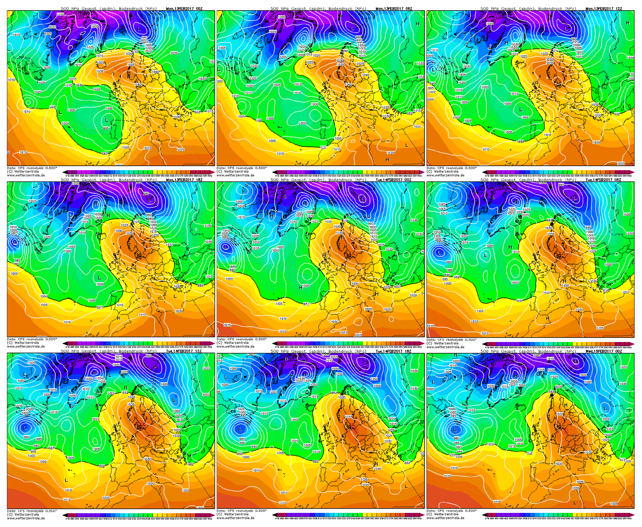
Figure 5CFS reanalyses of geopotential height at 500 hPa from 13 February 2017 00:00 UTC to 15 February 2017 00:00 UTC (https://www.wetterzentrale.de/, last access: January 2020).
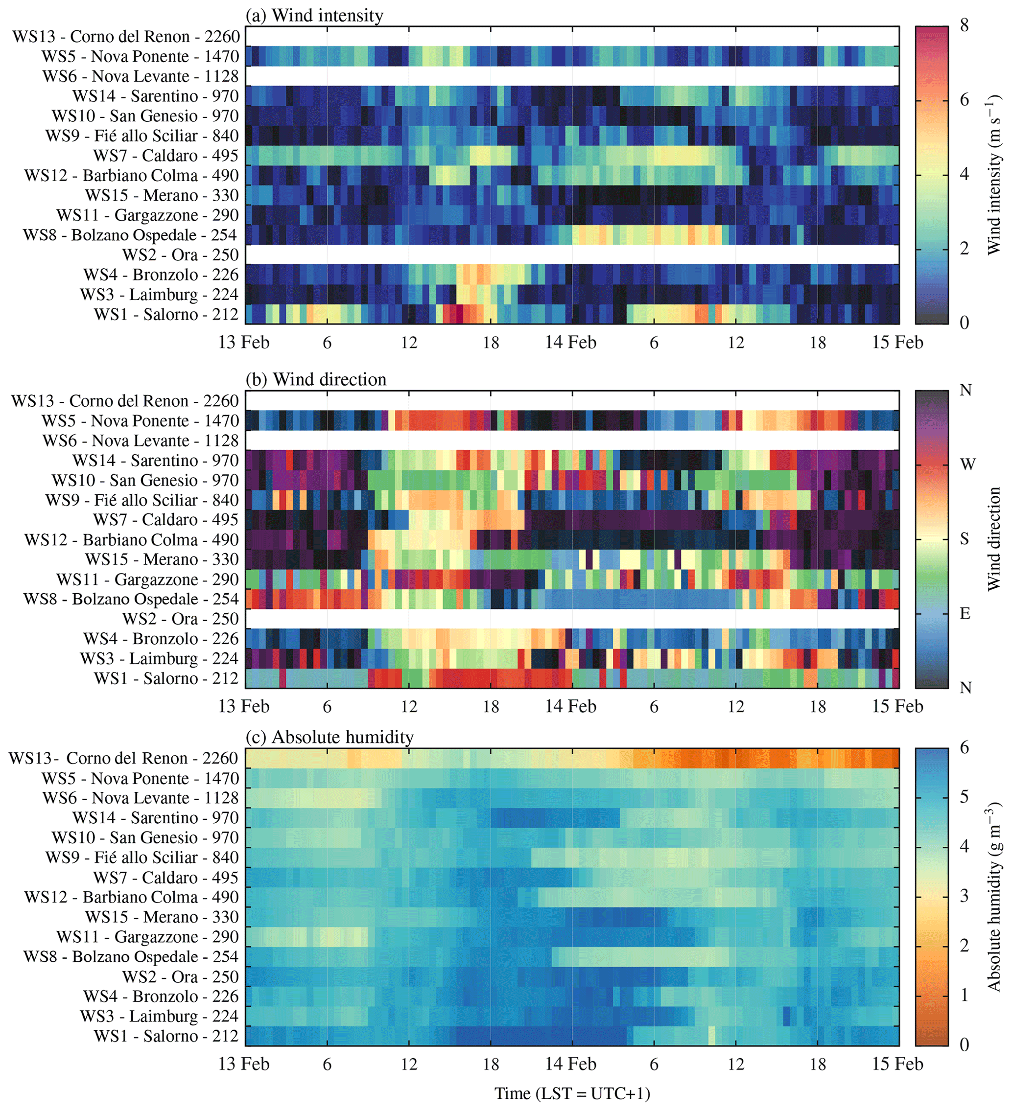
Figure 6Time evolution of the wind intensity (a), the wind direction (b) and the absolute humidity (c) measured by the 15 surface weather stations used during BTEX (see Table 1). The absolute humidity was computed from data of relative humidity, air temperature and atmospheric pressure. Weather stations are ordered according to their elevation, with the aim of displaying a pseudovertical distribution of the observed quantities.
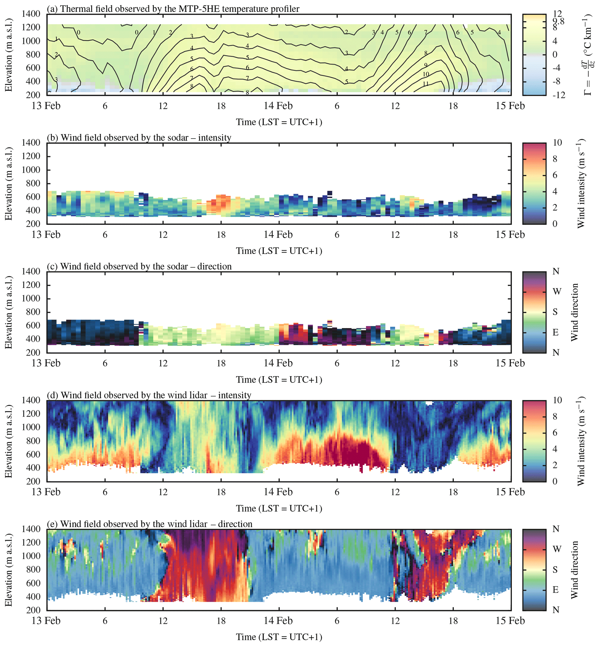
Figure 7Time–height distribution of the thermal field (a) and of the wind fields measured by the sodar (b–c) and by the Doppler wind lidar (d–e) inside the Bolzano basin.
5.1 Weather conditions
Releases of SF6 were performed on 14 February 2017, when over northern Italy a high-pressure system was present with very weak synoptic winds. The evolution of the synoptic conditions from 13 February 00:00 UTC to 15 February 00:00 UTC is reported in Fig. 5, in terms of maps of geopotential height at 500 hPa as simulated by the reanalyses of the Climate Forecast System (CFS) model (source: https://www.wetterzentrale.de/). On 13 February, the weakening of a low-pressure system above the Iberian Peninsula induced southwestern synoptic winds blowing over the study area, which channeled into the valleys. Especially during the afternoon and the evening of 13 February, these synoptic winds interacted with the local circulations by strengthening the up-valley winds, as observed by the surface weather stations (Fig. 6a) and by both the sodar and the Doppler wind lidar (Fig. 7b–e). As a further effect, the synoptic winds transported moist air into the valleys. Indeed, the distributions of absolute humidity shown in Fig. 6c display an increase of the moisture content in the afternoon of 13 February at all the weather stations used in BTEX (Table 1).
During the night of 13 and 14 February, the moist air produced low-level clouds that covered the sky above the study area and inhibited the radiative cooling of the ground. Indeed, as confirmed by the microwave temperature profiler (Fig. 7a), this night was warmer than the previous one, and no significant ground-based temperature inversions developed. The absence of synoptic forcing instead allowed the development of thermally driven circulations. However, the wind regimes captured by the surface weather stations on the floor of the Adige Valley at Bronzolo (WS4 in Fig. 1) and at Gargazzone (WS11, Fig. 1) appear to be different from the one observed in the Isarco Valley at Barbiano Colma (WS12 in Fig. 1). Indeed, as shown in Fig. 6a and b, the winds observed at Bronzolo (WS4) and Gargazzone (WS11) were weak and with intensities of less than 1 m s−1, while at Barbiano Colma (WS12) the down-valley wind was much stronger, with intensities of around 3 m s−1. In particular, the topographic constraints of the Isarco Valley and of its outlet into the Bolzano basin determined the acceleration of the winds blowing from this valley, thus allowing the development of a thermally driven valley exit jet, whose evolution was observed by the Doppler wind lidar. The time–height plots of the wind intensity (Fig. 7d) and of the wind direction (Fig. 7e) measured by the Doppler wind lidar reveal the valley exit jet blowing from the east after 21:00 LST (UTC+1) with intensities of around 5 m s−1 in a layer about 400 m deep. During the night, the wind became stronger in an increasingly deep layer until the early morning (14 February 09:00 LST), when it reached its maximum intensity, exceeding 13 m s−1. Then, as is typical of these phenomena (Banta et al., 1995; Chrust et al., 2013), the jet abruptly ceased around 11:00 LST. The valley exit jet was also observed at ground level by the weather stations at Bolzano Ospedale (WS8 in Fig. 1) and Caldaro (WS7 in Fig. 1). Indeed, in the morning of 14 February, the weather station at Bolzano Ospedale (WS8, Fig. 6a, b) recorded a strong easterly wind exceeding 5 m s−1. The weather station at Caldaro (WS7, Fig. 6a, b) instead measured a northerly wind of around 3 m s−1 that intensified from 06:00 to 09:00 LST (wind speed above 4 m s−1), in agreement with the behavior of the valley exit jet. The footprint of the valley exit jet can also be observed in the time series of absolute humidity (Fig. 6c) measured by the previously mentioned surface weather stations, i.e., Barbiano Colma (WS12), Bolzano Ospedale (WS8) and Caldaro (WS7). Indeed, in these series, a significant reduction of absolute humidity is observed during the valley exit jet event. Therefore, it seems reasonable to assume that the valley exit jet advected drier air from the upper valleys into the basin. After noon on 14 February, both the sodar and the Doppler wind lidar observed a weak up-valley wind (around 2 m s−1) rising from the south in the Adige Valley. Also at ground level, the surface weather stations (Fig. 6a and b) recorded very weak winds, with intensities of around 1 m s−1.
5.2 Dispersion patterns
The two releases of SF6 were carried out to investigate the fallout areas of the tracer under different conditions of atmospheric stability and blowing winds, according to the release strategy (Sect. 2.2.2) and the sampling strategy (Sect. 2.2.4) described above. These data can be used to evaluate the spatial patterns of the tracer in the target area and its evolution in 14 different points. Table 3 summarizes the main characteristics of these releases. In particular, Table 3 reports the timetables and the masses of the tracer released, the metadata concerning the incinerator smoke, the number of sampling teams and the number of collected samples. Furthermore, information regarding the coordinates of the sampling points and the collected samples (sampling devices and time resolution) is reported in Tables 4 and 5 for the first and the second release, respectively. During both the releases, instantaneous samples of ambient air were also collected outside the laboratory, located in the Bolzano city center, and immediately analyzed as described in Sect. 3.2. These measurements allowed for monitoring the presence of the tracer in the atmosphere in quasi-real-time, thereby enabling verification of the effectiveness of the releases.
Table 3Summary of the two releases performed during BTEX (VB: vacuum-filled glass bottles; TB: PVF bags).

Table 4Geographical coordinates of the sampling points (SP) along with number of samples of ambient air collected during the first release of BTEX (VB: vacuum-filled glass bottle; TB: PVF bags). The numbers after VB and TB indicate the duration in minutes of the sampling.
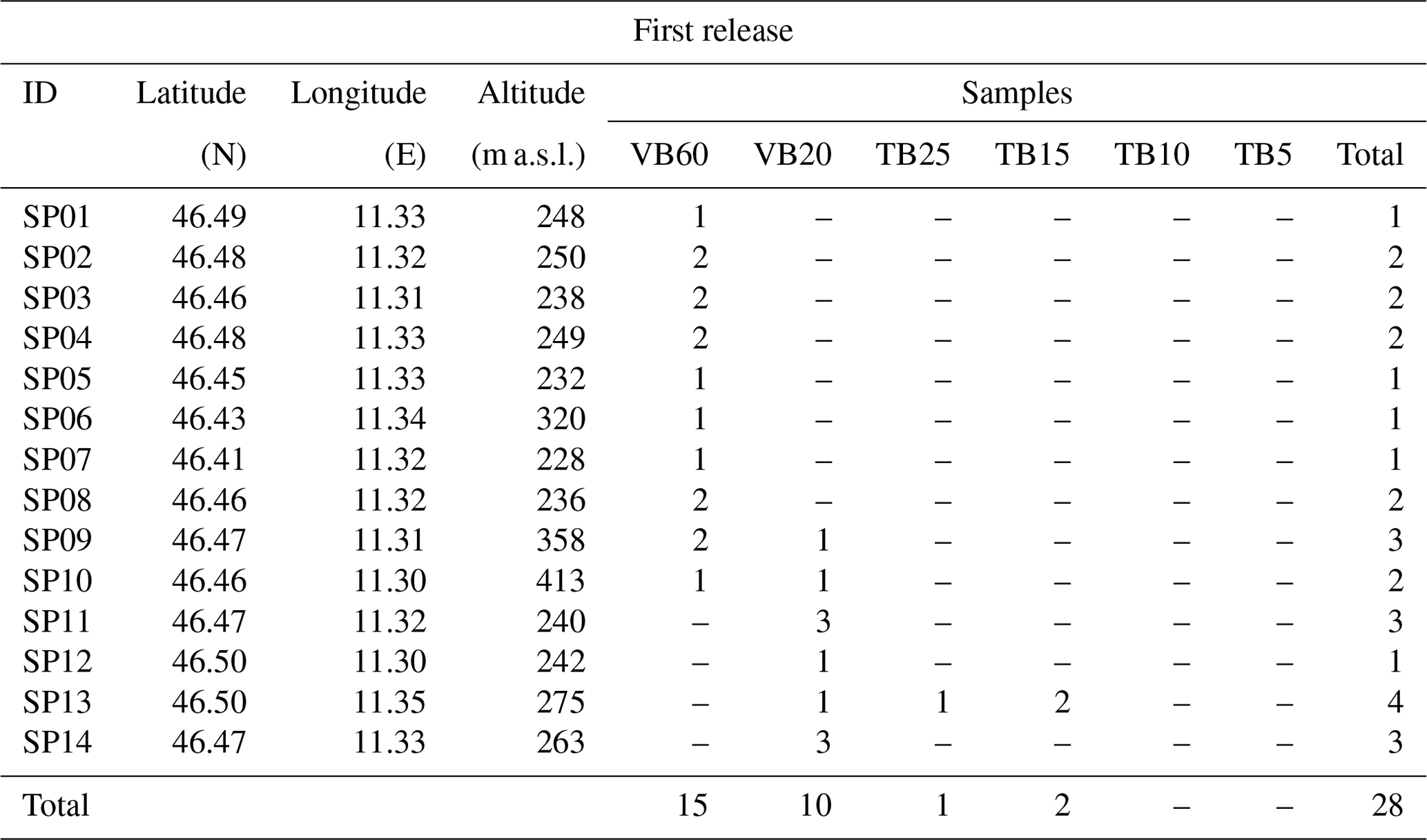
Table 5Geographical coordinates of the sampling points (SP) along with number of samples of ambient air collected during the second release of BTEX (VB: vacuum-filled glass bottle; TB: PVF bags). The numbers after VB and TB indicate the duration in minutes of the sampling.
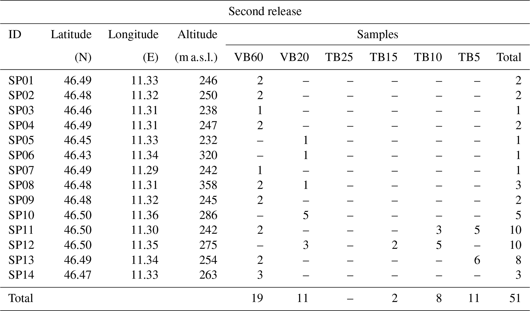
Figure 8 provides a graphical overview of the dataset, by representing the time evolution of the concentrations measured by the sampling teams during each release (gray areas). In particular, in view of describing the spatial patterns of the tracer along the axis of the Adige Valley, i.e., in agreement with the observed wind regime, the sampling points are ordered according to their latitude, i.e., from south (below) to north (above), while the horizontal black line marks the latitude of the incinerator. Each box corresponds to one sample: the length of the box fits the timing and the duration of the sampling, whereas the color corresponds to the measured concentration. Specifically, blue boxes correspond to samples in which the tracer concentration was lower than the detectability limit of the laboratory analyses, i.e., 30 pptv. White areas, instead, correspond to periods without samplings.
The first release of BTEX was carried out in the early morning, in order to evaluate the dispersion of pollutants in a stable nocturnal atmosphere with a light down-valley wind (i.e., blowing from north to south; see for example the weather station at Bronzolo (WS4) in Fig. 6a and b). In this case, the valley exit jet from the Isarco Valley, being confined north of the incinerator within the Bolzano basin, did not interact with the released smoke. These atmospheric conditions suggested the envisaging of a weak dispersion of the tracer and a fallout area south of the incinerator, in the Adige Valley. The tracer release started at 07:00 LST and ended 1 h later, whereas the sampling activity started at 08:30 LST and continued until 10:45 LST. During this release, the 14 sampling teams collected a total of 28 samples of ambient air at the points represented in the maps in Fig. 9. Figure 9 shows the positions of the sampling teams and the tracer concentrations at four different times (see times with arrows in Fig. 8). At the beginning of the sampling period (45 min after the end of the release; Fig. 9a), only one team northeast of the incinerator observed a concentration of SF6 significantly different from the background (0.03–0.1 ppb), whereas at 09:15 LST the tracer was observed south of the incinerator in the Adige Valley, with concentrations ranging between 0.1 and 0.5 ppb (Fig. 9b). These findings confirm that the transport of the tracer due to the advection by the mean wind dominated over turbulent dispersion, and therefore the fallout of the tracer at surface level was slower. After 09:30 LST, thanks to the heating of the ground and the onset of a weak up-valley wind (WS3 and WS4 in Fig. 6a and b), tracer concentrations increased also in the area surrounding the incinerator (Fig. 9c and d), where a maximum concentration of 1.19 ppb was observed (Fig. 9d). However, consistent with the observed wind speed and direction, the tracer never reached the town of Bolzano.
The second release started at 12:45 LST and ended at 14:15 LST, in order to investigate the dispersion processes under a weakly unstable atmosphere and an up-valley wind rising in the Adige Valley (see WS3, WS4, WS8 and WS11 in Fig. 6a and b). Under these atmospheric conditions, the mixing is usually more efficient, and a faster fallout of the tracer, north of the incinerator, was expected. Therefore, samples of ambient air were collected from 13:10 LST (still during the release) until 16:30 LST. Indeed, a concentration of 11.96 ppb was observed north of the incinerator at 13:15 LST (Fig. 10a), i.e., 30 min after the beginning of the release. At the end of the release (14:15 LST; Fig. 10b), the up-valley wind moved the smoke of the plant northward, and significant concentrations of SF6 were measured west of Bolzano, inside the basin, while very low concentrations were observed south of the incinerator. After 30 min (Fig. 10c), the tracer spread into the basin, even if high concentrations were still observed west of Bolzano. Background concentrations of SF6 ranging between 0.2 and 0.5 ppb, as shown in Fig. 10a, were also found, as a consequence of the persistence of the tracer released in the morning.
At the end of this second release a total of 51 samples were collected by means of both vacuum-filled glass bottles and PVF bags.
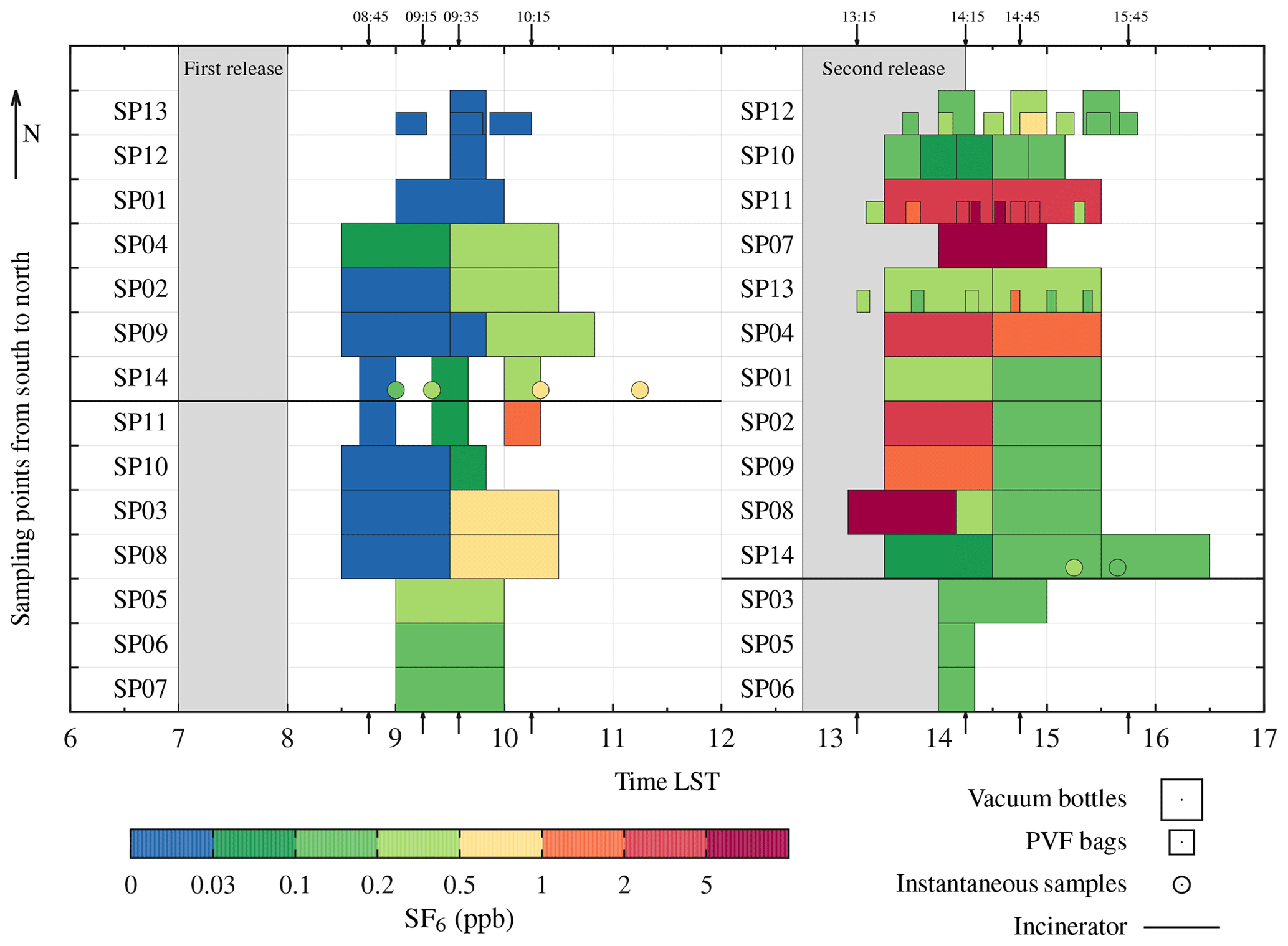
Figure 8Tracer concentrations measured on 14 February 2017 after each release. Air samples were collected by means of vacuum-filled glass bottles (large rectangles) and PVF bags (small rectangles). In addition, instantaneous samples of air (circles) were analyzed. The sampling points are listed from north to south, while the two horizontal black lines indicate the latitude of the incinerator. The arrows at the top and bottom of the graph indicate reference time stamps (LST) for Figs. 9 and 10.
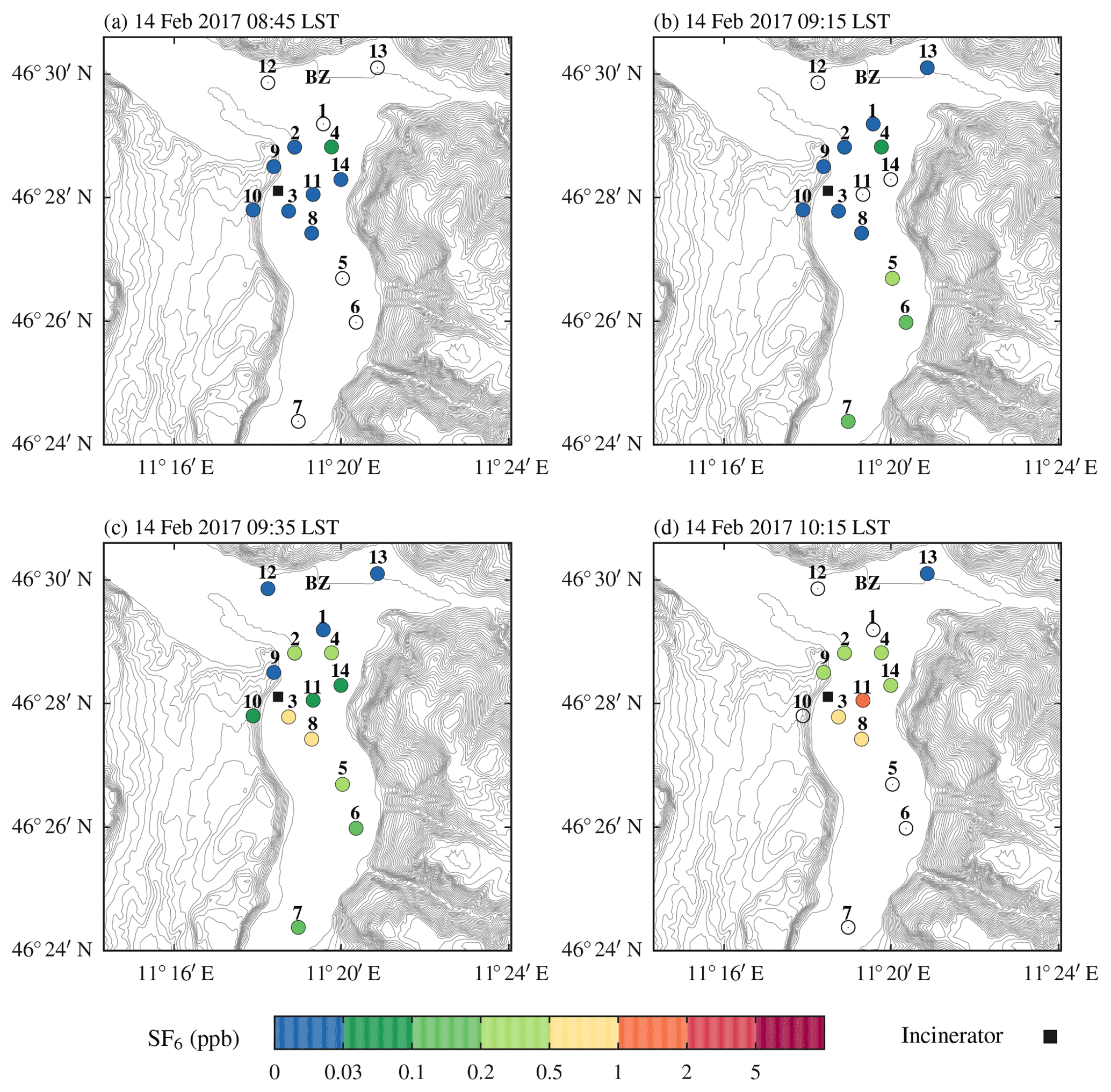
Figure 9Spatial distribution of the tracer concentrations measured during the release performed in the morning of 14 February 2017. The position of the city of Bolzano is indicated on the map with the label BZ.
All data presented in this paper are publicly available at World Data Center PANGAEA (https://doi.org/10.1594/PANGAEA.898761, Falocchi et al., 2019).
The Bolzano Tracer EXperiment (BTEX) represents one of the few experiments available in the literature performed over complex mountainous terrain to evaluate dispersion processes by means of controlled tracer releases and under well-documented meteorological conditions. The obtained dataset presented in this paper is the result of a 3-year project during which a great effort was made to properly design, organize and manage all the activities connected to the measurement campaigns. Indeed, preliminary investigations and also ad hoc measurement campaigns were performed to identify the most suitable monitoring network (Sect. 3.1) able to properly capture the local circulation patterns characterizing the meteorology of the Bolzano basin. At the same time, the release of the tracer through the stack of the incinerator was designed. This task included (i) the selection of the tracer (Sect. 2.2.1) and a representative day for the study area (Sect. 2.2.3); (ii) the definition of the injection of the tracer to ensure and monitor the steadiness of the release (Sect. 2.2.2); (iii) the definition of the devices used to collect samples of ambient air at ground level (Sect. 2.2.4) and of the required laboratory analysis to measure the tracer concentrations (Sect. 3.2).
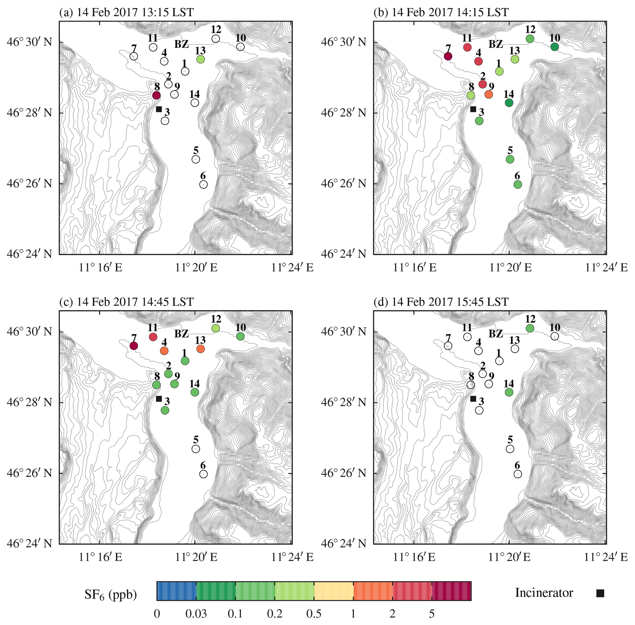
Figure 10Spatial distribution of the tracer concentrations measured during the release performed in the afternoon of 14 February 2017. The position of the city of Bolzano is indicated in the map with the label BZ.
On 14 February 2017 two tracer releases were performed. The collected dataset contains 79 samples of tracer ground concentrations, collected during each release in 14 different locations of the study area and at different times. The complex orography of the study area and its related heterogeneous meteorological fields did not allow for a regular distribution of the sampling points around the incinerator, e.g., in concentric circles. Therefore, seven sampling points were located in the main residential areas neighboring the incinerator, while the other seven sampling points were placed in agreement with the fallout areas of the tracer, as predicted by a modeling chain specifically set up for the purposes of the study and composed of both meteorological and dispersion models. In particular, for a proper interpretation of the output of the modeling chain, a key role was played by the expertise gained by the modeling team on the typical meteorological processes characterizing the study area. The adopted strategy allowed us to capture the space–time variability of the tracer at ground level. More details on the numerical experiments carried out to simulate the tracer dispersion can be found in Tomasi et al. (2019).
The dataset is completed with a detailed description of the meteorological field, provided by 15 surface weather stations, 1 microwave temperature profiler, 1 sodar and 1 Doppler wind lidar. Specifically, the meteorological data cover a period of 48 h starting from 13 February 2017 00:00 LST in order to provide a more complete description of the meteorological processes within the study area.
The uniqueness of BTEX makes the collected dataset a useful benchmark for testing dispersion models in complex terrain.
MF led the writing of the paper and prepared all figures and tables. WT wrote the section on chemical measurements. DZ revised preliminary versions of the manuscript. All authors contributed to suggesting ideas and reviewing the paper. All authors contributed to the design and planning of the experiment and participated in the field campaigns. WT provided the required tools for air samples collection, instructed the team of observers and performed all the laboratory analyses. MF, LG, ET and GA managed the sodar and the Doppler wind lidar operations. GA, ET and LG contributed to the setup of the modeling chain and operated it during the field campaigns. MF collected all the data, both from the field experiment and from permanent observational facilities in the target area and surroundings; organized the dataset; and created its publication on World Data Center PANGAEA. DZ, as principal investigator, managed the overall execution of the project, including partners' involvement and commitment, from the initial concept to the conclusion, and suggested the preparation of the present paper.
The authors declare that they have no conflict of interest.
The authors acknowledge Marco Palmitano (eco center S.p.A) and Bruno Eisenstecken (eco center S.p.A), who encouraged and strongly supported this study, also by renting the Doppler wind lidar. The authors are also grateful to all the personnel of eco center S.p.A., Eco-Research s.r.l., the Environmental Agency of the Autonomous Province of Bolzano and the Mario Negri Institute for Pharmacological Research for participating in the measurement activities during the releases. The Weather Service of the Autonomous Province of Bolzano is acknowledged for kindly providing data from its weather stations. The Environmental Agency of the Autonomous Province of Bolzano, Massimo Guariento and Luca Verdi are kindly acknowledged for data from the microwave temperature profiler.
This paper was edited by Scott Stevens and reviewed by two anonymous referees.
Allwine, K. J. and Flaherty, J. E.: Joint Urban 2003: Study overview and instrument locations, Tech. rep., Pacific Northwest National Laboratory (PNNL), Richland, WA (US), 2006. a, b
Ambrosetti, P., Anfossi, D., Cieslik, S., Graziani, G., Grippa, G., Marzorati, R. L. A., Stingele, A., and Zimmermann, H.: The TRANSALP-90 Campaign. The second tracer release experiment in a sub-alpine valley, Tech. Rep. Technical Report EUR 15952 EN, Commission of the European Communities, 1994. a
Banta, R. M., Olivier, L. D., Neff, W. D., Levinson, D. H., and Ruffieux, D.: Influence of canyon-induced flows on flow and dispersion over adjacent plains, Theor. Appl. Climatol., 52, 27–42, https://doi.org/10.1007/BF00865505, 1995. a
Bowne, N. E., Londergan, R. J., Murray, D. R., and Borenstein, H. S.: Overview, results, and conclusions for the EPRI Plume Model Validation and Development Project: Plains site, Electric Power Research Institute Rep. EA-3074, Project, 1616–1, 1983. a
Britter, R. E., Di Sabatino, S., Caton, F., Cooke, K. M., Simmonds, P. G., and Nickless, G.: Results from three field tracer experiments on the neighbourhood scale in the city of Birmingham UK, Water Air Soil Poll. Focus, 2, 79–90, 2002. a, b
Camuffo, D., De Bortoli, M., and Gaglione, P.: Tests on atmospheric diffusion with tracers in an urban area, Tech. Rep. 108, NATO CC MS, 1979. a, b
Chrust, M. F., Whiteman, C. D., and Hoch, S. W.: Observations of Thermally Driven Wind Jets at the Exit of Weber Canyon, Utah, J. Appl. Meteorol. Climatol., 52, 1187–1200, https://doi.org/10.1175/JAMC-D-12-0221.1, 2013. a
Clawson, K. L., Carter, R. G., Lacroix, D. J., Biltoft, C. A., Hukari, N. F., Johnson, R. C., Rich, J. D., Beard, S. A., and Strong, T. W.: Joint Urban 2003 (JU03) SF6 atmospheric tracer field tests, Tech. rep., NOAA Technical Memorandum OAR ARL-254, Air Resources Laboratory, Idaho Falls, Idaho, 237 pp., 2005. a
Cramer, H. E., Record, F. A., and Vaughan, H. C.: The study of the diffusion of gases or aerosols in the lower atmosphere, Tech. rep., MIT Department of Meteorology, Boston, 1958. a
Darby, L. S., Allwine, K. J., and Banta, R. M.: Nocturnal low-level jet in a mountain basin complex. Part II: Transport and diffusion of tracer under stable conditions, J. Appl. Meteorol. Climatol., 45, 740–753, 2006. a, b
de Franceschi, M. and Zardi, D.: Study of wintertime high pollution episodes during the Brenner–South ALPNAP measurement campaign, Meteorol. Atmos. Phys., 103, 237–250, https://doi.org/10.1007/s00703-008-0327-2, 2009. a
De Wekker, S. F. J., Kossmann, M., Knievel, J. C., Giovannini, L., Gutmann, E. D., and Zardi, D.: Meteorological Applications Benefiting from an Improved Understanding of Atmospheric Exchange Processes over Mountains, Atmosphere, 9, 371, https://doi.org/10.3390/atmos9100371, 2018. a, b
Doran, J. C. and Horst, T. W.: An evaluation of Gaussian plume–depletion models with dual–tracer field measurements, Atmos. Environ. (1967), 19, 939—951, https://doi.org/10.1016/0004-6981(85)90239-2, 1985. a
Doran, J. C., Allwine, K. J., Flaherty, J. E., Clawson, K. L., and Carter, R. G.: Characteristics of puff dispersion in an urban environment, Atmos. Environ., 41, 3440–3452, 2007. a, b
Emberlin, J. C.: A sulphur hexafluoride tracer experiment from a tall stack over complex topography in a coastal area of Southern England, Atmos. Environ. (1967), 15, 1523–1530, 1981. a, b
Ezau, I. N., Wolf, T., Miller, E. A., Repina, I. A., Troitskaya, Y. I., and Zilitinkevich, S. S.: The analysis of results of remote sensing monitoring of the temperature profile in lower atmosphere in Bergen (Norway), Russian Meteorology and Hydrology, 38, 715–722, https://doi.org/10.3103/S1068373913100099, 2013. a
Falocchi, M., Tirler, W., Giovannini, L., Tomasi, E., Antonacci, G., and Zardi, D.: Tracer concentrations and meteorological observations from the Bolzano Tracer EXperiment (BTEX), https://doi.org/10.1594/PANGAEA.898761, 2019. a, b
Fiedler, F.: Proposal of a Subproject: “Transport of Air Pollutants over Complex Terrain (TRACT)”, EUREKA Environmental Project, Karlsruhe, 1989. a
Fiedler, F. and Borrell, P.: TRACT: Transport of Air Pollutants over Complex Terrain, 239–283, Springer Berlin Heidelberg, Berlin, Heidelberg, https://doi.org/10.1007/978-3-642-59718-3_11, 2000. a
Gaikovich, K. P., Kadygrov, E. N., Kosov, A. S., and Troitskii, A. V.: Thermal sounding of the atmospheric boundary layer at the center of the oxygen absorption line, Radiofizika, 35, 130—136, 1992. a
Giovannini, L., Antonacci, G., Zardi, D., Laiti, L., and Panziera, L.: Sensitivity of Simulated Wind Speed to Spatial Resolution over Complex Terrain, Energy Procedia, 59, 323–329, european Geosciences Union General Assembly 2014, EGU Division Energy, Resources & the Environment (ERE), 2014. a
Giovannini, L., Laiti, L., Serafin, S., and Zardi, D.: The thermally driven diurnal wind system of the Adige Valley in the Italian Alps, Q. J. Roy. Meteorol. Soc., 143, 2389–2402, 2017. a
Giovannini, L., Ferrero, E., Karl, T., Rotach, M. W., Staquet, C., Trini Castelli, S., and Zardi, D.: Atmospheric pollutant transport over complex terrain: challenges and needs for improving air quality measurements and modelling, Atmosphere, in review, 2020. a
Gromke, C., Buccolieri, R., Di Sabatino, S., and Ruck, B.: Dispersion study in a street canyon with tree planting by means of wind tunnel and numerical investigations–evaluation of CFD data with experimental data, Atmos. Environ., 42, 8640–8650, 2008. a, b
Gryning, S. E. and Lyck, E.: Elevated source SF6-tracer dispersion experiments in the Copenhagen area. Preliminary results II, in: Proceedings of the seminar on radioactive releases and their dispersion in the atmosphere following a hypothetical reactor accident, Risoe, 22–25 April 1980, 1980. a, b
Gryning, S. E. and Lyck, E.: The Copenhagen tracer experiments: Reporting of measurements, Tech. rep., Risø-R-1054(rev.1)(EN), Riso National Laboratory, Roskilde, Denmark, 75 pp., 2002. a
Hanna, S. R., Weil, J., and Paine, R.: Plume model development and evaluation., Tech. Rep. Report Number D034-500, Electric Power Research Institute, Palo Alto, CA, 1986. a, b
Kalthoff, N., Horlacher, V., Corsmeier, U., Volz Thomas, A., Kolahgar, B., Geiß, H., Möllmann-Coers, M., and Knaps, A.: Influence of valley winds on transport and dispersion of airborne pollutants in the Freiburg-Schauinsland area, J. Geophys. Res.-Atmos., 105, 1585–1597, 2000. a, b
Manca, G.: GreenHouse Gases concentration-2017., Tech. rep., European Commission, Joint Research Centre (JRC) [Dataset] PID: http://data.europa.eu/89h/jrc-abcis-ghg-2017 (last access: January 2020), 2017. a
Min, I. A., Abernathy, R. N., and Lundblad, H. L.: Measurement and analysis of puff dispersion above the atmospheric boundary layer using quantitative imagery, J. Appl. Meteorol., 41, 1027–1041, 2002. a
Nieuwstadt, F. T. M. and van Duuren, H.: Dispersion experiments with SF6 from the 213 m high meteorological mast at Cabauw in the Netherlands., in: Proceedings of the 4th Symposium on Turbulence, Diffusion and Air Pollution, Reno, Nevada, 15–18 January, 34–40, American Meteorological Society, Boston, MA, 1979. a
Nodop, K., Connolly, R., and Girardi, F.: The field campaigns of the European Tracer Experiment (ETEX): overview and results, Atmos. Environ., 32, 4095–4108, https://doi.org/10.1016/S1352-2310(98)00190-3, 1998. a
Ragazzi, M., Tirler, W., Angelucci, G., Zardi, D., and Rada, E. C.: Management of atmospheric pollutants from waste incineration processes: the case of Bozen, Waste Manage. Res., 31, 235–240, https://doi.org/10.1177/0734242X12472707, 2013. a
Rigby, M., Mühle, J., Miller, B. R., Prinn, R. G., Krummel, P. B., Steele, L. P., Fraser, P. J., Salameh, P. K., Harth, C. M., Weiss, R. F., Greally, B. R., O'Doherty, S., Simmonds, P. G., Vollmer, M. K., Reimann, S., Kim, J., Kim, K.-R., Wang, H. J., Olivier, J. G. J., Dlugokencky, E. J., Dutton, G. S., Hall, B. D., and Elkins, J. W.: History of atmospheric SF6 from 1973 to 2008, Atmos. Chem. Phys., 10, 10305–10320, https://doi.org/10.5194/acp-10-10305-2010, 2010. a
Rotach, M. W. and Zardi, D.: On the boundary–layer structure over highly complex terrain: Key findings from MAP, Q. J. Roy. Meteorol. Soc., 133, 937–948, https://doi.org/10.1002/qj.71, 2007. a
Scire, J. S., Robe, R. B., Fernau, M. E., and Yamartino, R.: A User's Guide for the CALMET Meteorological Model (Version 5), Earth Tech, Inc., Concord. MA, 1999. a
Scire, J. S., Strimaitus, D., and Yamartino, R.: A User's Guide for the CALPUFF Dispersion Model (Version 5), Earth Tech, Inc., Concord, MA, 2000. a
Scanzani, F.: Ground based passive microwave radiometry and temperature profiles, in: Remote Sensing for Wind Energy, edited by: Pena, A. and Hasager, C. B., 260–275, Technical Univ. of Denmark, DTU Wind Energy, DTU Risoe Campus, Roskilde, Denmark, 2010. a
Serafin, S., Adler, B., Cuxart, J., De Wekker, S. F. J., Gohm, A., Grisogono, B., Kalthoff, N., Kirshbaum, D. J., Rotach, M. W., Schmidli, J., Stiperski, I., Večenaj, Ž., and Zardi, D.: Exchange Processes in the Atmospheric Boundary Layer Over Mountainous Terrain, Atmosphere, 9, 102, https://doi.org/10.3390/atmos9030102, 2018. a, b
Sivertsen, B.: Tracer Experiments to Estimate Diffusive Leakages and to Verify Dispersion Models, 255–268, Springer Netherlands, Dordrecht, https://doi.org/10.1007/978-94-009-2939-5_20, 1988. a
Skamarock, W. C. and Klemp, J. B.: A time-split nonhydrostatic atmospheric model for weather research and forecasting applications, J. Comput. Phys., 227, 3465–3485, https://doi.org/10.1016/j.jcp.2007.01.037, 2008. a
Tomasi, E., Giovannini, L., Zardi, D., and de Franceschi, M.: Optimization of Noah and Noah_MP WRF Land Surface Schemes in Snow-Melting Conditions over Complex Terrain, Mon. Weather Rev., 145, 4727–4745, https://doi.org/10.1175/MWR-D-16-0408.1, 2017. a
Tomasi, E., Giovannini, L., Falocchi, M., Zardi, D., Antonacci, G., Ferrero, E., Bisignano, A., Alessandrini, S., and Mortarini, L.: Dispersion Modeling Over Complex Terrain in the Bolzano Basin (IT): Preliminary Results from a WRF–CALPUFF Modeling System, in: Air Pollution Modeling and its Application XXV, edited by: Mensink, C. and Kallos, G., 157–161, Springer International Publishing, Cham, 2018. a
Tomasi, E., Giovannini, L., Falocchi, M., Antonacci, G., Jimenez, P. A., Kosovic, B., Alessandrini, S., Zardi, D., Delle Monache, L., and Ferrero, E.: Turbulence parameterizations for dispersion in sub–kilometer horizontally non-homogeneous flows, Atmos. Res., 228, 122–136, https://doi.org/10.1016/j.atmosres.2019.05.018, 2019. a, b, c
Troitskii, A. V., Gaikovich, K. P., Gromov, V. D., Kadygrov, E. N., and Kosov, A. S.: Thermal sounding of the atmospheric boundary layer in the oxygen absorption band center at 60 GHz, IEEE T. Geosci. Remote, 31, 116–120, https://doi.org/10.1109/36.210451, 1993. a
Van Dop, H., Addis, R., Fraser, G., Girardi, F., Graziani, G., Inoue, Y., Kelly, N., Klug, W., Kulmala, A., Nodop, K., and Pretel, J.: ETEX: a European tracer experiment; observations, dispersion modelling and emergency response, Atmos. Environ., 32, 4089–4094, 1998. a
Westwater, E. R., Han, Y., Irisov, V. G., Leuskiy, V., Kadygrov, E. N., and Viazankin, S. A.: Remote Sensing of Boundary Layer Temperature Profiles by a Scanning 5-mm Microwave Radiometer and RASS: Comparison Experiments, J. Atmos. Ocean. Tech., 16, 805–818, https://doi.org/10.1175/1520-0426(1999)016<0805:RSOBLT>2.0.CO;2, 1999. a
Whiteman, C. D.: Morning transition tracer experiments in a deep narrow valley, J. Appl. Meteorol., 28, 626–635, 1989. a, b
Whiteman, C. D.: Mountain Meteorology: Fundamentals and Applications, Oxford University Press, New York, 2000. a, b
Wolf, T., Esau, I., and Reuder, J.: Analysis of the vertical temperature structure in the Bergen valley, Norway, and its connection to pollution episodes, J. Geophys. Res.-Atmos., 119, 10645–10662, https://doi.org/10.1002/2014JD022085, 2014. a
Wood, C. R., Arnold, S. J., Balogun, A. A., Barlow, J. F., Belcher, S. E., Britter, R. E., Cheng, H., Dobre, A., Lingard, J. J. N., Martin, D., Neophytou, M. K., Petersson, F. K., Robins, A. G., Shallcross, D. E., Smalley, R. J., Tate, J. E., Tomlin, A. S., and White, I. R.: Dispersion experiments in central London: the 2007 DAPPLE project, B. Am. Meteorol. Soc., 90, 955–970, 2009. a, b
Zannetti, P., Carboni, G., and Ceriani, A.: Avacta II Model Simulations of Worst-Case Air Pollution Scenarios in Northern Italy, 113–121, Springer US, Boston, MA, https://doi.org/10.1007/978-1-4757-9125-9_8, 1986. a, b
Zardi, D. and Whiteman, C. D.: Diurnal Mountain Wind Systems, in: Mountain Weather Research and Forecasting: Recent Progress and Current Challenges, edited by: Chow, F. K., De Wekker, S. F. J., and Snyder, B. J., 35–119, Springer Netherlands, Dordrecht, 2013. a, b
Zimmermann, H.: Field phase report of the TRACT field measurement campaign, Tech. rep., Garmisch-Partenkirchen: EUROTRAC Int. Sci. Secr., 1995. a