the Creative Commons Attribution 4.0 License.
the Creative Commons Attribution 4.0 License.
 | 17 Feb 2020
A national dataset of 30 m annual urban extent dynamics (1985–2015) in the conterminous United States
Xuecao Li
Zhengyuan Zhu
Wenting Cao
Dynamics of the urban extent at fine spatial and temporal resolutions over large areas are crucial for developing urban growth models and achieving sustainable development goals. However, there are limited practices of mapping urban dynamics with these two merits combined. In this study, we proposed a new method to map urban dynamics from Landsat time series data using the Google Earth Engine (GEE) platform and developed a national dataset of annual urban extent (1985–2015) at a fine spatial resolution (30 m) in the conterminous United States (US). First, we derived the change information of urbanized years in four periods that were determined from the National Land Cover Database (NLCD), using a temporal segmentation approach. Then, we classified urban extents in the beginning (1985) and ending (2015) years at the cluster level through the implementation of a change vector analysis (CVA)-based approach. We also developed a hierarchical strategy to apply the CVA-based approach due to the spatially explicit urban sprawl over large areas. The overall accuracy of mapped urbanized years is around 90 % with the 1-year tolerance strategy. The mapped urbanized areas in the beginning and ending years are reliable, with overall accuracies of 96 % and 88 %, respectively. Our results reveal that the total urban area increased by about 20 % during the period of 1985–2015 in the US, and the annual urban area growth is not linear over the years. Overall, the growth pattern of urban extent in most coastal states is plateaued over the past three decades while the states in the Midwestern US show an accelerated growth pattern. The derived annual urban extents are of great use for relevant urban studies such as urban area projection and urban sprawl modeling over large areas. Moreover, the proposed mapping framework is transferable for developing annual dynamics of urban extent in other regions and even globally. The data are available at https://doi.org/10.6084/m9.figshare.8190920.v2 (Li et al., 2019c).
- Article
(6913 KB) -
Supplement
(1325 KB) - BibTeX
- EndNote


The rapid global urbanization causes environmental, ecological, and public concerns for human beings for sustainable development goals (SDGs) (Rodriguez et al., 2018). Globally, urban areas, commonly defined as the space dominated by the built environment (e.g., buildings, roads, and runways) from remote sensing, only account for a tiny fraction of the Earth's surface (Schneider et al., 2010); however, they are home to most of the global economy, population, energy consumption, and greenhouse gas emissions (Solecki et al., 2013). According to the latest World Urbanization Prospects (United Nations, 2019), more than 50 % of the world's population lives in urban areas, and this percentage will increase to 66 % by the middle of this century. Moreover, most urban population growth would likely to occur in developing regions, where the realization of SDGs faces more challenges because of potential risks from thermal environment change caused by the urban heat island (Peng et al., 2012), degradation of urban ecosystem services (Li et al., 2017; Irwin and Bockstael, 2007), energy consumption with changed environment and human activities (Güneralp et al., 2017; Zhou et al., 2014; Alberti et al., 2017), and public health concerns (Gong et al., 2012; Luber et al., 2014). Therefore, understanding the pathway of urban sprawl (i.e., expansion of the geographic extent of urban area) and the development of advanced urban growth models are highly needed for adapting and mitigating potential risks under future urbanization (Li and Gong, 2016a; Weng, 2012).
The datasets of urban extent dynamics at the fine spatial (e.g., 30 m) and temporal (e.g., annual) resolutions are the key to capturing the rate, trend, and stage of urbanization for a better understanding of this process (Zhang et al., 2014). Such datasets can provide fine information about the urban form (e.g., layout, geometry, and distribution), which can be further used for relevant studies such as urban energy consumption (Chen et al., 2011), biodiversity in urban ecosystem (Andersson and Colding, 2014), and air pollutant emissions (Fan et al., 2018). In addition, the relationship between urban dynamics and annual socioeconomic development (e.g., population and gross domestic product) can help to better understand the reasons behind urbanization (Seto et al., 2002; Xie and Weng, 2017). Finally, the long temporal span (e.g., decades) of urban dynamics can capture a relatively complete process of urban sprawl with different stages (Li et al., 2019a; Gong et al., 2019, 2020; Cao et al., 2020). The information of long-term urban dynamics is valuable in developing urban growth models, such as investigating the generation and propagation of errors (or uncertainties) in urban sprawl models (Santé et al., 2010; Li and Gong, 2016a). However, current mapping approaches that focus on multitemporal (e.g., decade and half-decade) urban extent are limited to reflect the process of urban sprawl (e.g., acceleration or deceleration) of cities and explain their differences caused by demographic and socioeconomic drivers (Sexton et al., 2013).
Urban extent mapping at fine spatial and temporal resolutions, especially over large areas, is still lacking, although urban extent maps with a variety of spatial and temporal resolutions have been developed. For example, there are several global urban extent products such as those from the nighttime light (NTL) data (1 km) (Zhou et al., 2015, 2018; Xie and Weng, 2016), the Moderate Resolution Imaging Spectroradiometer (MODIS) data (500 m) (Schneider et al., 2010), and even the fine-resolution Landsat data (30 m) (Chen et al., 2015; Gong et al., 2013; Liu et al., 2018). However, these existing multitemporal national or global urban extent maps were generally produced separately in each period, with limited consideration of the temporal consistency of urban growth (Li et al., 2015; Song et al., 2016; Shi et al., 2017).
There are several challenges in mapping urban extent at fine spatial and temporal resolutions over large areas. First, land use and cover changes in urban domains are complicated, with the interclass conversions and multiphase changes before urbanization or during the posturbanization period (Li and Gong, 2016b; Lu and Weng, 2004). For example, various land cover types such as vegetation, water, and barren can be potentially converted to built-up areas, and such a conversion may experience multiple phases, e.g., from highly vegetated land to lightly vegetated or barren, and then eventually to built-up areas with posturbanization changes. Second, durations of land surface change introduced by urbanization are different across regions; that is, urban sprawl may occur within a short period or last for a couple of years in different regions (Song et al., 2016; Kennedy et al., 2010).
In general, two approaches have been used to derive spatiotemporally consistent urban extent maps from high spatial and temporal satellite observations. One is improving the classified urban time series using postprocessing techniques (Liu and Cai, 2012; Li et al., 2015); the other one is identifying the change information using the continuous time series data of relevant indicators such as the vegetation index (Huang et al., 2010; Kennedy et al., 2010). The first method requires intensive labor for collecting training samples for classification and specific postprocessing techniques (Gong et al., 2013, 2019; Chen et al., 2015; Liu and Cai, 2012), which is challenging and time-consuming for regional and global mapping over a long temporal span. The second one poses a new challenge for managing, manipulating, and analyzing the massive amount of time series data over large areas.
Due to these challenges in mapping urban dynamics at fine spatial and temporal resolutions over large areas, the development of a generalized and efficient mapping approach is in high demand. In this study, we mapped the annual dynamics (1985–2015) of urban extent in the conterminous United States (US) by developing a generalized and efficient mapping approach on the state-of-the-art Google Earth Engine (GEE) platform. The remainder of this paper describes the study area and data (Sect. 2), the proposed national-mapping approach (Sect. 3), the results with discussion (Sect. 4), the data availability (Sect. 5), and concluding remarks (Sect. 6).
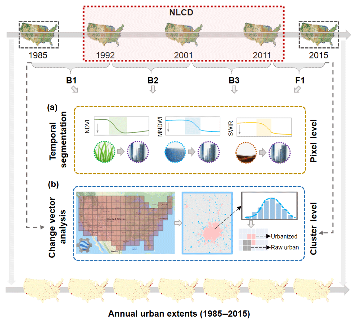
Figure 1The proposed framework for mapping annual urban extent dynamics in the conterminous US through the detection of the urbanized year at the pixel level using the temporal segmentation approach (a) and classifying urbanized areas at the cluster level in periods B1 and F1 using the change vector analysis (b) (Basemap data© 2019 Google).
Landsat time series data on the GEE platform, spanning from 1985–2015, are the primary data source for mapping annual urban extent in this study. The advent of GEE is designed for planetary-scale studies using different sources of satellite images (Gorelick et al., 2017; Li et al., 2019b), and it is a good choice for mapping projects over large areas. In this study, we used multiple L1T-level Landsat surface reflectance products, including the Thematic Mapper (TM), the Enhanced Thematic Mapper Plus (ETM+), and the Operational Land Imager (OLI). These products have been corrected for the radiometric, topographic, and atmospheric effects (Masek et al., 2006). All clean-sky pixels were used to composite the time series data for analyses, with clouds and their shadows removed. In total, around 460 000 Landsat scenes were used for the conterminous US over the past three decades.
The National Land Cover Database (NLCD) and nighttime light data are ancillary datasets in this study. The NLCD provides multitemporal urban maps in 1992, 2001, 2006, and 2011 (Homer et al., 2015; Xian et al., 2009), which were used as the reference urban areas in these years. The NLCD has been widely used for its reliable performance at the national scale (Wickham et al., 2010, 2017). In this study, we derived the urban extent map in 1992 using the NLCD 1992/2001 retrofit land cover change product, so that all urban extents derived from the NLCD in different years (i.e., 1992, 2001, 2006, and 2011) are comparable (Fry et al., 2009). In addition, nighttime light images of the Visible Infrared Imaging Radiometer Suite (VIIRS) were used to delineate the potential urban cluster after 2011 (Li and Zhou, 2017).
In this study, we developed a new framework with a unique hierarchical strategy for mapping annual urban extents in large areas on the GEE platform using long-term Landsat observations (Fig. 1). First, we grouped the study period (1985–2015) into four periods, namely B1 (1985–1992), B2 (1992–2001), B3 (2001–2011), and F1 (2011–2015), based on the available NLCD. For Landsat time series data in each period, we detected the urbanized years at the pixel level by implementing a temporal segmentation approach (Li et al., 2018) (Fig. 1a). Second, given that NLCD only provides urban extent from B2 to B3, we classified urbanized areas at the cluster level in the periods B1 and F1 using a change vector analysis (CVA)-based approach. We developed a hierarchical strategy to implement the CVA-based approach due to the spatially explicit urban sprawl over large areas. That is, the CVA-based approach was applied in potential urban clusters (derived from VIIRS data) in each grid (around 250 km × 250 km), according to the size of potential urban clusters (Fig. 1b). Details of each procedure are presented in the following sections.
3.1 Detection of urbanized years
We preprocessed the raw Landsat time series data before implementing the temporal segmentation approach. We systematically corrected the OLI surface reflectance data to make them consistent with other sensors (i.e., TM and ETM+) as suggested by Roy et al. (2016). After that, we generated the normalized difference vegetation index (NDVI), the modified normalized difference water index (MNDWI), and the shortwave infrared (SWIR) reflectance. These three indexes can well represent vegetation, water, and bare lands, respectively, and are the primary conversion sources to urbanized areas (Li and Gong, 2016b). The annual maximal NDVI was used to represent the growth of vegetation because the NDVI has a distinctive seasonal pattern and the greenest season varies over different biomes, e.g., January–March in the western US and June–August in the central US. The annual mean values of MNDWI and SWIR from all observations except for the winter time were used to composite the annual time series data.
We implemented the temporal segmentation approach for each urbanized pixel in four periods (i.e., B1, B2, B3, and F1). These urbanized pixels during each period were identified using urban extent maps derived from NLCD and classified results in B1 and F1 using the CVA-based approach. Within each period, we identified the starting (P1) and ending (P2) years of change using the temporal segmentation approach, according to the overall trend of the indicators (i.e., NDVI, MNDWI, and SWIR). For urbanization from vegetation, the indicator of NDVI shows a decreasing trend (Fig. 2a), while curves of MNDWI and SWIR show increasing trends (Fig. 2b). In this temporal segmentation method, we first applied a linear regression to the annual time series data of three indicators (i.e., NDVI, MNDWI, and SWIR) and then determined these two turning points (i.e., P1 and P2) according to their annual residuals to the regression-based trend line. If the overall trend of NDVI is decreasing, the years with the largest residuals above and below the regression-based trend line were identified as P1 and P2, respectively, and vice versa (Fig. 2). The change year derived from the indicator with the largest change magnitude (i.e., change between P1 and P2) was identified as the final result. In addition, the duration of change is the difference of years between P1 and P2. More details about the temporal segmentation can be found in Li et al. (2018).

Figure 2Illustration of the temporal segmentation approach using indicators with decreasing (NDVI) (a) or increasing (MNDWI and SWIR) (b) trends.
3.2 Classification of urbanized areas before 1992 and after 2011
We classified urbanized areas in periods B1 (1985–1992) and F1 (2011–2015) using a CVA-based approach at the national level (Fig. 1b). Urbanized areas of two middle periods (i.e., B2 and B3) were directly obtained from NLCD. Results from the temporal segmentation approach (i.e., change magnitude within each period) were used to identify urbanized areas in the CVA-based approach in the beginning (B1) and ending (F1) periods. Full time series data were used in our CVA-based approach, which is different from the commonly used approach based on a pair of images in two periods (Xian et al., 2009; Yu et al., 2016). The change magnitude (ΔV) was calculated using three indicators (Eq. 1). Compared to the six-spectral-band information of Landsat, the three indicators show similar or even better performance in capturing the change magnitude (Fig. S1 in the Supplement), as well as in providing the information of conversion sources of urbanized areas. Pixels with a large ΔV were regarded as potentially changed areas. We identified these potentially changed areas using a multithreshold approach because different conversions have different thresholds of ΔV (Eq. 2).
where CVj is the status of change (i.e., 1 is change and 0 is no change) for cover type j; μj and σj are the mean and standard deviation of ΔVj; t1 and t2 are the turning years of P1 (before change) and P2 (after change), respectively; and α is an adjustable parameter that was set as 1.5 in this study as suggested by Morisette and Khorram (2000).
We implemented the CVA-based approach within urban masks in the first (B1) and last (F1) periods. For B1, the urban extent of NLCD 1992 was used as a potential urban mask before 1992. For the period F1, an approximate urban extent derived from VIIRS data in 2015 (Li et al., 2018) was used as a potential urban boundary for classification. Within the derived urban boundary, we classified urban areas in 2015 using urban pixels sampled from NLCD 2011. Finally, we derived urbanized areas in the period F1, using the potential change areas from the CVA approach, the urban boundary from NTL data, and the urban extent from NLCD 2011. Pseudo-changes that are not relevant to the urban sprawl were removed during this process. More details about the CVA-based approach can be found in Li et al. (2018).
3.3 A hierarchical strategy on the GEE
We developed a hierarchical strategy to implement the CVA-based approach at the national level. This strategy enables us to detect urbanized areas over large areas with spatially explicit patterns of urban sprawl. In this strategy, we grouped all potential urban clusters into two categories using a size filter of 100 km2 (Fig. S2) for implementing different thresholds in the CVA-based approach to derive urbanized areas (Fig. 3). For those large clusters (i.e., larger than 100 km2), we isolated each of them as an independent spatial unit and applied the CVA-based approach to them. For the remaining small urban clusters within the same grid, we treated them as an integrated unit to derive urbanized areas.
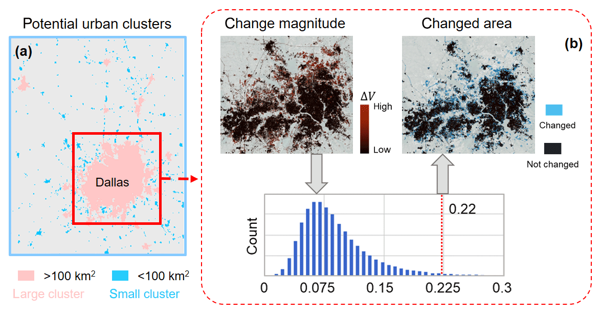
Figure 3An illustration of the CVA-based approach. An example grid with potential urban clusters including Dallas, Texas, for implementing the CVA-based approach (a). An example of the CVA-based approach in the cluster of Dallas, Texas (b). The change magnitude is the difference of three indicators (i.e., NDVI, MNDWI, and SWIR) before and after the urbanized year, and the changed areas are pixels with magnitudes greater than the determined threshold (μ+1.5σ) from the histogram (dotted red line). μ and σ are the mean and standard derivation of change magnitudes in the potential urban cluster.
4.1 Annual urban growth
The annual growth of urban areas varies across years in the conterminous US, which cannot be revealed by the NLCD (Fig. 4). Overall, the average growth rate at the national scale is around 1000 km2 yr−1 during 1985–2015. The total increment is about 31 000 km2, which is around 20 % relative to the urban area in 1985 (Fig. 4a). Our results provide more details of urban dynamics according to the annual growth rate (km2 yr−1) of urban areas, compared to the growth rate (km2 yr−1) of the NLCD in each period (Fig. 4b). The mean growth rates of NLCD are 1015, 1512, and 929 km2 yr−1 during the periods of 1992–2001, 2001–2006, and 2006–2011, respectively. However, the annual dynamics within each period are notably different. In general, there are notably decreasing trends of growth during the periods of 1997–2001 and 2007–2010 and a profound increasing trend during 2004–2006. Particularly, the decreasing trend during 2006–2011 is the most significant, with a total decrease from 1380 km2 yr−1 in 2007 to 520 km2 yr−1 in 2010, which is likely caused by the financial crisis around 2008.

Figure 4Annual growth of urban areas in the conterminous US (1985–2015) (a) and their annual growth rates (km2 yr−1) compared to the NLCD in the three periods (shadow frames) of 1992–2001, 2001–2006, and 2006–2011 (b).
The annual growth of urban areas is different across states. There is an overall increasing trend in the early years and a decreasing trend in the latter years in period of 2001–2011 (Fig. 5). The mean growth rate in all states is 25 km2 yr−1. Texas (TX), Florida (FL), and California (CA) are three states with the highest growth rates, which are 117, 93, and 80 km2 yr−1, respectively. In general, in most states, their relative changes of annual growth in urban area are higher than the mean growth rate of NLCD in the early years. After that, their relative changes of annual growth are below the mean growth rate. This trend is consistent with NLCD results, with a declined mean growth rate of around 40 % during the period of 2006–2011 relative to 2001–2006 (Fig. 4b). It is worth noting that NLCD in 2006 was not used in our mapping approach. The comparison of the urban area growth during 2001–2006 shows a good agreement between our results and NLCD (Fig. S3). Therefore, the NLCD in 2006 independently indicates that our approach can well capture the dynamic of urban areas.

Figure 5State-based relative change of annual growth of urban areas compared to the mean growth rate of NLCD during the period of 2001–2011 (Basemap data© 2019 Esri).
A distinctive urban area growth was observed for cities with a rapid population growth. We chose the top 10 cities in the US based on the population growth rate during 2010–2017 (Fig. 6). Most of them are in the southern and the eastern US, such as TX, FL, and North Carolina (NC). Overall, the growth of urban areas in these top 10 cities is significant. The rank-based urban area growth agrees well with the result from population growth (Fig. S4). For example, there is a remarkable urban sprawl around 2006–2015 in the Village city (FL), which is also the city with the fastest population growth among the top 10.
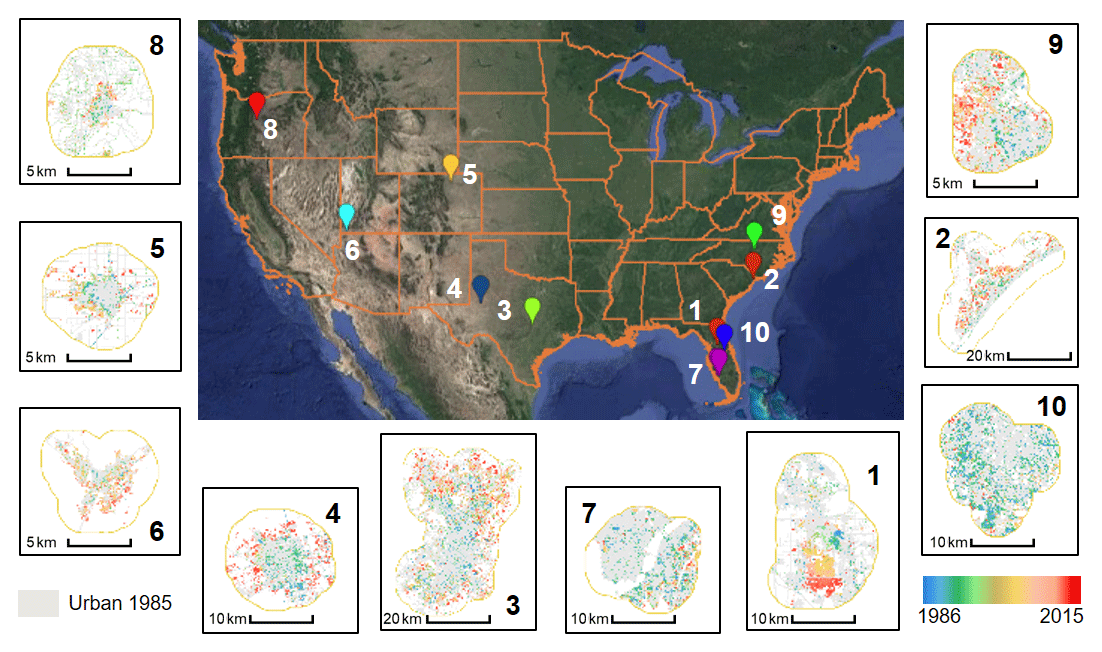
Figure 6An illustration of urban area growth in the top 10 fast-growing cities in the US according to the population growth during 2010–2017. (1) Village (Florida), (2) Myrtle Beach (South Carolina/North Carolina), (3) Round Rock (Texas), (4) Midland (Texas), (5) Greeley (Colorado), (6) St. George (Utah), (7) Fort Myers (Florida), (8) Redmond (Oregon), (9) Raleigh (North Carolina), and (10) Orlando (Florida) (Basemap data© 2019 Google).
4.2 Long-term patterns of urban growth
Our annual urban extent data reveal different long-term patterns of urban growth across states in the US during the past three decades. We calculated the percentage of urban area growth relative to the base year 1985 for each state from 1986 to 2015. States show different patterns (i.e., convex or concave hull) according to the time series of relative change (Fig. 7a). As such, we defined two urban area growth patterns by comparing the derived time series curve to the reference line (Fig. 7b). If the curve of urban area growth was overall above the reference line (e.g., Missouri, MO), then we regarded this pattern as a plateaued growth; on the contrary, it belongs to an accelerated growth pattern (e.g., Arizona, AZ). In general, urban area growth patterns in most coastal states are plateaued, and states in the south and the midwestern US show an accelerated growth pattern in general (Fig. 7c). In particular, the relatively accelerated growth of urban areas over the past three decades in agricultural states such as Iowa (IA), North Dakota (ND), and South Dakota (SD) challenges the sustainable development of agriculture system. Also, the annual urban areas over a long term indicate that the urban area growth is not linear over the years, although the linear growth of urban areas was widely used in urban sprawl modeling, if only the coarse-temporal-resolution urban extent data are available (Li et al., 2014; Sexton et al., 2013).
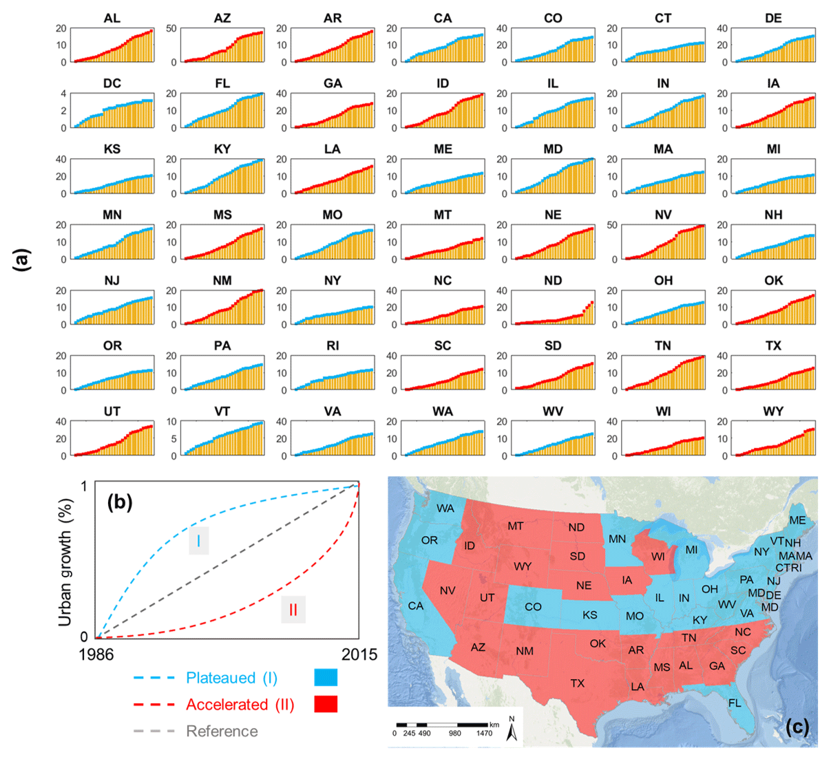
Figure 7Urban area growth patterns over the past three decades of each state in the US (a), the proposed conceptual model (b), and the classified urban area growth types (c) (Basemap data© 2019 Esri).
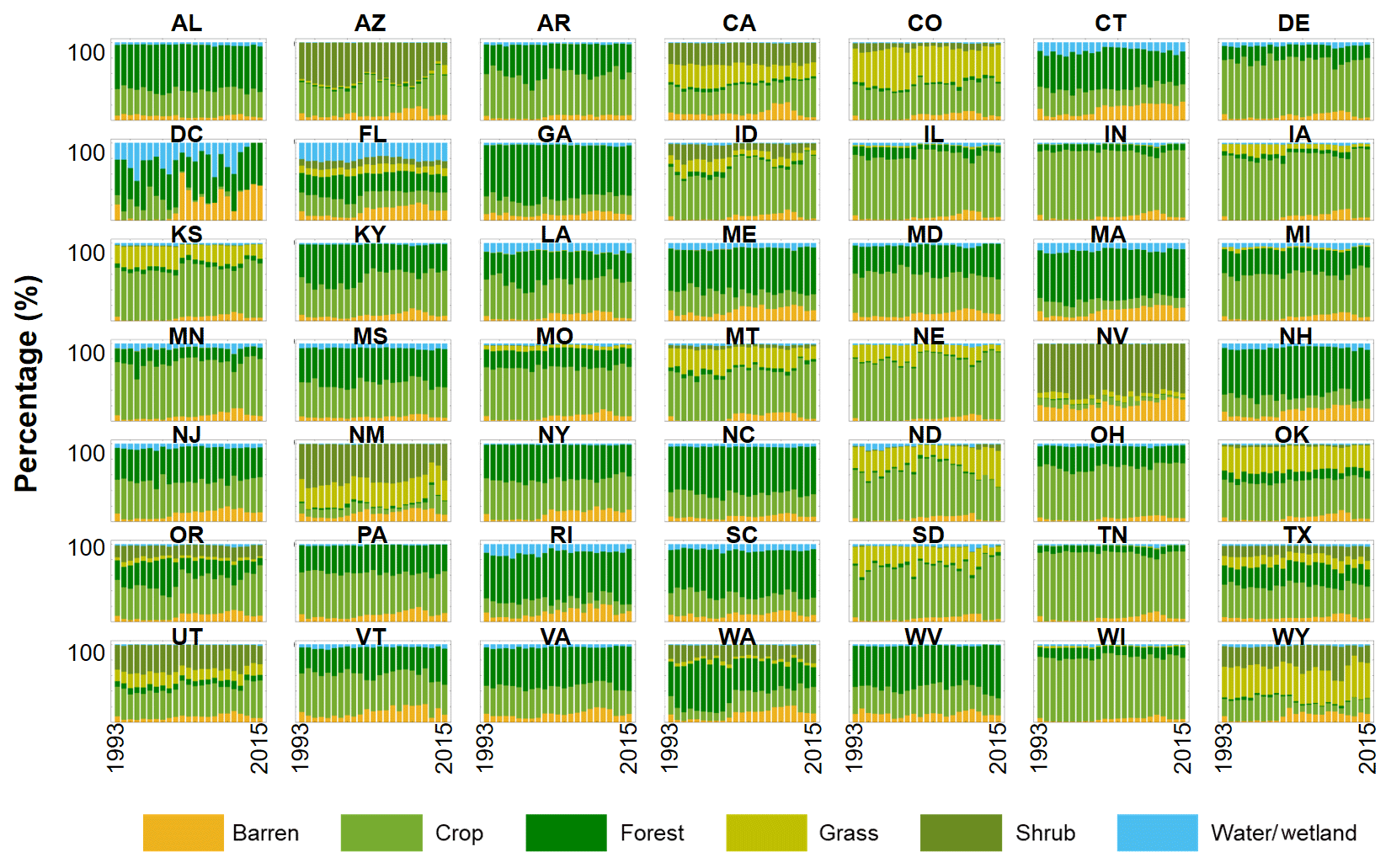
4.3 Conversion sources of urbanized areas
The primary conversion sources of urbanized areas are different across states and change over time (Fig. 8). Most urbanized areas were converted from cropland and forest within a relatively short duration (i.e., 1–3 years) (Fig. S5–S6). Overall, vegetation (i.e., cropland, forest, grass, and shrub) is the dominant source of urbanized areas over all the states and years. In particular, the cropland is the most predominant source of urbanized areas, accounting for 46 % of the total urbanized areas during 1992–2015. Besides, there is a certain percentage of urbanized areas converted from water or wetland in some states in the eastern and southern coastal areas, e.g., FL, Louisiana (LA), and South Carolina (SC). Additionally, percentages of land cover encroached by urban vary over the years. For example, the percentage of encroached cropland decreases, while the encroached grass increases in North Dakota (ND).
4.4 Evaluation
4.4.1 Detected urbanized years
The identified urbanized years using the temporal segmentation approach agree well with the manually interpreted result using samples from NLCD, with an overall accuracy of around 90 % using the 1-year tolerance strategy (Fig. 9). We visually interpreted more than 500 samples randomly collected from urbanized regions from NLCD during the periods B1, B2, and B3 (Fig. S7), aided by multitemporal Landsat images, Google Earth high-resolution images, and time series data of relevant indicators (i.e., NDVI, MNDWI, and SWIR) (Li et al., 2018). Period F1 is not included due to its short term (2011–2015). Given that there are uncertainties in the manual interpretation, we validated our results using the identified absolute year and the 1-year tolerance strategy (Song et al., 2016). The overall accuracies of B1, B2, and B3 without the 1-year tolerance strategy are 58 %, 48 %, and 57 %, respectively. When the 1-year tolerance strategy was used, their agreements were considerably improved to 89 %, 83 %, and 88 %, respectively (Fig. 9). The adoption of the 1-year strategy is reasonable because the urban sprawl may occur in the beginning or ending phases of a given year, which may cause confusion among neighboring years (Song et al., 2016; Huang et al., 2010).

Figure 9Accuracy assessment of urbanized years over different periods B1 (1985–1992) (a), B2 (1992–2001) (b), and F1 (2001–2011) (c). Each grid labels the urbanized year from the manual interpretation (reference) and our approach (detected).
The spatial pattern of detected urbanized years is reliable through the visual inspection in eight selected representative cities, with different urban sprawl rates during 1985–2015 and population sizes ranging from 200 000 to 900 000 (Fig. 10). In general, urban areas in these cities expanded from the center to the fringe areas, whereas the pathways of urban sprawl are notably different among these cities. For example, the direction of urban sprawl is opposite between Des Moines (IA) and Memphis (TN). The snapshots in Fig. 11 suggest a good agreement of urbanized years between our results and Landsat observations. For example, most urbanized areas in Las Vegas (Region B in Fig. 11) occurred after 2000, which is consistent with our mapped urbanized years (i.e., pixels colored from yellow to red). Similar cases can also be found in other regions such as Des Moines (A) and Kansas (C) (Fig. 11).
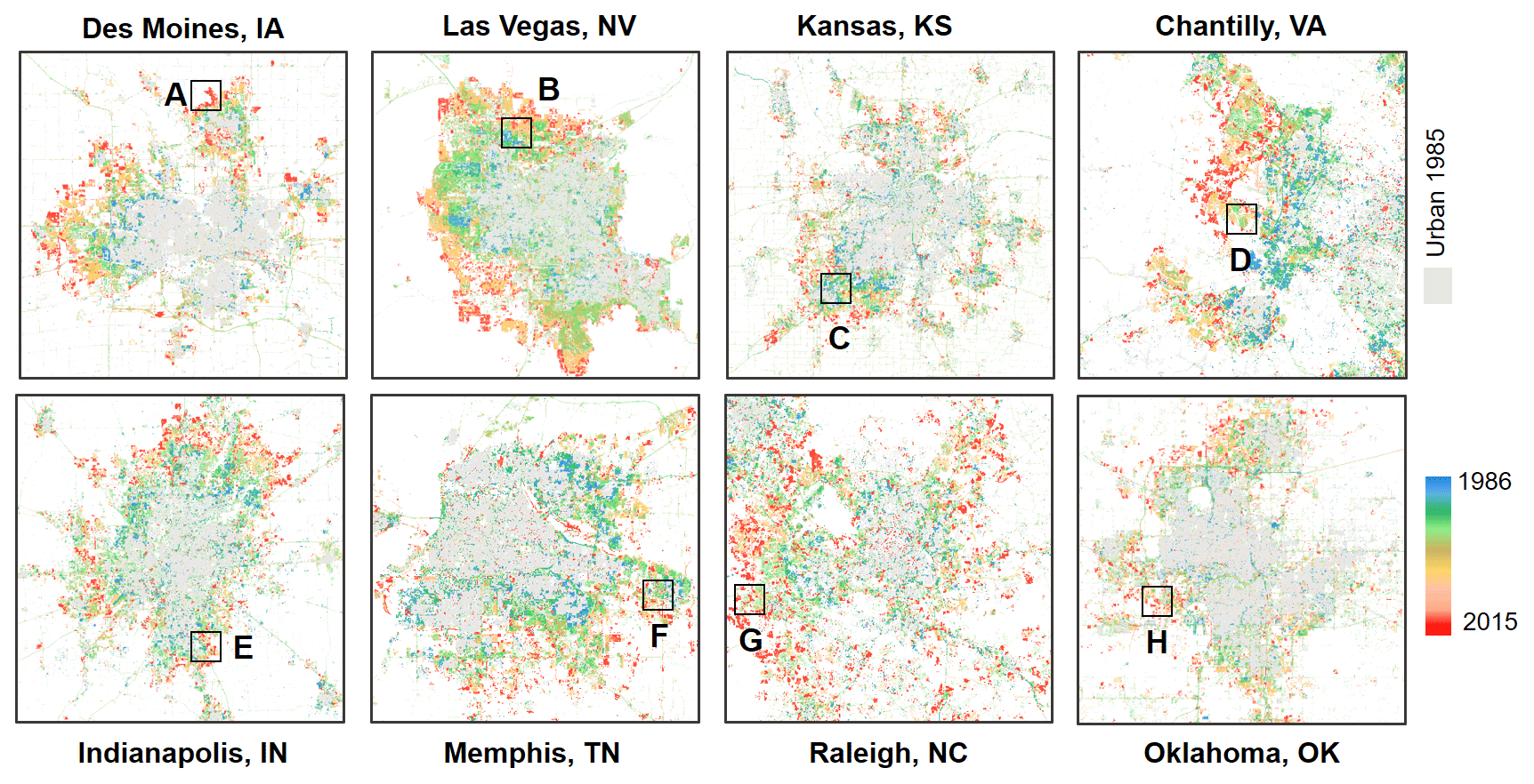
Figure 10Annual dynamics of urban extent in eight selected US cities over the past three decades. The black frames are regions in Fig. 11 for further comparison with Landsat images.
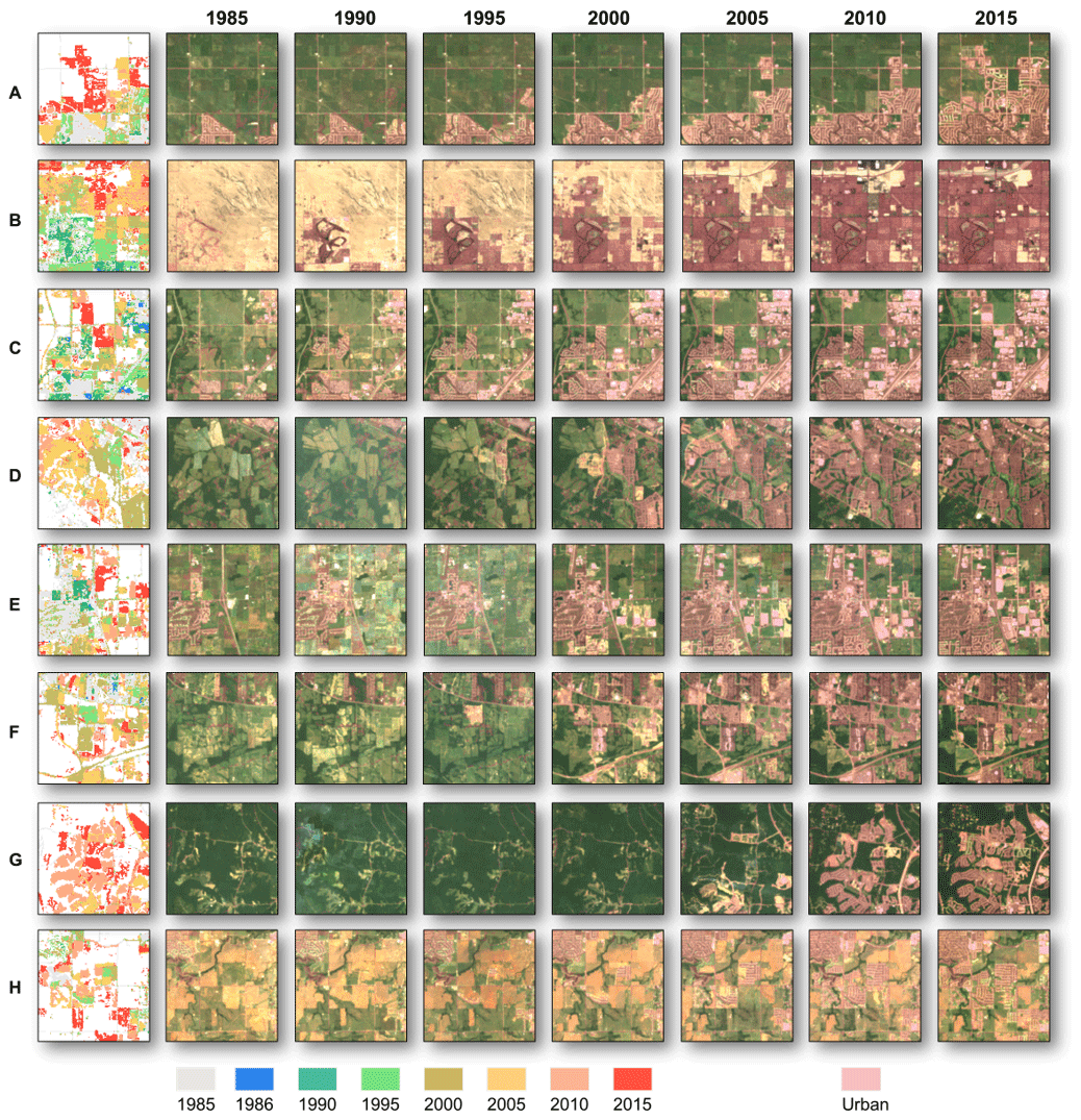
Figure 11Comparison of annual urban dynamics with Landsat images. The geographic location of each region (A–H) corresponds to the black frames in Fig. 10. The spatial extent of each region is 25 km2.
4.4.2 Classification of urbanized areas in periods B1 and F1
The CVA-based approach performs well for classifying urbanized areas, according to the accuracy assessment using samples randomly generated on both nonurban and urbanized areas during the periods B1 (1985–1992) and F1 (2011–2015) (Table 1). Validation samples for period B1 were randomly collected from persistent urban areas since 1985 and urbanized areas during 1985–1992. For the period F1, samples were generated based on nonurban areas and urbanized areas during 2011–2015, within the VIIRS-derived potential urban boundary (Fig. S8). The manual interpretation is based on the time series of Landsat and high-resolution Google Earth images in the two periods. The overall accuracies of classified urbanized areas for periods B1 and F1 are 96 % and 88 %, respectively (Table 1). The higher accuracy in the period B1 compared with the period F1 is because the validation samples in this period are within the possible urban extent of 1992 from the NLCD. Also, the misclassified urbanized areas in the period F1 are mainly caused by the confusion between bared land (e.g., rocks, or dry soil) and an urban area with similar spectral features (Mertes et al., 2015).
Table 1Accuracy assessment of classified urbanized areas for periods B1 and F1.

4.4.3 Uncertainties of annual urban extent data
There are several sources of uncertainties in our annual urban extent data. The first is the classification error in the NLCD, despite this being the most reliable database in the US with a fine resolution and multiple periods (Homer et al., 2015). On the one hand, the detected change information is incorrect in the misclassified urbanized pixels from NLCD. On the other hand, for those urbanized pixels, but not identified in NLCD, their change information is not captured in our result. However, the overall accuracy of land cover classification in NLCD is about 85 %–90 % (Wickham et al., 2017), and the accuracy of urban land cover is even higher (i.e., larger than 95 % in selected examples of US) (Li et al., 2018). Moreover, the CVA-based approach can be implemented to improve the urban extent maps of NLCD as change magnitudes of those pseudo-urban pixels in the NLCD are notably lower than changes caused by urban sprawl. In addition, the omitted urbanized pixels in the NLCD can be potentially captured using the CVA-based approach. The second is the classification error in mapped urbanized areas in the beginning and ending years. Uncertainties caused by spectral similarities between urban and bared lands could still exist in our results (Table 1), although we have used different constraints (e.g., change vector, classification results, and NTL) to mitigate such uncertainties. More advanced classification algorithms and additional information such as thermal features could be helpful for improving our algorithm in monitoring urban dynamics.
The generated data of annual urban dynamics are available at https://doi.org/10.6084/m9.figshare.8190920.v2 (Li et al., 2019c). The dataset is organized by state (total 49) in the conterminous US. The location of US states can be found in the figure “US_State.jpg”. Full names and abbreviations of US states are provided in the file “US_StateList.xls”. The data are in GeoTIFF, with the georeferenced information embedded. Each file was projected to the Albers equal-area conic projection, with a spatial resolution of 30 m. The legend of the GeoTIFF file can be found in the figure “Legend.jpg”. The lookup table between pixel values (1–31) and urbanized years (1985–2015) can be found in the file “Year_Code_Loopup.csv”. The National Land Cover Database was retrieved from the US Geological Survey at https://www.mrlc.gov/data (US Geological Survey, 2019), and the VIIRS nighttime light data were downloaded from the National Oceanic and Atmospheric Administration at https://ngdc.noaa.gov/eog/download.html (NOAA, 2019).
In this study, we mapped annual urban extents in the conterminous US by developing an efficient framework on the GEE platform using long-term Landsat observations. First, aided by the NLCD, we temporally grouped the entire temporal span into four periods (i.e., B1: 1985–1992; B2: 1992–2001, B3: 2001–2011; and F1: 2011–2015). Then, we derived the urbanized years and change magnitudes measured by indicators of NDVI, MNDWI, and SWIR at the pixel level, using a temporal segmentation approach in each period. After that, we classified urbanized areas at the cluster level in the beginning (1985) and the ending (2015) years through the implementation of a CVA-based approach. Considering the spatially explicit urban sprawl over large areas, we developed a unique hierarchical strategy to apply the CVA-based approach at the national level. Finally, the mapped urban dynamics in these four periods were combined as a complete dataset of 30-year dynamics of urban extent in the conterminous US.
The proposed mapping framework with the unique hierarchical strategy achieves a good performance in mapping annual dynamics of urban extent at a fine spatial resolution at the national level. The overall accuracies of detected urbanized years for the periods B1, B2, and B3 are 89 %, 83 %, and 88 %, respectively, with a 1-year tolerance strategy. Meanwhile, the CVA-based approach on the output from temporal segmentation can classify urbanized areas well, with overall accuracies of 96 % and 88 % for periods B1 and F1, respectively. Also, the implementation of the CVA-based approach using the proposed hierarchical strategy can capture the heterogeneity of urban growth over different regions, periods, and urban sizes, which helps to build a reliable dataset of urban dynamics.
There is a notable difference in the growth rates and patterns of annual urban areas across states in the US over the past three decades. The total increment of urban areas is about 31 000 km2, which accounts for around 20 % of the urban area in 1985. The long-term growth of urban areas is not linear over the years. The results suggest there is an increasing trend of urban area growth in the early years of 2001–2011 and then a decreasing trend in the latter years. Using the annual time series data of urban areas, we observed a plateaued growth pattern of urban areas in most coastal states and an accelerated growth pattern in the Midwestern US. Besides, the cropland is the most predominant source of increased urban areas, accounting for 46 % of the total urbanized areas during 1992–2015.
This study provides a successful application of mapping annual urban extent at the national scale through the combination of existing good-quality NLCD urban extent maps, long-term Landsat time series data, and the GEE cloud-based platform. The proposed approach can be transferred to other regions with similar multitemporal land cover datasets to the NLCD, for updating existing land cover datasets with a higher temporal resolution. This study opens a new avenue to use all available Landsat observations for mapping annual urban extent at the national level compared with previous studies using the supervised classification or postprocessing (Schneider et al., 2010; Li et al., 2015; Liu and Cai, 2012). Moreover, the derived change information from the temporal segmentation using annual observations is more reliable compared with the research using a pair of Landsat images in 2 years (Yu et al., 2016). However, this approach may introduce uncertainties if the composited annual time series Landsat observations fluctuate too much, especially when this fluctuation is larger than the change induced by urbanization.
The supplement related to this article is available online at: https://doi.org/10.5194/essd-12-357-2020-supplement.
YZ and XL designed the research. XL and YZ implemented the research and wrote the paper. ZZ and WC revised the paper.
The authors declare that they have no conflict of interest.
This research was funded in part by the US Department of Agriculture (USDA) and Iowa State University. We would like to thank the organizations that shared their datasets for use in this study.
This research has been supported by the USDA Natural Resources Conservation Service (grant no. 68-7482-17-009).
This paper was edited by Kirsten Elger and reviewed by two anonymous referees.
Alberti, M., Correa, C., Marzluff, J. M., Hendry, A. P., Palkovacs, E. P., Gotanda, K. M., Hunt, V. M., Apgar, T. M., and Zhou, Y.: Global urban signatures of phenotypic change in animal and plant populations, P. Natl. Acad. Sci. USA, 114, 8951–8956, https://doi.org/10.1073/pnas.1606034114, 2017.
Andersson, E. and Colding, J.: Understanding how built urban form influences biodiversity, Urban For. Urban Green., 13, 221–226, 2014.
Cao, W., Zhou, Y., Li, R., and Li, X.: Mapping changes in coastlines and tidal flats in developing islands using the full time series of Landsat images, Remote Sens. Environ., 239, 111665, https://doi.org/10.1016/j.rse.2020.111665, 2020.
Chen, J., Chen, J., Liao, A., Cao, X., Chen, L., Chen, X., He, C., Han, G., Peng, S., Lu, M., Zhang, W., Tong, X., and Mills, J.: Global land cover mapping at 30 m resolution: A POK-based operational approach, ISPRS J. Photogramm. Remote Sens., 103, 7–27, https://doi.org/10.1016/j.isprsjprs.2014.09.002, 2015.
Chen, Y., Li, X., Zheng, Y., Guan, Y., and Liu, X.: Estimating the relationship between urban forms and energy consumption: A case study in the Pearl River Delta, 2005–2008, Landscape Urban Plan, 102, 33–42, 2011.
Fan, C., Tian, L., Zhou, L., Hou, D., Song, Y., Qiao, X., and Li, J.: Examining the impacts of urban form on air pollutant emissions: Evidence from China, J. Environ. Manage., 212, 405–414, https://doi.org/10.1016/j.jenvman.2018.02.001, 2018.
Fry, J., Coan, M., Homer, C., Meyer, D., and Wickham, J.: Completion of the National Land Cover Database (NLCD) 1992–2001 land cover change retrofit product, Reston, VA, Report 2008-1379, 2009.
Gong, P., Liang, S., Carlton, E. J., Jiang, Q., Wu, J., Wang, L., and Remais, J. V.: Urbanisation and health in China, Lancet, 379, 843–852, https://doi.org/10.1016/S0140-6736(11)61878-3, 2012.
Gong, P., Wang, J., Yu, L., Zhao, Y., Zhao, Y., Liang, L., Niu, Z., Huang, X., Fu, H., Liu, S., Li, C., Li, X., Fu, W., Liu, C., Xu, Y., Wang, X., Cheng, Q., Hu, L., Yao, W., Zhang, H., Zhu, P., Zhao, Z., Zhang, H., Zheng, Y., Ji, L., Zhang, Y., Chen, H., Yan, A., Guo, J., Yu, L., Wang, L., Liu, X., Shi, T., Zhu, M., Chen, Y., Yang, G., Tang, P., Xu, B., Giri, C., Clinton, N., Zhu, Z., Chen, J., and Chen, J.: Finer resolution observation and monitoring of global land cover: first mapping results with Landsat TM and ETM+ data, Int. J. Remote Sens., 34, 2607–2654, https://doi.org/10.1080/01431161.2012.748992, 2013.
Gong, P., Li, X., and Zhang, W.: 40-year (1978–2017) human settlement changes in China reflected by impervious surfaces from satellite remote sensing, Sci. Bull., 64, 756–763, https://doi.org/10.1016/j.scib.2019.04.024, 2019.
Gong, P., Li, X., Wang, J., Bai, Y., Chen, B., Hu, T., Liu, X., Xu, B., Yang, J., Zhang, W., and Zhou, Y.: Annual maps of global artificial impervious areas (GAIA) between 1985 and 2018, Remote Sens. Environ., 236, 111510, https://doi.org/10.1016/j.rse.2019.111510, 2020.
Gorelick, N., Hancher, M., Dixon, M., Ilyushchenko, S., Thau, D., and Moore, R.: Google Earth Engine: Planetary-scale geospatial analysis for everyone, Remote Sens. Environ., 202, 18–27, https://doi.org/10.1016/j.rse.2017.06.031, 2017.
Güneralp, B., Zhou, Y., Ürge-Vorsatz, D., Gupta, M., Yu, S., Patel, P. L., Fragkias, M., Li, X., and Seto, K. C.: Global scenarios of urban density and its impacts on building energy use through 2050, P. Natl. Acad. Sci. USA, 114, 8945–8950, https://doi.org/10.1073/pnas.1606035114, 2017.
Homer, C. G., Dewitz, J. A., Yang, L., Jin, S., Danielson, P., Xian, G., Coulston, J., Herold, N. D., Wickham, J., and Megown, K.: Completion of the 2011 National Land Cover Database for the conterminous United States-Representing a decade of land cover change information, Photogramm. Eng. Remote Sens., 81, 345–354, 2015.
Huang, C., Goward, S. N., Masek, J. G., Thomas, N., Zhu, Z., and Vogelmann, J. E.: An automated approach for reconstructing recent forest disturbance history using dense Landsat time series stacks, Remote Sens. Environ., 114, 183–198, https://doi.org/10.1016/j.rse.2009.08.017, 2010.
Irwin, E. G. and Bockstael, N. E.: The evolution of urban sprawl: Evidence of spatial heterogeneity and increasing land fragmentation, P. Natl. Acad. Sci. USA, 104, 20672–20677, https://doi.org/10.1073/pnas.0705527105, 2007.
Kennedy, R. E., Yang, Z., and Cohen, W. B.: Detecting trends in forest disturbance and recovery using yearly Landsat time series: 1. LandTrendr – Temporal segmentation algorithms, Remote Sens. Environ., 114, 2897–2910, https://doi.org/10.1016/j.rse.2010.07.008, 2010.
Li, X. and Gong, P.: Urban growth models: progress and perspective, Sci. Bull., 61, 1637–1650, https://doi.org/10.1007/s11434-016-1111-1, 2016a.
Li, X. and Gong, P.: An “exclusion-inclusion” framework for extracting human settlements in rapidly developing regions of China from Landsat images, Remote Sens. Environ., 186, 286–296, https://doi.org/10.1016/j.rse.2016.08.029, 2016b.
Li, X. and Zhou, Y.: Urban mapping using DMSP/OLS stable night-time light: a review, Int. J. Remote Sens., 38, 1–17, https://doi.org/10.1080/01431161.2016.1274451, 2017.
Li, X., Liu, X., and Yu, L.: A systematic sensitivity analysis of constrained cellular automata model for urban growth simulation based on different transition rules, Int. J. Geogr. Inf. Sci., 28, 1317–1335, https://doi.org/10.1080/13658816.2014.883079, 2014.
Li, X., Gong, P., and Liang, L.: A 30-year (1984–2013) record of annual urban dynamics of Beijing City derived from Landsat data, Remote Sens. Environ., 166, 78–90, https://doi.org/10.1016/j.rse.2015.06.007, 2015.
Li, X., Zhou, Y., Asrar, G. R., Mao, J., Li, X., and Li, W.: Response of vegetation phenology to urbanization in the conterminous United States, Glob. Change Biol., 23, 2818–2830, https://doi.org/10.1111/gcb.13562, 2017.
Li, X., Zhou, Y., Zhu, Z., Liang, L., Yu, B., and Cao, w.: Mapping annual urban dynamics (1985–2015) using time series of Landsat data, Remote Sens. Environ., 216, 674–683, 2018.
Li, X., Zhou, Y., Eom, J., Yu, S., and Asrar, G. R.: Projecting global urban area growth through 2100 based on historical time-series data and future Shared Socioeconomic Pathways, Earth's Future, 7, 351–362, https://doi.org/10.1029/2019EF001152, 2019a.
Li, X., Zhou, Y., Meng, L., Asrar, G. R., Lu, C., and Wu, Q.: A dataset of 30 m annual vegetation phenology indicators (1985–2015) in urban areas of the conterminous United States, Earth Syst. Sci. Data, 11, 881–894, https://doi.org/10.5194/essd-11-881-2019, 2019b.
Li, X., Zhou, Y., Zhu, Z., and Cao, W.: A national dataset of annual urban extent (1985–2015) in the conterminous United States using Landsat time series data, figshare, Dataset, https://doi.org/10.6084/m9.figshare.8190920.v2, 2019c.
Liu, D. and Cai, S.: A Spatial-Temporal Modeling Approach to Reconstructing Land-Cover Change Trajectories from Multi-temporal Satellite Imagery, Ann. Assoc. Am. Geogr., 102, 1329–1347, https://doi.org/10.1080/00045608.2011.596357, 2012.
Liu, X., Hu, G., Chen, Y., Li, X., Xu, X., Li, S., Pei, F., and Wang, S.: High-resolution multi-temporal mapping of global urban land using Landsat images based on the Google Earth Engine Platform, Remote Sens. Environ., 209, 227–239, https://doi.org/10.1016/j.rse.2018.02.055, 2018.
Lu, D. and Weng, Q.: Spectral mixture analysis of the urban landscape in Indianapolis with Landsat ETM+ imagery, Photogramm. Eng. Rem. S., 70, 1053–1062, 2004.
Luber, G., Knowlton, K., Balbus, J., Frumkin, H., Hayden, M., Hess, J., McGeehin, M., Sheats, N., Backer, L., Beard, C. B., Ebi, K. L., Maibach, E., Ostfeld, R. S., Wiedinmyer, C., Zielinski-Gutiérrez, E., and Ziska, L.: chap. 9: Human Health, in: Climate Change Impacts in the United States: The Third National Climate Assessment, edited by: Melillo, J. M., Richmond, T. C., and Yohe, G. W., US Global Change Research Program, 220–256, 2014.
Masek, J. G., Vermote, E. F., Saleous, N. E., Wolfe, R., Hall, F. G., Huemmrich, K. F., Gao, F., Kutler, J., and Lim, T.-K.: A Landsat surface reflectance dataset for North America, 1990–2000, IEEE Geosci. Remote Sens. Lett., 3, 68–72, 2006.
Mertes, C. M., Schneider, A., Sulla-Menashe, D., Tatem, A. J., and Tan, B.: Detecting change in urban areas at continental scales with MODIS data, Remote Sens. Environ., 158, 331–347, https://doi.org/10.1016/j.rse.2014.09.023, 2015.
Morisette, J. T. and Khorram, S.: Accuracy assessment curves for satellite-based change detection, Photogramm. Eng. Rem. S., 66, 875–880, 2000.
National Oceanic and Atmospheric Administration: The VIIRS nighttime light data, available at: https://ngdc.noaa.gov/eog/download.html, last access: 20 April 2019.
Peng, S., Piao, S., Ciais, P., Friedlingstein, P., Ottle, C., Bréon, F.-M., Nan, H., Zhou, L., and Myneni, R. B.: Surface Urban Heat Island Across 419 Global Big Cities, Environ. Sci. Technol., 46, 696–703, https://doi.org/10.1021/es2030438, 2012.
Rodriguez, R. S., Ürge-Vorsatz, D., and Barau, A. S.: Sustainable Development Goals and climate change adaptation in cities, Nat. Clim. Change, 8, 181–183, 2018.
Roy, D. P., Kovalskyy, V., Zhang, H. K., Vermote, E. F., Yan, L., Kumar, S. S., and Egorov, A.: Characterization of Landsat-7 to Landsat-8 reflective wavelength and normalized difference vegetation index continuity, Remote Sens. Environ., 185, 57–70, https://doi.org/10.1016/j.rse.2015.12.024, 2016.
Santé, I., García, A. M., Miranda, D., and Crecente, R.: Cellular automata models for the simulation of real-world urban processes: A review and analysis, Landscape Urban Plan., 96, 108–122, https://doi.org/10.1016/j.landurbplan.2010.03.001, 2010.
Schneider, A., Friedl, M. A., and Potere, D.: Mapping global urban areas using MODIS 500-m data: New methods and datasets based on 'urban ecoregions', Remote Sens. Environ., 114, 1733–1746, https://doi.org/10.1016/j.rse.2010.03.003, 2010.
Seto, K. C., Woodcock, C. E., Song, C., Huang, X., Lu, J., and Kaufmann, R. K.: Monitoring land-use change in the Pearl River Delta using Landsat TM, Int. J. Remote Sens., 23, 1985–2004, https://doi.org/10.1080/01431160110075532, 2002.
Sexton, J. O., Song, X.-P., Huang, C., Channan, S., Baker, M. E., and Townshend, J. R.: Urban growth of the Washington, DC, Baltimore, MD metropolitan region from 1984 to 2010 by annual, Landsat-based estimates of impervious cover, Remote Sens. Environ., 129, 42–53, https://doi.org/10.1016/j.rse.2012.10.025, 2013.
Shi, L., Ling, F., Ge, Y., Foody, G., Li, X., Wang, L., Zhang, Y., and Du, Y.: Impervious Surface Change Mapping with an Uncertainty-Based Spatial-Temporal Consistency Model: A Case Study in Wuhan City Using Landsat Time-Series Datasets from 1987 to 2016, Remote Sens., 9, 1148, https://doi.org/10.3390/rs9111148, 2017.
Solecki, W., Seto, K. C., and Marcotullio, P. J.: It's Time for an Urbanization Science, Environment: Science and Policy for Sustainable Development, Environment: Science and Policy for Sustainable Development, 55, 12–17, https://doi.org/10.1080/00139157.2013.748387, 2013.
Song, X.-P., Sexton, J. O., Huang, C., Channan, S., and Townshend, J. R.: Characterizing the magnitude, timing and duration of urban growth from time series of Landsat-based estimates of impervious cover, Remote Sens. Environ., 175, 1–13, https://doi.org/10.1016/j.rse.2015.12.027, 2016.
United Nations: World Urbanization Prospects: The 2018 Revision (ST/ESA/SER.A/420), New York, United Nations, 2019.
US Geological Survey: The National Land Cover Database, available at: https://www.mrlc.gov/data, last access: 20 April 2019.
Weng, Q.: Remote sensing of impervious surfaces in the urban areas: Requirements, methods, and trends, Remote Sens. Environ., 117, 34–49, https://doi.org/10.1016/j.rse.2011.02.030, 2012.
Wickham, J., Stehman, S. V., Gass, L., Dewitz, J. A., Sorenson, D. G., Granneman, B. J., Poss, R. V., and Baer, L. A.: Thematic accuracy assessment of the 2011 National Land Cover Database (NLCD), Remote Sens. Environ., 191, 328–341, https://doi.org/10.1016/j.rse.2016.12.026, 2017.
Wickham, J. D., Stehman, S. V., Fry, J. A., Smith, J. H., and Homer, C. G.: Thematic accuracy of the NLCD 2001 land cover for the conterminous United States, Remote Sens. Environ., 114, 1286–1296, https://doi.org/10.1016/j.rse.2010.01.018, 2010.
Xian, G., Homer, C., and Fry, J.: Updating the 2001 National Land Cover Database land cover classification to 2006 by using Landsat imagery change detection methods, Remote Sens. Environ., 113, 1133–1147, https://doi.org/10.1016/j.rse.2009.02.004, 2009.
Xie, Y. and Weng, Q.: Updating urban extents with nighttime light imagery by using an object-based thresholding method, Remote Sens. Environ., 187, 1–13, https://doi.org/10.1016/j.rse.2016.10.002, 2016.
Xie, Y. and Weng, Q.: Spatiotemporally enhancing time-series DMSP/OLS nighttime light imagery for assessing large-scale urban dynamics, ISPRS J. Photogramm. Remote Sens., 128, 1–15, 2017.
Yu, W., Zhou, W., Qian, Y., and Yan, J.: A new approach for land cover classification and change analysis: Integrating backdating and an object-based method, Remote Sens. Environ., 177, 37–47, https://doi.org/10.1016/j.rse.2016.02.030, 2016.
Zhang, Z., Wang, X., Zhao, X., Liu, B., Yi, L., Zuo, L., Wen, Q., Liu, F., Xu, J., and Hu, S.: A 2010 update of National Land Use/Cover Database of China at 1:100 000 scale using medium spatial resolution satellite images, Remote Sens. Environ., 149, 142–154, https://doi.org/10.1016/j.rse.2014.04.004, 2014.
Zhou, Y., Clarke, L., Eom, J., Kyle, P., Patel, P., Kim, S. H., Dirks, J., Jensen, E., Liu, Y., Rice, J., Schmidt, L., and Seiple, T.: Modeling the effect of climate change on U.S. state-level buildings energy demands in an integrated assessment framework, Appl. Energ., 113, 1077–1088, https://doi.org/10.1016/j.apenergy.2013.08.034, 2014.
Zhou, Y., Smith, S. J., Zhao, K., Imhoff, M., Thomson, A., Bond-Lamberty, B., Asrar, G. R., Zhang, X., He, C., and Elvidge, C. D.: A global map of urban extent from nightlights, Environ. Res. Lett., 10, 1–11, https://doi.org/10.1088/1748-9326/10/5/054011, 2015.
Zhou, Y., Li, X., Asrar, G. R., Smith, S. J., and Imhoff, M.: A global record of annual urban dynamics (1992–2013) from nighttime lights, Remote Sens. Environ., 219, 206–220, 2018.