the Creative Commons Attribution 4.0 License.
the Creative Commons Attribution 4.0 License.
 | 23 Mar 2020
Soil moisture and matric potential – an open field comparison of sensor systems
Conrad Jackisch
Kai Germer
Thomas Graeff
Ines Andrä
Katrin Schulz
Marcus Schiedung
Jaqueline Haller-Jans
Jonas Schneider
Julia Jaquemotte
Philipp Helmer
Leander Lotz
Andreas Bauer
Irene Hahn
Martin Šanda
Monika Kumpan
Johann Dorner
Gerrit de Rooij
Stefan Wessel-Bothe
Lorenz Kottmann
Siegfried Schittenhelm
Wolfgang Durner
Soil water content and matric potential are central hydrological state variables. A large variety of automated probes and sensor systems for state monitoring exist and are frequently applied. Most applications solely rely on the calibration by the manufacturers. Until now, there has been no commonly agreed-upon calibration procedure. Moreover, several opinions about the capabilities and reliabilities of specific sensing methods or sensor systems exist and compete.
A consortium of several institutions conducted a comparison study of currently available sensor systems for soil water content and matric potential under field conditions. All probes were installed at 0.2 m b.s. (metres below surface), following best-practice procedures. We present the set-up and the recorded data of 58 probes of 15 different systems measuring soil moisture and 50 further probes of 14 different systems for matric potential. We briefly discuss the limited coherence of the measurements in a cross-correlation analysis.
The measuring campaign was conducted during the growing period of 2016. The monitoring data, results from pedophysical analyses of the soil and laboratory reference measurements for calibration are published in Jackisch et al. (2018, https://doi.org/10.1594/PANGAEA.892319).


Soil water content is defined as the volumetric proportion of water in the multiphase bulk soil. Since the proposition of soil moisture determination based on relative electrical permittivity of the bulk soil in the 1970s (presumably starting with Davis et al., 1966; Geiger and Williams, 1972; Chudobiak et al., 1979) many commercially available systems have been developed. They can be roughly grouped into time-domain reflectometry (TDR), mostly impedance-based determination of the capacitance and time-domain transmission (TDT) techniques, which all rely on the strong contrast of the relative electrical permittivity of water (80) with air (1) and minerals (3–5) in the bulk soil. However, the relative electrical permittivity is also influenced by temperature (Roth et al., 1990; Wraith and Or, 1999; Owen et al., 2002; Rosenbaum et al., 2011), soil texture (Ponizovsky et al., 1999) and organisation of thin water film layers (Wang and Schmugge, 1980). In addition, there is a frequency dependency of such measurements. While low measurement frequencies might be dominated by bulk electrical conductivity (Schwartz et al., 2013), also higher frequencies emphasise more or less the effects of solutes, clay surfaces and organic matter on the conductor and dielectric properties (Loewer et al., 2017).
In addition to the theoretical concerns, the sensing systems need to solve a series of technical issues, e.g. the sensor wiring and coupling; the facilitation of the signal propagation from the sensor into the soil; and stability of the measurements themselves to corrosion, shielding and temperature. Thus one has to be aware that the theoretically more appropriate TDR technology might not deliver more precise readings per se when technical issues obscure the actual measurement. Another common assumption relates to a large sensing volume being more favourable. However, neither effects of a change of the sensed soil volume with changing bulk permittivity nor the influence of the distribution of water within this volume can be usually specified.
Accompanying soil water content, matric potential is the second central hydrological state variable of soils. It is an integral over the macroscopic interfacial tension of the pore-scale menisci of all air–water–soil interfaces. It was introduced by Buckingham (1907) and Gardner and Widtsoe (1921) as capillary potential and combines the effects of soil water content, pore space characteristics and the respective configuration of the soil water in the pore space. Tensiometers have been used for over a century to directly measure the capillary tension (Or, 2001). Because the measurement is limited to the vaporisation point of water in the tensiometer against an atmospheric pressure at approximately 1000 hPa, polymer-based versions (van der Ploeg et al., 2010) and alternative sensing techniques measuring matric potential indirectly through water content detection in a porous ceramic material with known retention properties have been developed.
In order to identify conceptual limits and technological issues of currently available systems for measurement of soil water content and matric potential we conducted a comparison study under field conditions. For this, a large number of sensors were installed in a specifically homogenised and levelled agricultural field with loamy sandy soil. Vegetation effects were excluded by glyphosate treatment. The test was conducted from May to November 2016.
2.1 Site description and study layout
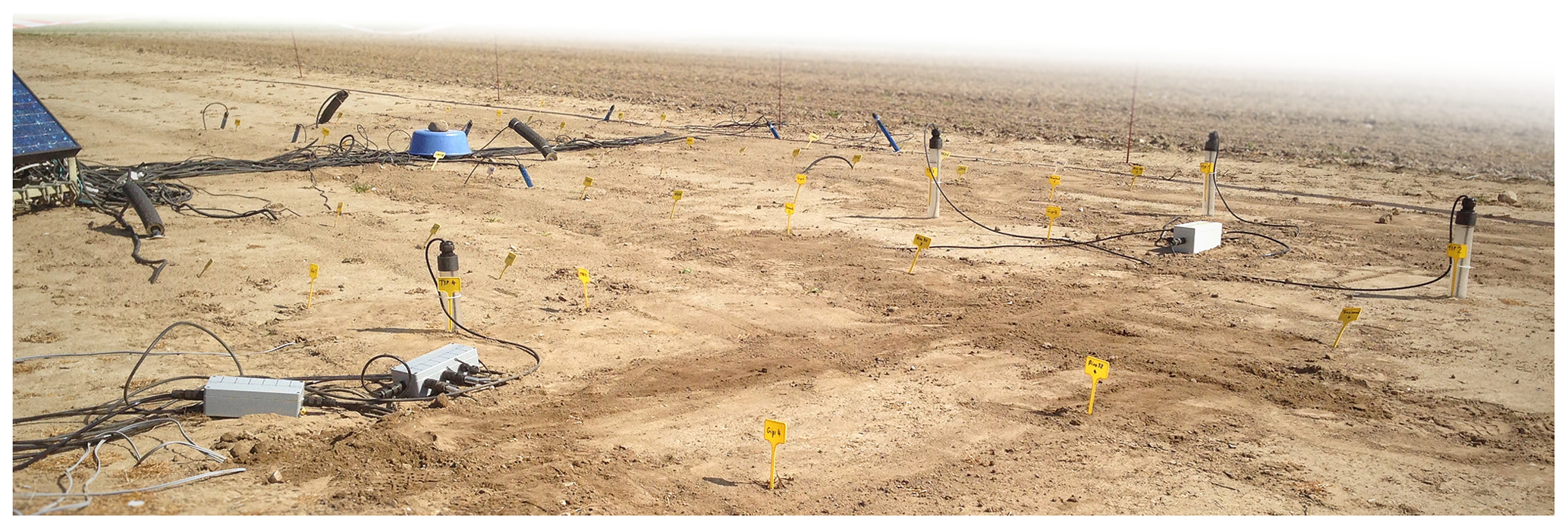
The study site is located on an agricultural test site of the Julius Kühn-Institut, Braunschweig, Germany (52.2964∘ N, 10.4361∘ E; Fig. 1). The site is characterised by loess and sand depositions over marls of the last glacial periods in a plain with very little relief. The soil is very homogeneous sandy loam with gravel content below 3 %. The plot was prepared by harrowing, ploughing and compacting. In order to keep the system as simple as possible, vegetation was suppressed by glyphosate application.

Figure 2Layout of the sensor comparison field site. Each grid cell covers 0.5 m×0.5 m. All sensors are placed at 0.2 m depth. Positions of soil samples marked with dots. Total covered area 14 m in east–west and 4 m in north–south extent.
The sensors were installed in a grid of 0.5 m distance (Fig. 2) at 0.2 m depth, following the best-practice recommendation of the manufacturers. The total covered area amounts to 14 m in the east–west and 4 m in the north–south extent. Whenever the probe design allowed (round shape with suitable diameter), insertion from the surface with minimal disturbance using an auger tilted by 45∘ was chosen. Alternatively, probes were positioned horizontally below undisturbed surface from a shallow access pit. Probes which included their access tubes were installed vertically. In order to avoid compaction of the surface by walking on it, plywood panes were temporally placed along the access paths during the fieldwork. Installation took place over several campaigns in April and May 2016. The field was exposed to natural weather conditions until 24 August 2016. After that date, a tunnel greenhouse was installed for protection against rain in order to reach lower matric potentials. Adverse effects of drainage from the tunnel near the edges of the tunnel appear to have occurred later in the year. The full dataset is included in the repository. However, we focus on the period until 24 August in this study.
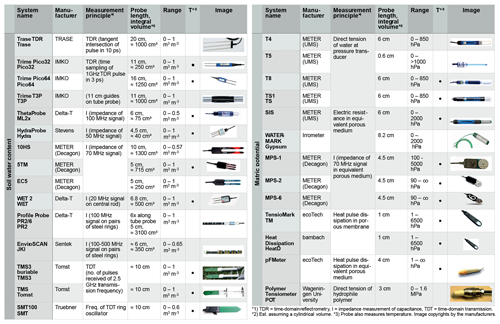
Table 1Employed sensor systems in the comparison study. All information according to the respective manufacturer.
2.2 Sensor systems
In total 58 probes of 15 different systems measuring soil moisture and 50 probes of 14 different systems for matric potential were used. Each sensor of a system has two to four replicates. An overview about the sensor systems is given in Table 1. All sensors are utilised with the manufacturer's calibration.
Soil moisture is measured based on electromagnetic estimates of the bulk soil relative permittivity, which is mostly controlled by water. For this, four systems use the TDR (time-domain reflectometry) method. They differ in the sampling and evaluation technique of the travel time of a pulse along the waveguides. While the Trase system evaluates the intersection of tangent lines of the incoming and reflected pulse voltages (Soilmoisture Equipment inc., 1996), the Trime systems perform time measurements at distinct voltage levels (Stacheder et al., 1997). Eight systems measure the capacitance of the bulk soil by impedance of oscillating pulses. They differ mostly in the applied frequency and geometry of the set-up. Two systems use a TDT (time-domain transmission) technique, which estimates the soil bulk permittivity by counting received pulses emitted at high frequency (Wild et al., 2019). One system extends the TDT technique by determining the oscillation frequency of a TDT system (Bogena et al., 2017).
Matric potential is measured either directly through a pressure transducer in tensiometers or through soil moisture measurements in an EPM (equivalent porous medium) with known soil water retention properties. For the EPM, two systems measure the electric resistance of a gypsum EPM, which is related to its moisture. Three systems use the impedance measurement described above. Three systems estimate the moisture by measuring the dissipation of a heat pulse in the EPM. One system uses a hydrophile polymer instead of water to extend the measurement range of the tensiometers (Bakker et al., 2007).
2.3 Pedophysical analyses
Eight undisturbed ring samples (250 mL) taken at 0.2 m depth near the probes (dots in Fig. 2) were analysed for soil water retention properties (HYPROP and WP4C, METER Group). The first batch of samples was taken during the sensor installation on 21 April 2016. The three samples were taken at the end of the experiment on 6 December 2016. These were also analysed for saturated hydraulic conductivity (KSAT, METER Group), texture (sedimentation method after DIN ISO 11277), organic matter (ignition loss after DIN EN 13039) and pH (in a suspension in 0.01 mol L−1 CaCl2 using a WTW pH electrode after DIN ISO 10390).
2.4 Laboratory reference
As a reference measurement intended for a posteriori calibration, an undisturbed, cylindrical soil monolith of 15.7 L (0.3 m height, 0.26 m diameter) was sampled at 0.05–0.35 m depth and equipped with six soil moisture sensors of three of the employed systems (Pico32, 10HS and 5TM). The probes were selected based on the plausibility of their records in the field, their size for the laboratory installation and availability. We installed the probes vertically in the same depth, referenced to the centre of the probes. The monolith was initially saturated and exposed to free evaporation for 3 weeks and set up on a weighing scale in the lab. Referenced against the dry weight of the whole set-up, this delivers time series of gravimetric soil water content plus the readings from six sensors. In order to avoid overly strong internal soil moisture gradients due to evaporation at the surface, the sample was periodically covered.
The data and some exemplary analysis are hosted in the PANGAEA repository (Jackisch et al., 2018, https://doi.org/10.1594/PANGAEA.892319).
3.1 Pedophysical data
The pedophysical data are given in pedophysical_data.xlsx as a table of analyses of eight undisturbed ring samples. Sample nos. 1–5 were taken on 21 April 2016 during the first sensor installation campaign. Sample nos. 6–8 were taken on 6 December 2016 during the first sensor removals. Bulk density (BD) was determined by referring the dry weight of the bulk soil after oven drying at 105 ∘C for 3 d to the sample volume of 250 mL. Porosity was estimated based on the soil water content at full saturation at the onset of the retention curve measurements using the free evaporation method of the HYPROP apparatus referring the total weight under saturated conditions to the dry weight. Over the course of the measurement of the HYPROP, tensions in the sample are referred to the total weight, resulting in the retention curve from pF 0 to pF 2.5 (with pF as decadic logarithm of the matric potential in hPa). To measure pairs of total weight and matric potential, the samples were processed in a WP4C chilled-mirror potentiometer. An overview is given in Fig. 3. The resulting measurements were processed in the HYPROP-FIT software (version 3.5.1, METER Group; original files given as hyprop.zip, and exported derivatives are stored in vG_JKI_params.xlsx, ku_obs.xlsx, retention_obs.xlsx and hyprop.xlsx) for fitting the original van Genuchten pedotransfer model (Van Genuchten, 1980) with the free m parameter. The resulting parameters for saturated soil water content (θsat; m3 m−3), residual soil water content (θres; m3 m−3), α (m−1), n, m and diffusive-flow-estimated saturated hydraulic conductivity (; m s−1) are reported for each sample.
Figure 3 presents the van Genuchten parameters fitted to all retention measurements. Not surprisingly, the greatest differences relate to a spread in porosity. However given the few exceptions with tensions below pF 2 (100 hPa) in the recorded time series (Fig. 4c), the very strong coherence of the retention curves at higher tensions corroborates the high homogeneity at the site.
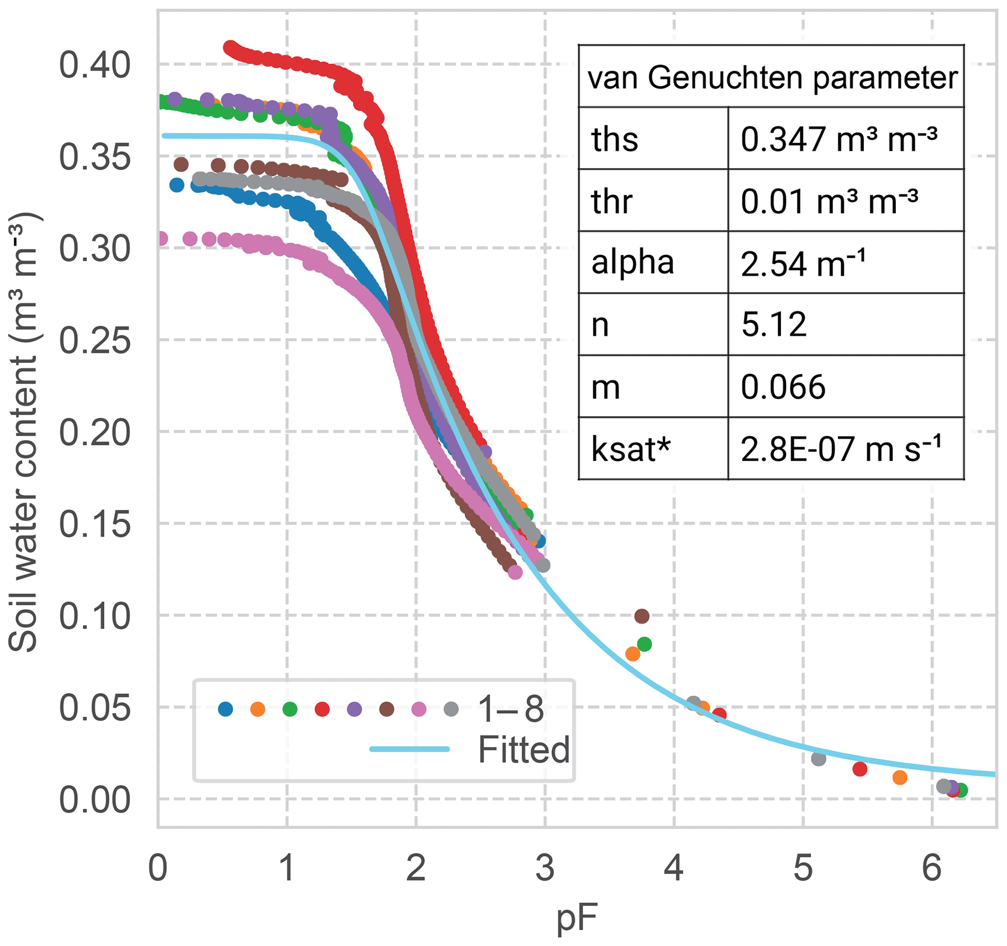
Figure 3Soil water retention data from eight 250 mL ring samples analysed in HYPROP and WP4C apparatus. Fitted van Genuchten model with free m parameter and diffusive hydraulic conductivity estimate.
3.2 Monitoring data
The monitoring data of all sensors are compiled in the files Theta20.xslx, Psi20.xlsx and T20.xlsx, holding volumetric soil water content (m3 m−3), matric potential (hPa) and soil temperature (∘C) respectively. The data of all individual sensors were merged into the common tables, aggregated to 30 min averages. The data were filtered for obvious measurement errors outside of the physically possible ranges. Initial inconsistencies of the time stamps from different loggers were removed by time-shift correction based on an analysis of the phase coherence of the diurnal temperature signal.
Meteorological reference is reported from the German Weather Service (DWD) Station 662, Braunschweig, through their Climate Data Centre (ftp://ftp-cdc.dwd.de/pub/CDC//observations_germany/climate/hourly, last access: 14 August 2018) referring to the station number. In addition, records of a weather station 100 m to the east of the plot is reported in meteo_jki.xlsx. It holds half-hourly records of solar radiation (W m−2), wind direction (∘), wind speed (m s−1), precipitation (mm per 0.5 h), air temperature (∘C) and relative air humidity (%). In addition calculated values for the dew point (∘C) and cumulative precipitation (mm) are given.
The measurements of volumetric soil water content and matric potential exhibit plausible dynamics in general. The sensors react to events and recover their ranks later on (Fig. 4). However, the different sensor classes deviate substantially with regard to their absolute values, to the intensity of the reaction to events, and to the existence and amplitude of diurnal cycles.
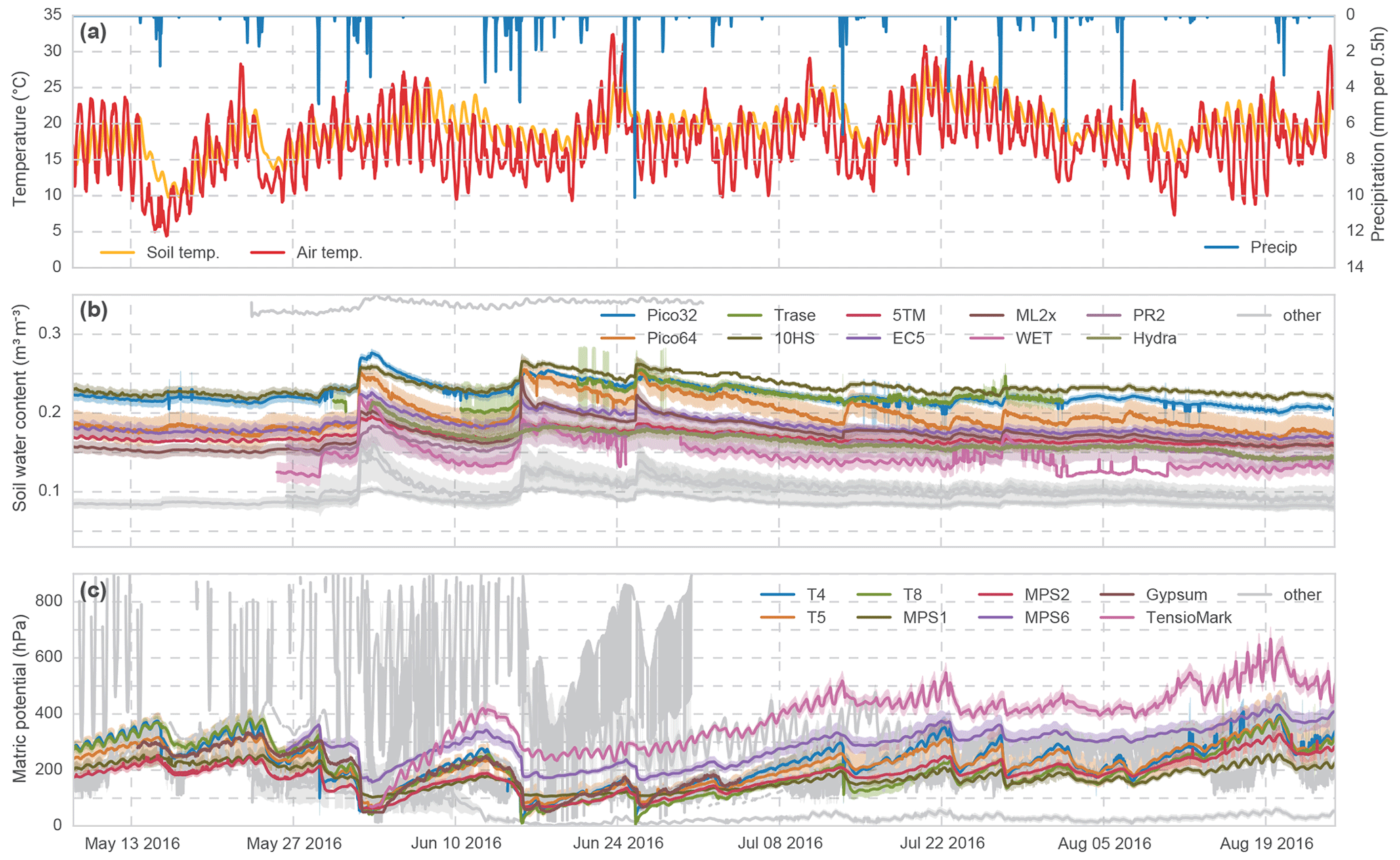
Figure 4(a) Meteorological forcing (DWD station 662), (b) volumetric soil water content dynamics and (c) matric potential; 30 min median of all sensors of a system as solid line, and variance is shaded. Sensor systems with non-plausible oscillations and value ranges are given as “other”.
3.3 Laboratory reference
Between 23 February and 21 March 2017, an undisturbed soil monolith was transferred to the laboratory, initially saturated and later left for drying. The monitored gravimetric soil water content and the readings from the installed sensors (all m3 m−3; 10 min means) are given in file lab_mono.xlsx. The gravimetric and sensed soil water content are not all linearly related. Interestingly, the capacitative sensors (5TM and 10HS) provide a better linear fit, although they deviated more strongly from the absolute values, while the TDR sensors present a non-linear relation (Fig. 5). In accordance with our records in the field experiment, the sensors of one system are highly congruent compared to larger differences between the systems. Also the ranking with the is the same. Moreover, the capacitive sensors show reoccurring shifts of the measurements over time, which coincide with the repeated coverage of the sample with an aluminium lid. These shifts resulted from changed configurations of the “capacitor”, consisting of the sample in a stainless-steel ring and a metal lid. From a point of view of measurement principles this application flaw should be considered in future calibration approaches, omitting effects of electrical currents through the sampling material.

Figure 5Soil water content in undisturbed monolith as laboratory reference. Gravimetric reference vs. sensor values of the three systems (colours) with one replicate each (shading).
4.1 Time series cross correlation
Most systems recorded plausible data, which, however, differ strongly with respect to absolute value, event reaction and seasonal trend (see Fig. 4b, c). In order to evaluate the presented data, we present a brief cross-correlation analysis in this section. The following pairwise correlation measures are calculated: a linear regression model and its Pearson correlation coefficient evaluating the linear distribution of the residuals (r), the Spearman rank correlation (rho) as a measure of the overall time series coherence, and the Kling–Gupta efficiency (KGE) as a measure for the time series dynamics and its coherence of absolute values. The parameters for the linear regression model give a first impression about the scaling (a) and deviation of the mean value (i, intercept) of the respective pairs.
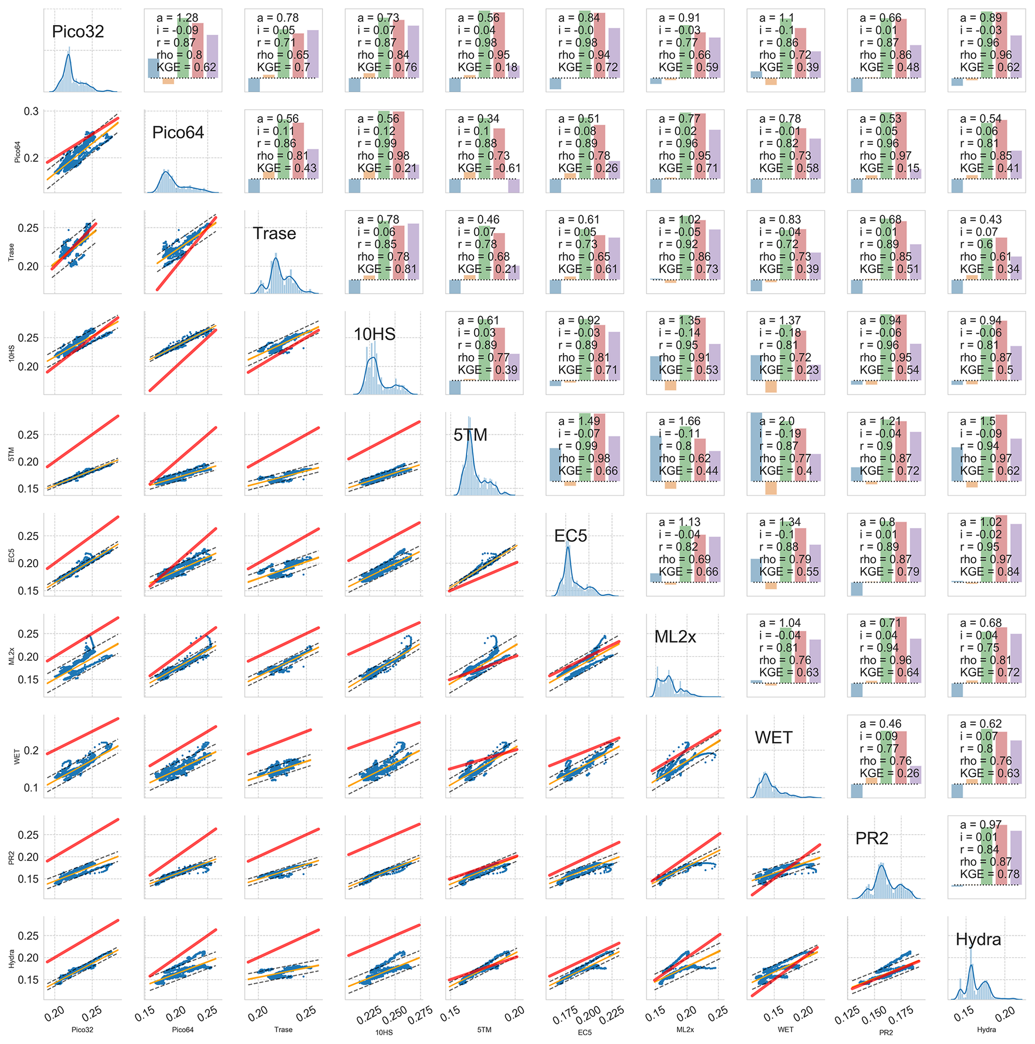
Figure 6Correlation matrix of all plausible sensor systems measuring soil moisture (given in m3 m−3). Diagonal panels give histogram and kernel density distribution of 0.5 h means of all sensors of one system. Lower half gives scatter plot (blue dots), linear regression (orange line), 0.95 predictive uncertainty bands (grey dashed lines) and the 1:1 line (red). The upper half reports the respective correlation measures, with a and i as scaling factor and intercept of the linear regression model, r as Pearson correlation coefficient, rho as Spearman rank correlation coefficient, and KGE as Kling–Gupta efficiency. These values are plotted as bars in the same order in the background, where a is plotted as deviation from unity.
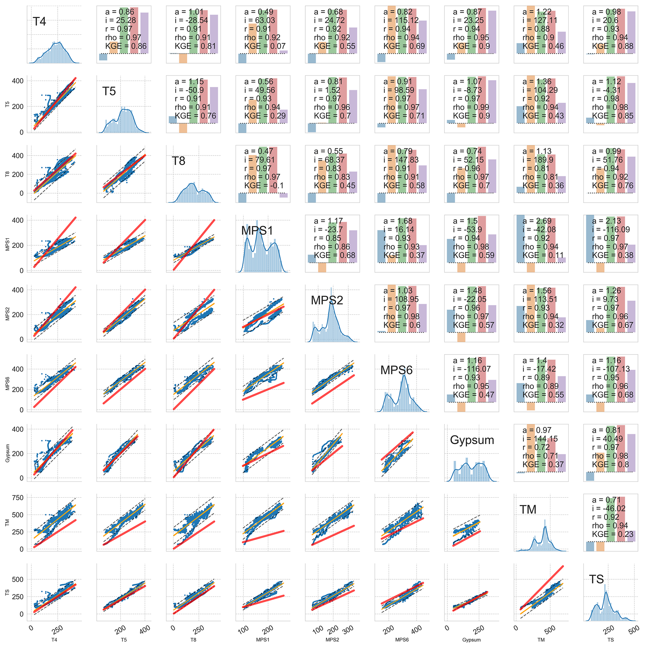
Figure 7Correlation matrix of all plausible sensor systems for matric potential (given in hPa). Diagonal panels give histogram and kernel density distribution of 0.5 h means of all sensors of one system. Lower half gives scatter plot (blue dots), linear regression (orange line), 0.95 predictive uncertainty bands (grey dashed lines) and the 1:1 line (red). The upper half reports the respective correlation measures, with a and i as scaling factor and intercept of the linear regression model, r as Pearson correlation coefficient, rho as Spearman rank correlation coefficient, and KGE as Kling–Gupta efficiency. These values are plotted as bars in the same order in the background, where a is plotted as deviation from unity and i is scaled with 0.01.
Figures 6 and 7 show the distribution plots of the means of each sensor system in the diagonal line. The lower panels show the scatter points (blue), the linear regression (orange line), the 0.95 predictive uncertainty bands (grey dashed lines) and the 1:1 line reference (red). In the upper panels the correlation measures are given as values and in a simple bar plot in the background. Here, a is plotted as the deviation from unity. High correlation is signalled when the first two bars are small and the last three bars are tall. The order of the reported systems is arbitrarily chosen without any implied ranking.
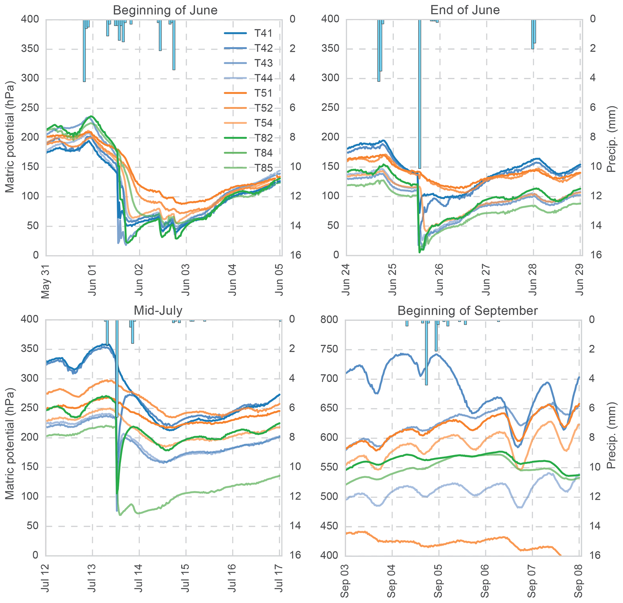
Figure 8Reactions of all tensiometers (T4, T5, T8) to four events. Emerging redistribution structures at the surface lead to growing deviation of the soil states across relatively short distances.
It should be noted that high or low correlation does not necessarily reflect the performance of a sensor system. Given the general assumption that TDR systems are superior, one might be interested in a comparison between the Pico and Trase systems. While the deviation from the 1:1 line is relatively small and moderate to high correlation exists, this is still far from being called a perfect match. The predictive uncertainty bands range around the often reported 3% vol accuracy. Other applications might use different sensors of the METER–Decagon family (10HS, 5TM, EC5), which are all based on the same impedance measurement principle but show substantial deviations in offset and scaling, too. Likewise, the high correlation but strong scaling of the TDR systems Pico32 and T3P (Fig. A1), which are based on the same technique, but with the former being a rod probe and the latter a tube probe, hints at a systematic issue (which led to a revision of the tube sensors already).
As seen in the time series plot (Fig. 4c), the tensiometers correlate very well. This is recovered in the correlation analysis (Fig. 7) with very high coefficients, although the offset might be an issue to look at. The indirect sensor systems using an equivalent porous medium present larger deviations but appear to be quite capable in general. Surprisingly, the developments in the MPS sensor family, which basically differ in the number of calibration points of the retention characteristics of the medium, do not show clear superiority to the latest MPS6. One should note the high offset for the MPS6 and TM compared to the tensiometers.
The sensing systems which did not deliver plausible data are shown in Appendix Figs. A1 and A2. It has to be highlighted that we cannot exclude issues with probe storage, installation failure or technical interferences leading to the registered performance. These systems can well be capable of outperforming other sensors when such issues are resolved. In addition, the systems which include a temperature sensor are reported in Appendix Fig. A3. There, high correlation of the records of most systems can be seen – except for systems which are not fully buried in the soil.
4.2 Evaluation of experimental hypotheses
We selected and prepared the site to be as homogenous as possible for an agricultural soil system. In order to evaluate the homogeneity assumption in our experiment, we focus on the reactions to some rain events over the monitoring period. We selected the tensiometers as the most direct measurement techniques as references for the soil water states. When comparing the individual sensor reaction to four rain events over 4 months, a strong deviation from the initially high congruency over time is apparent (Fig. 8). While the tensiometers recorded highly consistent values in the early phase of the experiment, the sensor readings divert irrespectively to their sensor system over the course of the experiment. Since we observed emerging redistribution structures at the surface, we attribute them to imprinting on the soil water states at 0.2 m depth. The effect of emerging structures on the overall system properties can also be seen in the in situ retention curves of some systems (which is left to further analyses).
Moreover, one has to be aware of the bare-soil field conditions, which resulted in relatively large diurnal temperature amplitudes in the soil, including related soil water processes and a potential exaggeration of local heterogeneity.
4.3 Data quality of soil water sensing
Overall, the data raise substantial questions about the data quality of state-of-the-art measurement systems of soil water content based on relative electrical permittivity of the bulk soil without specific, in situ calibration. Despite delivering plausible signals, neither the absolute values nor the relative reactions to events appear to be very accurate. Given the non-linear relation of gravimetric and TDR-sensed soil water content in the laboratory, and given the highly different monitoring records of the different TDR systems, the general belief of their superiority might deserve more detailed examination.
The a posteriori calibration approach did not succeed. To avoid disturbing the system, we did not take any soil samples at different states in the field, which could have been a better means for sensor calibration.
Although several studies evaluated soil moisture sensing systems (e.g. Walker et al., 2004; Mittelbach et al., 2011; Chow et al., 2009) and sensor calibration is known to be an issue (e.g. Rowlandson et al., 2013; Bogena et al., 2017; Rosenbaum et al., 2011), the scientific application still lacks a common procedure for evaluation and calibration of such data. When data from different sites and sensor systems are combined (e.g. Dorigo et al., 2011), our findings should raise awareness that deviations are not always a matter of soil heterogeneity.
Only few sensors allow for a recording of their raw signal. No sensor records the relative electrical permittivity of the bulk soil. However, the internal conversion functions and parameters are rarely accessible to the users. As the systems apply a higher-order polynomial function related to the Topp et al. (1980) equation, reverse calculation of the raw values or relative electrical permittivity is very difficult. For scientific application the sensor systems should provide such raw values as a prerequisite for a common calibration and evaluation procedure.
The data of the sensor comparison study are hosted in the PANGAEA repository (Jackisch et al., 2018, https://doi.org/10.1594/PANGAEA.892319). It is given under a Creative Commons License (CC BY-NC-SA 3.0) without any liability. The repository also holds a script (Sensor_Comparision_EEMD.ipynb) which provides direct access to general data visualisation and processing using Python given under a General Public License (GNU GPL 3).
The data reported in this study are intended to compare currently available systems for measurement of soil water content and matric potential under field conditions. While most systems did deliver plausible data, the records neither agree on a specific absolute value range nor are the relative values in accordance or rank-stable during events. Thus, mere plausibility checks of such data appear to be insufficient and cannot replace thorough calibration efforts and maintenance. Our findings point to substantial uncertainties for all types of sensing systems when the soil water sensors are applied without proper calibration. Unfortunately, the capability of laboratory reference measurements with exemplary sensors appears to be insufficient for a calibration. This issue becomes even more difficult to resolve given the observed reconfiguration of the system to a more heterogeneous state.
The following figures, Figs. A1, A2 and A3, are given to complement the general findings above.
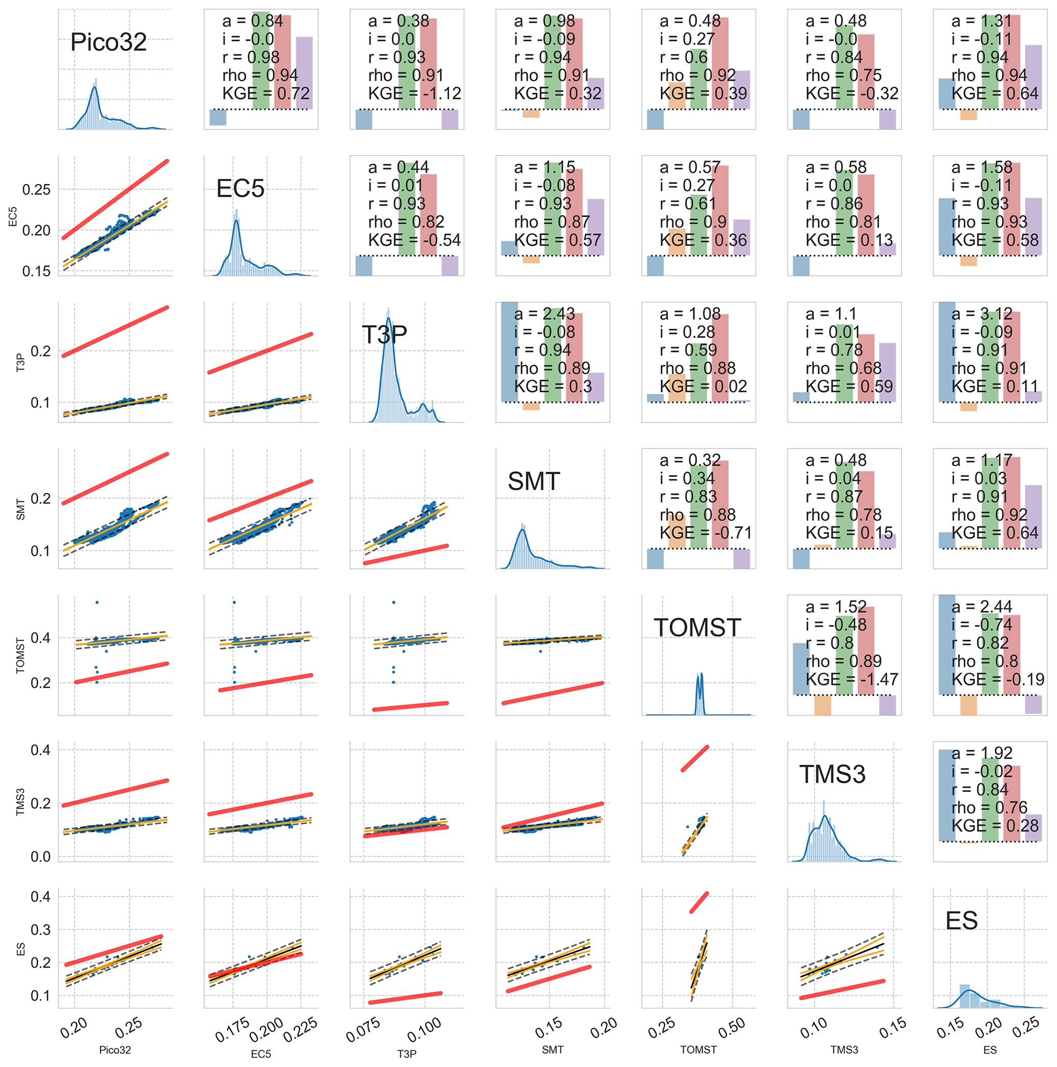
Figure A1Correlation matrix of two references and the less plausible soil moisture sensor systems (values given in m3 m−3). Diagonal panels give histogram and kernel density distribution of 0.5 h means of all sensors of one system. Lower half gives scatter plot (blue dots), linear regression (orange line), 0.95 predictive uncertainty bands (grey dashed lines) and the 1:1 line (red). The upper half reports the respective correlation measures, with a and i as scaling factor and intercept of the linear regression model, r as Pearson correlation coefficient, rho as Spearman rank correlation coefficient, and KGE as Kling–Gupta efficiency. These values are plotted as bars in the same order in the background, where a is plotted as deviation from unity. The ES system did not record data in the desired density (only 27 values compared, which is 0.5 % of the data series).
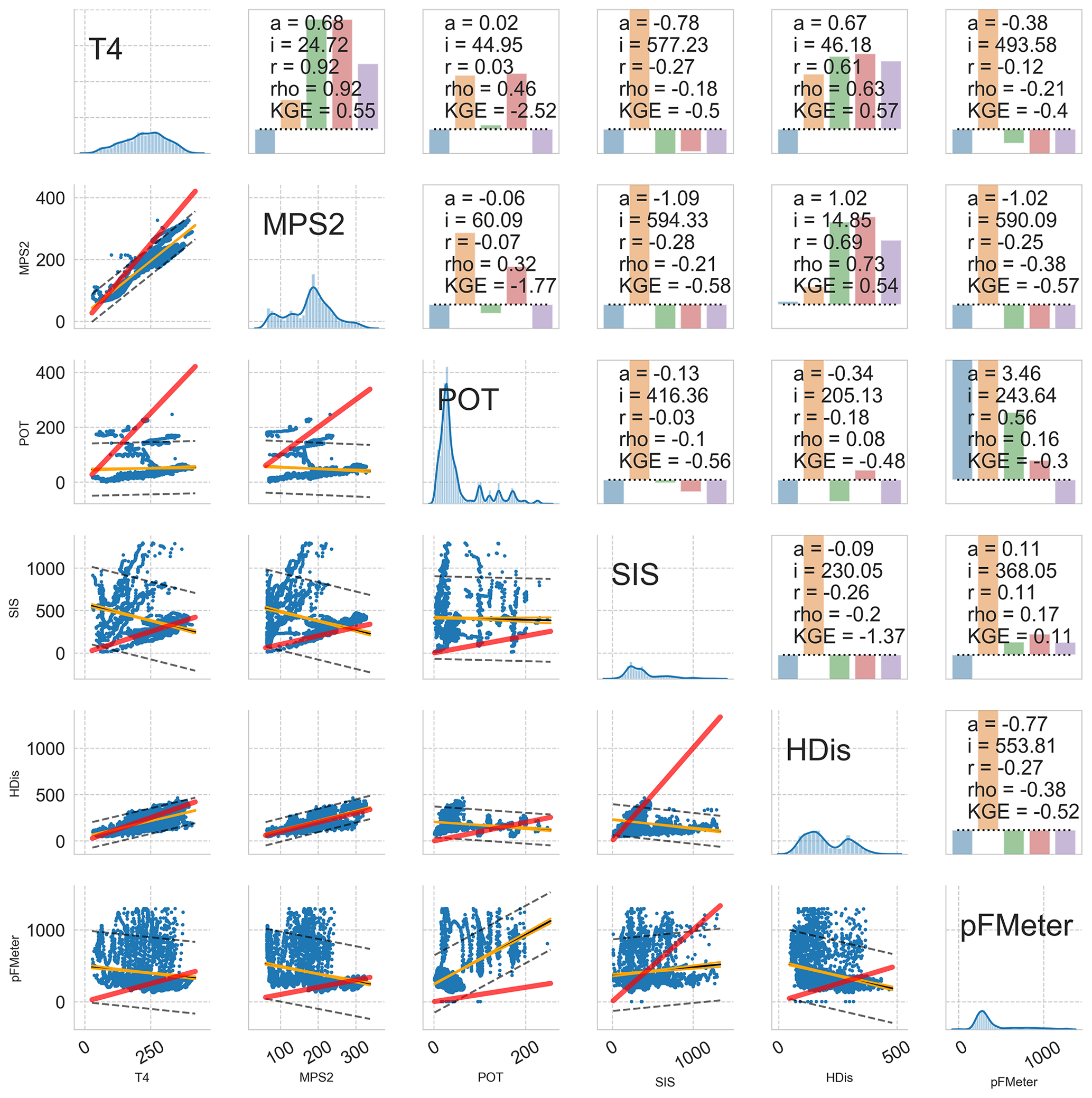
Figure A2Correlation matrix of two references and the less plausible sensor systems for matric potential (given in hPa). Diagonal panels give histogram and kernel density distribution of 0.5 h means of all sensors of one system. Lower half gives scatter plot (blue dots), linear regression (orange line), 0.95 predictive uncertainty bands (grey dashed lines) and the 1:1 line (red). The upper half reports the respective correlation measures, with a and i as scaling factor and intercept of the linear regression model, r as Pearson correlation coefficient, rho as Spearman rank correlation coefficient, and KGE as Kling–Gupta efficiency. These values are plotted as bars in the same order in the background, where a is plotted as deviation from unity and i is scaled with 0.01.
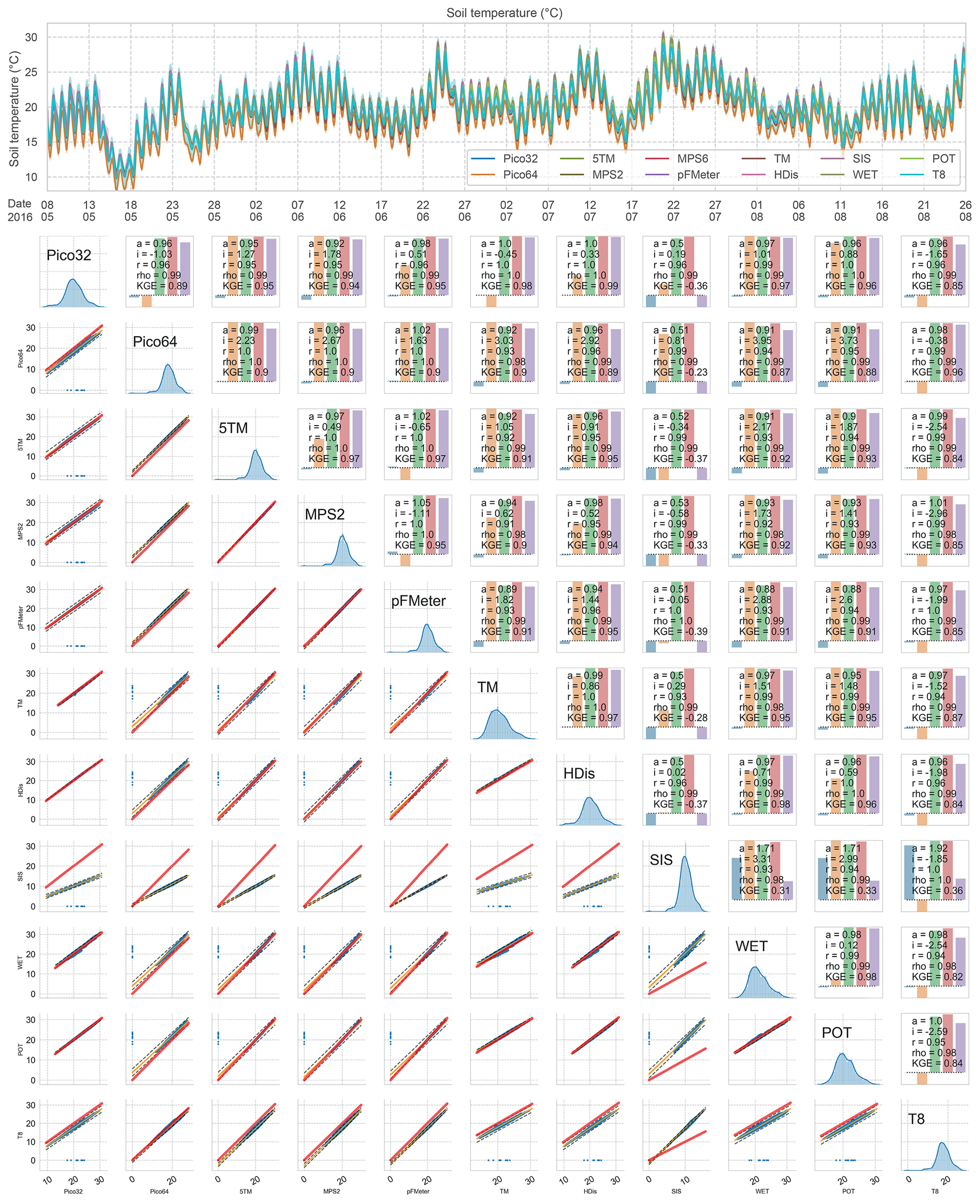
Figure A3Upper panel: time series of most recorded temperature values. Lower panels: correlation matrix of the sensor systems with temperature recording (given in ∘C). Diagonal panels give histogram and kernel density distribution of 0.5 h means of all sensors of one system. Lower half gives scatter plot (blue dots), linear regression (orange line), 0.95 predictive uncertainty bands (grey dashed lines) and the 1:1 line (red). The upper half reports the respective correlation measures, with a and i as scaling factor and intercept of the linear regression model, r as Pearson correlation coefficient, rho as Spearman rank correlation coefficient, and KGE as Kling–Gupta efficiency. These values are plotted as bars in the same order in the background, where a is plotted as deviation from unity.
All authors contributed to the fieldwork and data collection. WD, IA and KG designed the experimental set-up and primarily coordinated the field study. CJ and KG conducted the laboratory analyses. CJ compiled the data and performed the pre-analysis. CJ, KG, TG and WD wrote the paper. All authors contributed valuable feedback during this process.
The authors declare that they have no conflict of interest.
All data are reported as measured in the field and laboratory. We explicitly warn against using the data for nomination of any “best” system, as local heterogeneity, emerging surface structures, inappropriate storage of probes before installation, malfunction of single probes, and current revisions of hardware and software of the systems cannot be excluded. Some of the sensors have been upgraded by the manufacturers based on preliminary feedback from the comparison study already.
We gratefully acknowledge the cooperation in the sensor comparison study consortium. Especially the support of the Julius Kühn-Institut, Braunschweig, was indispensable to the study. We thank Heye Bogena and two anonymous referees for their constructive criticism on earlier versions of this paper and Giulio G. R. Iovine for steering the open review process.
This paper was edited by Giulio G. R. Iovine and reviewed by Heye Bogena and two anonymous referees.
Bakker, G., van der Ploeg, M. J., de Rooij, G. H., Hoogendam, C. W., Gooren, H. P. A., Huiskes, C., Koopal, L. K., and Kruidhof, H.: New Polymer Tensiometers: Measuring Matric Pressures Down to the Wilting Point, Vadose Zone J., 6, 196–202, https://doi.org/10.2136/vzj2006.0110, 2007. a
Bogena, H. R., Huisman, J. A., Schilling, B., Weuthen, A., and Vereecken, H.: Effective Calibration of Low-Cost Soil Water Content Sensors, Sensors, 17, 208, https://doi.org/10.3390/s17010208, 2017. a, b
Buckingham, E.: Studies on the movement of soil moisture, Bulletin (United States. Bureau of Soils) No. 38, Washington, availble at: http://www.worldcat.org/title/studies-on-the-movement-of-soil-moisture/oclc/29749917 (last access: 10 December 2019), 1907. a
Chow, L., Xing, Z., Rees, H. W., Meng, F., Monteith, J., and Lionel, S.: Field Performance of Nine Soil Water Content Sensors on a Sandy Loam Soil in New Brunswick, Maritime Region, Canada, Sensors, 9, 9398–9413, https://doi.org/10.3390/s91109398, 2009. a
Chudobiak, W. J., Syrett, B. A., and Hafez, H. M.: Recent Advances in Broad-Band VHF and UHF Transmission Line Methods for Moisture Content and Dielectric Constant Measurement, IEEE Trans. Instrum. Measure., 28, 284–289, https://doi.org/10.1109/TIM.1979.4314833, 1979. a
Davis, B. R., Lundien, J. R., and Williamson, A. N.: Feasibility study of the use of radar to detect surface and ground water, Tech. rep., US Army Engineer Waterways Experiment Station, Vicksburg, Mississippi, available at: http://cdm16021.contentdm.oclc.org/cdm/ref/collection/p266001coll1/id/2860 (last access: 10 December 2019), 1966. a
Dorigo, W. A., Wagner, W., Hohensinn, R., Hahn, S., Paulik, C., Xaver, A., Gruber, A., Drusch, M., Mecklenburg, S., van Oevelen, P., Robock, A., and Jackson, T.: The International Soil Moisture Network: a data hosting facility for global in situ soil moisture measurements, Hydrol. Earth Syst. Sci., 15, 1675–1698, https://doi.org/10.5194/hess-15-1675-2011, 2011. a
Gardner, W. and Widtsoe, J. A.: The Movement of Soil Moisture, Soil Sci., 11, 215–232, available at: https://journals.lww.com/soilsci/Fulltext/1921/03000/THE_MOVEMENT_OF_SOIL_MOISTURE.3.aspx (last access: 10 December 2019), 1921. a
Geiger, F. E. and Williams, D.: Dielectric constants of soils at microwave frequencies, available at: http://ntrs.nasa.gov/search.jsp?R=19720021782 (last access: 10 December 2019), 1972. a
Jackisch, C., Andrä, I., Germer, K., Schulz, K., Schiedung, M., Haller-Jans, J., Schneider, J., Jaquemotte, J., Helmer, P., Lotz, L., Graeff, T., Bauer, A., Hahn, I., Sanda, M., Kumpan, M., Dorner, J., de Rooij, G., Wessel-Bothe, S., Kottmann, L., Schittenhelm, S., and Durner, W.: Soil moisture and matric potential – An open field comparison of sensor systems, PANGAEA, https://doi.org/10.1594/PANGAEA.892319, 2018. a, b, c
Loewer, M., Günther, T., Igel, J., Kruschwitz, S., Martin, T., and Wagner, N.: Ultra-broad-band electrical spectroscopy of soils and sediments – a combined permittivity and conductivity model, Geophys. J. Int., 210, 1360–1373, https://doi.org/10.1093/gji/ggx242, 2017. a
Mittelbach, H., Casini, F., Lehner, I., Teuling, A. J., and Seneviratne, S. I.: Soil moisture monitoring for climate research: Evaluation of a low-cost sensor in the framework of the Swiss Soil Moisture Experiment (SwissSMEX) campaign, J. Geophys. Res.-Solid Earth, 116, L18405, https://doi.org/10.1029/2010JD014907, 2011. a
Or, D.: Who Invented the Tensiometer?, Soil Sci. Soc. Am. J., 65, 1, https://doi.org/10.2136/sssaj2001.6511, 2001. a
Owen, B. B., Miller, R. C., Milner, C. E., and Cogan, H. L.: The Dielectric Constant of Water as a Function of Temperature and Pressure, The J. Phys. Chem., 65, 2065–2070, https://doi.org/10.1021/j100828a035, 2002. a
Ponizovsky, A. A., Chudinova, S. M., and Pachepsky, Y. A.: Performance of TDR calibration models as affected by soil texture, J. Hydrol., 218, 35–43, https://doi.org/10.1016/S0022-1694(99)00017-7, 1999. a
Rosenbaum, U., Huisman, J. A., Vrba, J., Vereecken, H., and Bogena, H. R.: Correction of Temperature and Electrical Conductivity Effects on Dielectric Permittivity Measurements with ECH2O Sensors, Vadose Zone J., 10, 582–593, https://doi.org/10.2136/vzj2010.0083, 2011. a, b
Roth, K., Schulin, R., Flühler, H., and Attinger, W.: Calibration of time domain reflectometry for water content measurement using a composite dielectric approach, Water Resour. Res., 26, 2267–2273, https://doi.org/10.1029/WR026i010p02267, 1990. a
Rowlandson, T. L., Berg, A. A., Bullock, P. R., Ojo, E. R., McNairn, H., Wiseman, G., and Cosh, M. H.: Evaluation of several calibration procedures for a portable soil moisture sensor, J. Hydrol., 498, 335–344, https://doi.org/10.1016/j.jhydrol.2013.05.021, 2013. a
Schwartz, R. C., Casanova, J. J., Pelletier, M. G., Evett, S. R., and Baumhardt, R. L.: Soil Permittivity Response to Bulk Electrical Conductivity for Selected Soil Water Sensors, Vadose Zone J., 12, 1–13, https://doi.org/10.2136/vzj2012.0133, 2013. a
Soilmoisture Equipment inc.: Trase Operating Instructions, available at: https://www.soilmoisture.com/pdfs/Resource_Instructions_0898-6050_6050 X1 Trase Full Ops. Manual 2000.pdf (last access: 10 December 2019), 1996. a
Stacheder, M., Fundinger, R., and Koehler, K.: On-Site Measurement of Soil Water Content by a New Time Domain Reflectometry (TDR) Technique, in: Field Screening Europe, 161–164, Springer, Dordrecht, Dordrecht, https://doi.org/10.1007/978-94-009-1473-5_37, 1997. a
Topp, G., Davis, J., and Annan, A.: Electromagnetic determination of soil water content: Measurements in coaxial transmission lines, Water Resour. Res., 16, 574–582, https://doi.org/10.1029/WR016i003p00574, 1980. a
van der Ploeg, M. J., Gooren, H. P. A., Bakker, G., Hoogendam, C. W., Huiskes, C., Koopal, L. K., Kruidhof, H., and de Rooij, G. H.: Polymer tensiometers with ceramic cones: direct observations of matric pressures in drying soils, Hydrol. Earth Syst. Sci., 14, 1787–1799, https://doi.org/10.5194/hess-14-1787-2010, 2010. a
Van Genuchten, M. T.: Closed-Form Equation for Predicting the Hydraulic Conductivity of Unsaturated Soils, Soil Sci. Soc. Am. J., 44, 892–898, 1980. a
Walker, J. P., Willgoose, G. R., and Kalma, J. D.: In situ measurement of soil moisture: a comparison of techniques, J. Hydrol., 293, 85–99, https://doi.org/10.1016/j.jhydrol.2004.01.008, 2004. a
Wang, J. R. and Schmugge, T. J.: An Empirical Model for the Complex Dielectric Permittivity of Soils as a Function of Water Content, Geoscience and Remote Sensing, IEEE Trans., GE-18, 288–295, https://doi.org/10.1109/TGRS.1980.350304, 1980. a
Wild, J., Kopecký, M., Macek, M., Sanda, M., Jankovec, J., and Haase, T.: Climate at ecologically relevant scales: A new temperature and soil moisture logger for long-term microclimate measurement, Agr. Forest Meteorol., 268, 40–47, https://doi.org/10.1016/j.agrformet.2018.12.018, 2019. a
Wraith, J. M. and Or, D.: Temperature effects on soil bulk dielectric permittivity measured by time domain reflectometry: Experimental evidence and hypothesis development, Water Resour. Res., 35, 361–369, https://doi.org/10.1029/1998WR900006, 1999. a