the Creative Commons Attribution 4.0 License.
the Creative Commons Attribution 4.0 License.
 | 20 Apr 2020
Sval_Imp: a gridded forcing dataset for climate change impact research on Svalbard
Thomas Vikhamar Schuler
Torbjørn Ims Østby
We present Sval_Imp, a high-resolution gridded dataset designed for forcing models of terrestrial surface processes on Svalbard. The dataset is defined on a 1 km grid covering the archipelago of Svalbard, located in the Norwegian Arctic (74–82∘ N). Using a hybrid methodology, combining multidimensional interpolation with simple dynamical modeling, the atmospheric reanalyses ERA-40 and ERA-Interim by the European Centre for Medium-Range Weather Forecasting have been downscaled to cover the period 1957–2017 at steps of 6 h. The dataset is publicly available from a data repository. In this paper, we describe the methodology used to construct the dataset, present the organization of the data in the repository and discuss the performance of the downscaling procedure. In doing so, the dataset is compared to a wealth of data available from operational and project-based measurements. The quality of the downscaled dataset is found to vary in space and time, but it generally represents an improvement compared to unscaled values, especially for precipitation. Whereas operational records are biased to low elevations around the fringes, we stress the hitherto underused potential of project-based measurements at higher elevation and in the interior of the archipelago for evaluating atmospheric models. For instance, records of snow accumulation on large ice masses may represent measures of seasonally integrated precipitation in regions sensitive to the downscaling procedure and thus providing added value.
Sval_Imp (Schuler, 2018) is publicly available from the Norwegian Research Data Archive NIRD, a data repository (https://doi.org/10.11582/2018.00006).


The nonlinearity of many surface processes poses challenges in terms of the appropriateness of atmospheric forcing for impact studies in terms of accuracy and precision (e.g., Liston and Elder, 2006). Especially in mountainous areas, the variability of surface systems is typically governed by spatial scales not resolved in regional climate models, and adjustments have to be made to overcome this (e.g., Fiddes and Gruber, 2014). A variety of methods have been developed for this purpose, differing in terms of data requirements and computational cost. While empirical–statistical scaling requires reference data for training and assumes a temporal robustness of the employed statistical relations (e.g., Ehret et al., 2012; Maraun, 2013), dynamic downscaling by means of high-resolution atmospheric modeling has high computational costs (e.g., Gutmann et al., 2016).
In this paper, we present Sval_Imp (Schuler, 2018), a high-resolution gridded dataset obtained using a hybrid methodology combining multidimensional interpolation with simple dynamical modeling. The dataset is defined on a 1 km grid covering the archipelago of Svalbard, located in the Norwegian Arctic (74–82∘ N, 10–35∘ E). The atmospheric reanalyses ERA-40 and ERA-Interim by the European Centre for Medium-Range Weather Forecasting have been downscaled to cover the period 1957–2017 at 6 h temporal resolution. The dataset comprises the near-surface variables required to compute the surface energy balance, namely air temperature, precipitation, relative humidity, wind speed, and downwelling components of shortwave (solar) and longwave (thermal) radiation. Sval_Imp is publicly available from the Norwegian Research Data Archive NIRD, a data repository (https://doi.org/10.11582/2018.00006, Schuler, 2018). In the following, we describe the methodology used to derive the dataset, present the organization of the data in the repository and discuss the performance of the downscaling procedure. For the latter, the dataset is compared to a wealth of data available from long-term operational and short-term scientific records of meteorological and glaciological measurements. Operational records are biased to low elevations around the fringes of the archipelago. Therefore, we stress the hitherto underused potential of project-based measurements in the interior, high-elevation regions for evaluating atmospheric models. For instance, records of snow accumulation on large ice masses may represent measures of seasonally integrated precipitation in regions sensitive to the downscaling procedure, thus providing added value. Sval_Imp has been employed entirely or in part by a range of projects for forcing process models of the surface energy and mass balances of glaciers (Østby et al., 2017) and precipitation patterns and meltwater production in the Kongsfjord area (Pramanik et al., 2018), for assimilation of remotely sensed snow cover using a snow distribution model (Aalstad et al., 2018), and assessing growing conditions for fungi (Botnen, 2020). Further, the dataset has been used to assess changes and trends in climate conditions of Svalbard (Hanssen-Bauer et al., 2019).
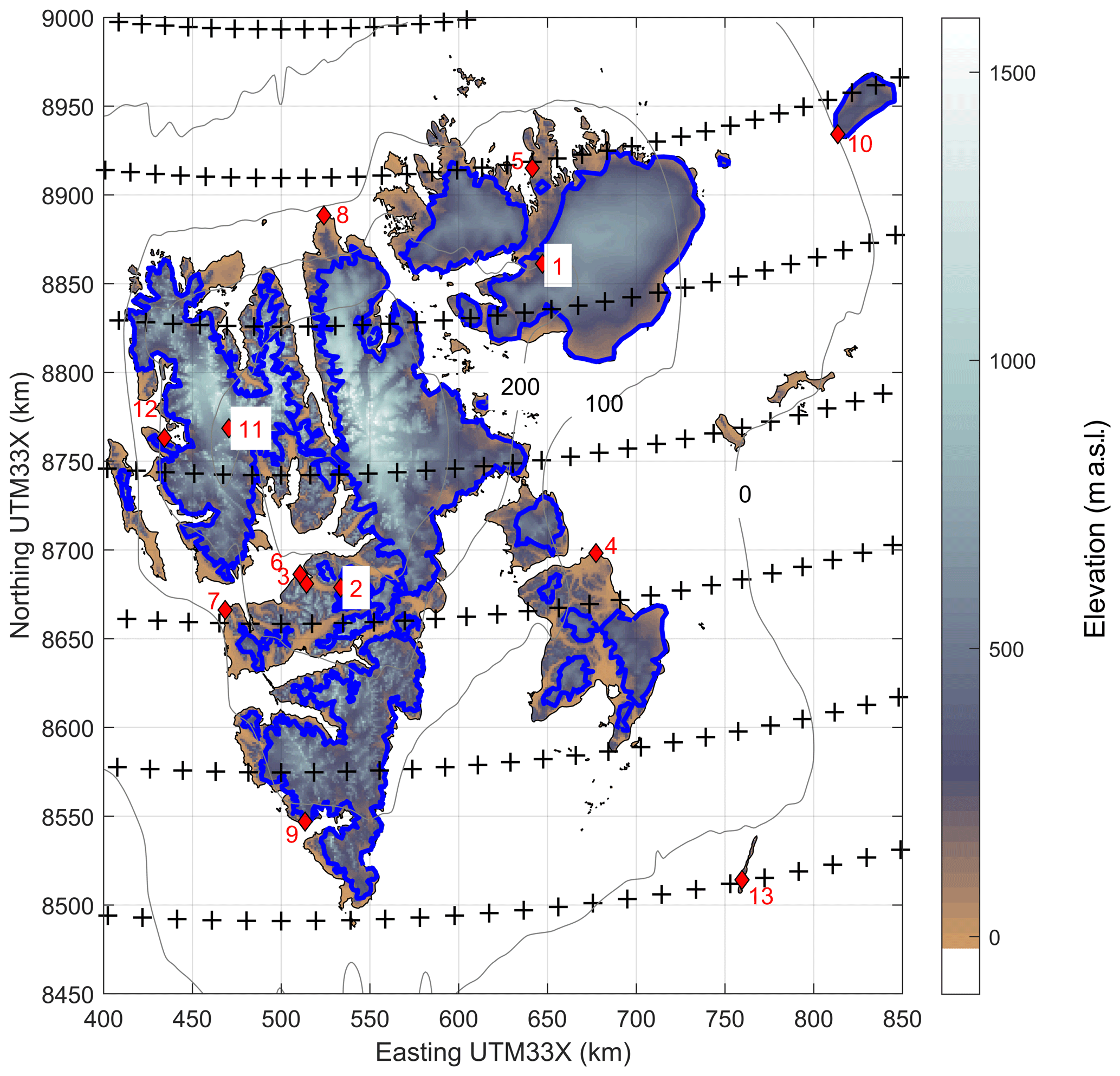
Figure 1The map shows the Svalbard archipelago, shading indicates surface elevation, and glacierized areas are outlined in blue. The locations of meteorological stations are represented by red diamonds, and the numbers refer to the station names: 1 – Etonbreen; 2 – Janssonhaugen; 3 – Gruvefjellet; 4 – Kapp Heuglin; 5 – Rijpfjorden; 6 – Svalbard Airport; 7 – Isfjord Radio; 8 – Verlegenhuken; 9 – Hornsund; 10 – Kvitøya; 11 – Holtedahlfonna; 12 – Ny-Ålesund; 13 – Hopen. The black crosses indicate the grid points of the ERA reanalyses, and the grey contour lines indicate the topography of Svalbard in the ERA reanalyses at 0, 100, 200 and 300 m a.s.l.
To generate fields of near-surface air temperature, precipitation, relative humidity, wind, and downwelling shortwave and longwave radiation, we have downscaled the ERA-40 and ERA-Interim reanalyses of the European Centre for Medium-Range Weather Forecasts (Uppala et al., 2005; Dee et al., 2011). The reanalysis data are provided at 6 h intervals and have been retrieved on a spatial grid covering the periods 1957–2002 (ERA-40) and 1979–2017 (ERA-Interim). These data have been downscaled to a 1 km grid covering the region of interest (Fig. 1) using the scheme described in the following to produce Sval_Imp, a high-resolution, 6 h dataset of precipitation, temperature, relative humidity, wind speed, and downwelling shortwave and longwave radiation fluxes.
2.1 Downscaling
Precipitation is often heavily biased in coarsely resolved reanalyses, especially in environments with pronounced topography, where it typically is too low and lacks spatial detail (Schuler et al., 2008). This is associated with the smoothed representation of the actual topography in the large-scale model used for the reanalysis (Fig. 1), leading to an underestimation of orographic precipitation. Figure 1 shows that ERA greatly generalizes the high-resolution topography, representing Svalbard as a wide and flat bump that exceeds sea-level far off the actual coastlines, while surface elevation in the interior does not exceed 400 m a.s.l. In contrast, the highest elevation in our gridded topography map is 1600 m a.s.l. The roughness of the actual topography that gave rise to the name of the main island “Spitsbergen” (pointed mountains) is not represented by the smoothed topography used for the ERA reanalyses. We assume that this is the main reason for the poor performance of reanalyzed precipitation. To account for orographic enhancement, we use a linear theory (LT) of orographic precipitation (Smith and Barstad, 2004).
The other required climate variables are downscaled to the 1 km grid largely following the TopoSCALE methodology (Fiddes and Gruber, 2014), which also builds on the assumption that weaknesses in the representation of topography at the coarse scale are mainly responsible for the misfit between coarse-scale and point observations. TopoSCALE exploits the relatively high vertical resolution of the reanalysis data to downscale variables to the elevation of the actual topography, based on the properties of the vertical structure in the reanalysis. The downscaled fields preserve the horizontal gradients present in ERA but include additional features caused by the real topography that were not present in the ERA products. In doing so, we add spatial detail to the reanalysis fields that is consistent with the temporal evolution of atmospheric conditions of the reanalysis. This approach is assumed to outperform simpler bias corrections, since transient properties of the atmosphere are accounted for. For example, transient lapse rates including inversions in the reanalysis data will be preserved in the downscaled product.
In our application, we modified the TopoSCALE methodology regarding downscaling of direct shortwave radiation and air temperature, as described in Sect. 2.3 and 2.4.
2.2 Precipitation
The LT model describes an air parcel as it moves across a prescribed surface topography. The air parcel is characterized by its temperature, stability, wind direction and speed. Terrain-induced uplift of the air parcel results in condensation and eventually precipitation of moisture downstream of the uplift. This model has been successfully evaluated using precipitation gauges (Barstad and Smith, 2005) and snow measurements (Schuler et al., 2008; Østby et al., 2017) and applied for downscaling precipitation (e.g., Crochet et al., 2007; Jarosch et al., 2012; Roth et al., 2018). The linear theory utilizes a Boussinesq description of mountain wave to derive a transfer function that, for given wind conditions, relates the orographically enhanced precipitation to terrain topography.
By using spectral decomposition and algebraic manipulation, Smith and Barstad (2004) derived the following transfer function:
relating , the Fourier transform of the precipitation enhancement, to the Fourier transform of terrain elevation , with k and l being the horizontal wave numbers. This relation depends on the uplift sensitivity factor Cw, thickness of the moist layer Hw, the intrinsic frequency (U and V being the east and north components of the wind vector), and the conversion and fallout timescales τc and τf, respectively. In Eq. (1), the vertical wave number m controls the depth and tilt of the forced air uplift and is a function of the moist Brunt–Väisälä frequency, Nm, a quantity describing atmospheric stability.
Precipitation rates are obtained by retransforming and adding it to the background precipitation P∞, which accounts for large-scale frontal and convective precipitation separate from orographic precipitation Poro. P∞ has been corrected for the orographic effect already present in the ERA reanalyses Poro(hERA) by estimating this effect applying Eq. (1) to the large-scale topography hERA and removing the result from the ERA precipitation (Schuler et al., 2008). Total precipitation, Ptotal, is then
Since the theory assumes saturated conditions, we account for reduced orographic enhancement at lower humidity by adopting a correction factor f proposed by Sinclair (1994):
which suppresses orographic enhancement when RH <0.8.
Instead of treating Nm, τf and τc as adjustable, constant parameters, we exploit the evolution of the moisture-bearing layer of the atmosphere described in the reanalyses to derive transient values. In doing so, we remove calibration parameters from our method and enable weather-dependent variation in Nm, τf and τc. Values of Nm are calculated as follows:
where g is gravitational acceleration and is vertically averaged air temperature weighted by the moisture content at several pressure levels (Jarosch et al., 2012). Environmental lapse rates Γe are derived from air temperature at 700 and 850 hPa and corresponding geopotential heights. Γm is the moist adiabatic lapse rate, calculated according to Stone and Carlson (1979) using vertically averaged values of atmospheric properties from the reanalyses weighted by moisture content. This follows the convention that a positive lapse rate represents cooling with increasing elevation. Barstad and Smith (2005) report that typical values of Nm range between 0 s−1, representing an atmosphere with no stratification, and 0.01 s−1, representing a stably stratified atmosphere. To avoid conditions inconsistent with the assumptions of the theory, we limit Nm to this range. The quantities Hw, Cw and m are derived from Nm (Smith and Barstad, 2004).
Advection timescales τc and τf are assumed equal, and is derived from the thickness of the moist layer Hw and accounting for a typical hydrometeor fall speed v, which is taken as constant but allowed to take different values for solid and liquid hydrometeors. This phase transition is determined by a threshold temperature of 273 K, hence v(T≤273 K) =1 m s−1 for solid and v(T>=273 K) =2 m s−1 for liquid precipitation. In Eq. (1), terrain elevation h is the only gridded variable, the other variables represent averages over the volume of the described air parcel. To characterize this air parcel, we first vertically average the values defined at the nodes of the horizontal domain over the 700 and 850 hPa pressure levels weighted by the moisture content of the individual layers. These vertically averaged values are then horizontally averaged over an area defined by a 200 km buffer around the 200 m contour of the reanalysis topography, the latter roughly outlining the extent of the archipelago (Fig. 1).
This setup is then applied to each 6 h time step, and the resulting time slices are progressively added to the record.
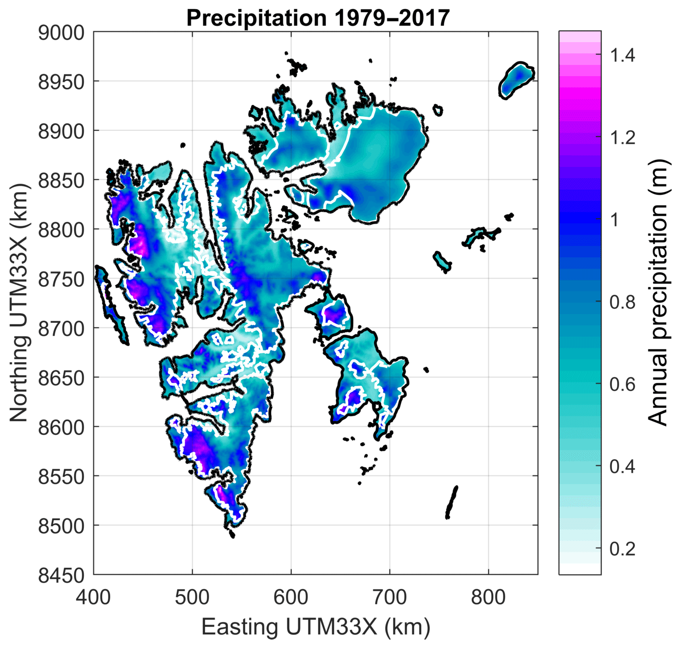
Figure 2Example plot of long-term mean annual precipitation (m) over 1979–2017, downscaled from ERA-Interim.
2.3 Air temperature
The downscaling for near-surface air temperature at the 2 m level (T2 m) closely follows the TopoSCALE procedure of Fiddes and Gruber (2014), thereby we assume that the vertical structure of the free atmosphere determines the distribution of T2 m with terrain elevation. For each 6 h time step, T2 m is derived from a three-dimensional interpolation of the vertical air temperature structure of the large-scale reanalysis to the location of the grid nodes representing the high-resolution terrain elevation. We notice that for a melting snow or ice surface, skin temperature is bounded to 273 K, influencing the near surface air temperature and resulting in reduced along-surface air temperature lapse rates (e.g., Marshall et al., 2007). To account for this effect, we apply a simple horizontal interpolation of the two-dimensional T2 m from the ERA reanalysis field, where T2 m>273 K, instead of interpolating a three-dimensional data volume to the surface elevation of the high-resolution topography. This strategy is motivated by the discovery of unrealistic warm air temperatures at higher elevations in a test application. The occurrence of this unphysical temperature inversion was restricted to the melting period, caused by extrapolation of surface inversions close to a snow and/or ice surface, the temperature of which is capped at 273 K. To avoid this effect, we assume that where T2 m>273 K, the T2 m of the reanalysis is consistent with a melting surface and hence more realistic than a free-atmosphere interpolation.
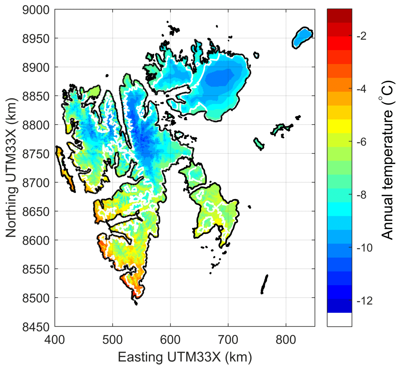
Figure 3Example plot of mean air temperature (2 m) in ∘C, over the period 1979–2017, downscaled from ERA-Interim.
2.4 Radiation
Downscaling of shortwave and longwave downwelling radiative fluxes (SW and LW, respectively) was conducted by adopting the TopoSCALE methodology (Fiddes and Gruber, 2014) with a few adjustments. The shortwave radiation at the surface level of the reanalysis is projected to the high-resolution topography in a three-step procedure: first the surface SW flux is separated into direct and diffuse components; second, the direct component is corrected for the elevation difference between the reanalysis surface and the high-resolution topography, considering an effective atmospheric transmissivity that is derived from top-of-atmosphere and surface fluxes; third, a topographic correction is applied to account for effects of slope and aspect of the high-resolution topography, as well as shading by surrounding topography. To compute direct solar radiation we apply the relationship of Kumar et al. (1997) for atmospheric attenuation rather than the one given by Fiddes and Gruber (2014). Solar geometry variables such as solar zenith and azimuth and topographic shading due to local slope and aspect are calculated following Reda and Andreas (2004). Cast shadow and hemispherical obstructions caused by surrounding topography are calculated following Ratti (2001). The longwave surface flux is downscaled by correcting for the elevation difference between reanalysis and high-resolution grids using an atmospheric emissivity. This emissivity is estimated by accounting for a clear-sky component that depends on humidity and air temperature and a cloud component that is estimated from the difference between the clear-sky component and the reanalysis longwave flux. Further terrain effects are incorporated through multiplication with the sky-view factor.
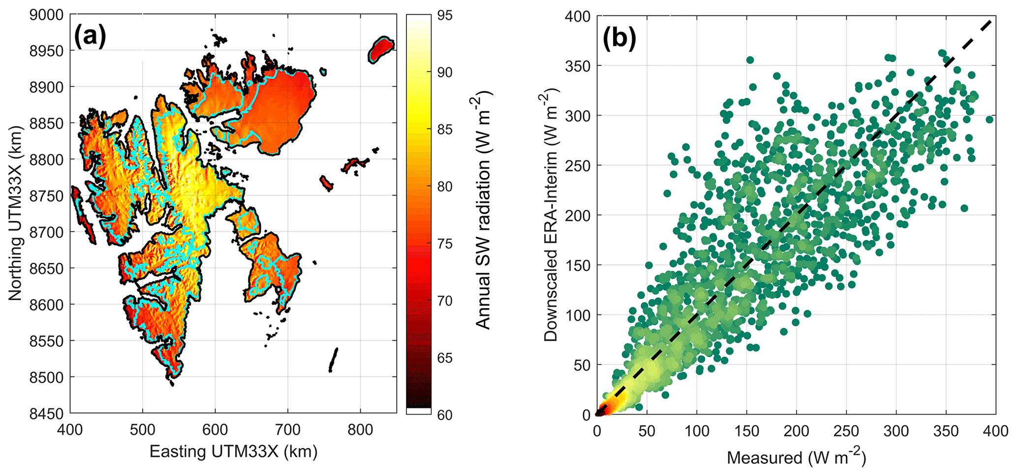
Figure 4(a) Example plot of 1979–2017 incident shortwave radiation (W m−2), downscaled from ERA-Interim. (b) Comparison between measured (Maturilli et al., 2015) and downscaled daily values of SW at Ny-Ålesund. The color indicates the density of points from red (high) to green (low).
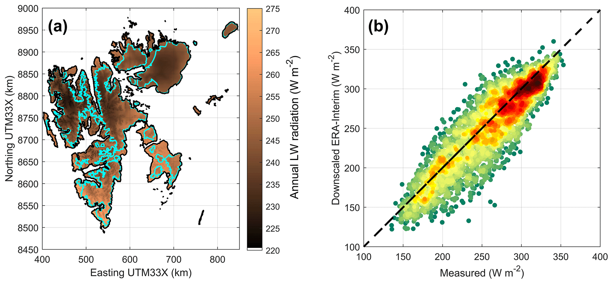
Figure 5(a) Example plot of 1979–2017 downwelling longwave radiation (W m−2), downscaled from ERA-Interim. (b) Comparison between measured (Maturilli et al., 2015) and downscaled daily values of LW at Ny-Ålesund. The color indicates the density of points from red (high) to green (low).
2.5 Relative humidity and wind speed
Similar to our assumption about T2 m over a melting surface, we suggest that wind speed and RH in the boundary layer are more affected by surface rather than by free-atmosphere conditions, and we hence apply a simple two-dimensional interpolation of the near-surface values of the reanalysis, instead of interpolating a three-dimensional data volume to the surface elevation of the high-resolution topography.
Østby et al. (2017) and Vikhamar-Schuler et al. (2019) have conducted thorough evaluations of the Sval_Imp dataset using data from meteorological stations. Here, we summarize their main results in the subsequent subsections and refer to Østby et al. (2017) for details. Furthermore, we present additional evaluation of the precipitation using snow measurements. Typically, meteorological records are available as daily mean values, and 6-hourly, downscaled variables have been temporally aggregated to match the time step of measurements. Precipitation in reanalysis is not constrained by data assimilation, giving rise to uncertainty in timing and amount. Our downscaling aims to reduce the bias in precipitation amount but does not treat the timing. For a performance evaluation, we therefore use monthly precipitation sums, which are regarded as robust against timing mismatches, whereas a higher temporal resolution could penalize a method that otherwise is successful in reducing the underestimation of the reanalysis.
3.1 Precipitation
At the operational weather stations (Fig. 1), downscaled precipitation (Fig. 2) is overestimated by 5 to 25 mm per month at the weather stations, with a slightly higher bias during winter (Table 1). This is also consistent with the findings of Vikhamar-Schuler et al. (2019), who evaluated the performance at six weather stations for several 30-year reference periods (1961–1990, 1971–2000 and 1988–2017). These biases are partly caused by precipitation measurements that are too low, the values of which are heavily affected by wind-induced undercatch, especially for solid precipitation. Førland and Hanssen-Bauer (2000) suggest that for solid precipitation, the actual precipitation at wind-exposed sites may be up to 80 % higher than the gauge record. A newly developed correction scheme for Norwegian mountain environments (Wolff et al., 2015) supports the finding of a large undercatch for solid precipitation; however, this correction has not yet been applied for Arctic conditions in Svalbard.
In addition to gauge measurements from low-elevation stations along the coast, we also used snow survey transects across Austfonna, a large ice cap in northeastern Svalbard (Fig. 1), to evaluate the Sval_Imp precipitation. We suggest that snow deposition on large glacier areas, measured at the end of the winter, represents seasonally integrated precipitation. While these measurements do not allow temporal resolution below one snow season (typically October–May), they provide useful information about spatial precipitation patterns in areas and elevations not covered by the operational meteorological stations. This approach builds on the implicit assumption of negligible sublimation, such that accumulated snow water equivalent represents the sum of precipitation over the winter season. Svalbard has high air humidity throughout the year, limiting the potential for sublimation. In an energy-balance study, Østby et al. (2017) estimated sublimation to about 0.016 , which is 1–2 orders of magnitude smaller than typical annual precipitation sums. There is generally good agreement concerning the spatial pattern across the Austfonna ice cap (Fig. 6), where snow accumulation reveals a distinctive southeast–northwest asymmetry (Taurisano et al., 2007; Schuler et al., 2007; Dunse et al., 2009) caused by orographic enhancement of precipitation coming from the southeast sector (i.e., the Barents Sea), although in individual years the downscaled values underestimate the measured accumulation, especially in 2007 (Fig. 6). Even though there is considerable scatter between observed and downscaled winter precipitation, there is positive correlation, indicating that the spatial pattern is matched and in most years there is no systematic bias, showing that the overall precipitation amount is adequately represented. On the other hand, the unscaled ERA-Interim winter precipitation shows almost no spatial variation and considerably underestimates observed values (Fig. 2).
Østby et al. (2017) found that the winter mass balance of Hansbreen, a glacier close to Hornsund, was not well reproduced, both in terms of spatial pattern and accumulation amount. Aas et al. (2016) similarly reported the lowest performance for Hansbreen, although they used a much more complex precipitation scheme than the one presented here. The generally low performance of several precipitation distribution schemes compared to the Hansbreen record has been interpreted to result from local conditions at Hansbreen, where the spatial distribution of snow is caused by wind redistribution rather than by the spatial precipitation pattern (Grabiec et al., 2006).
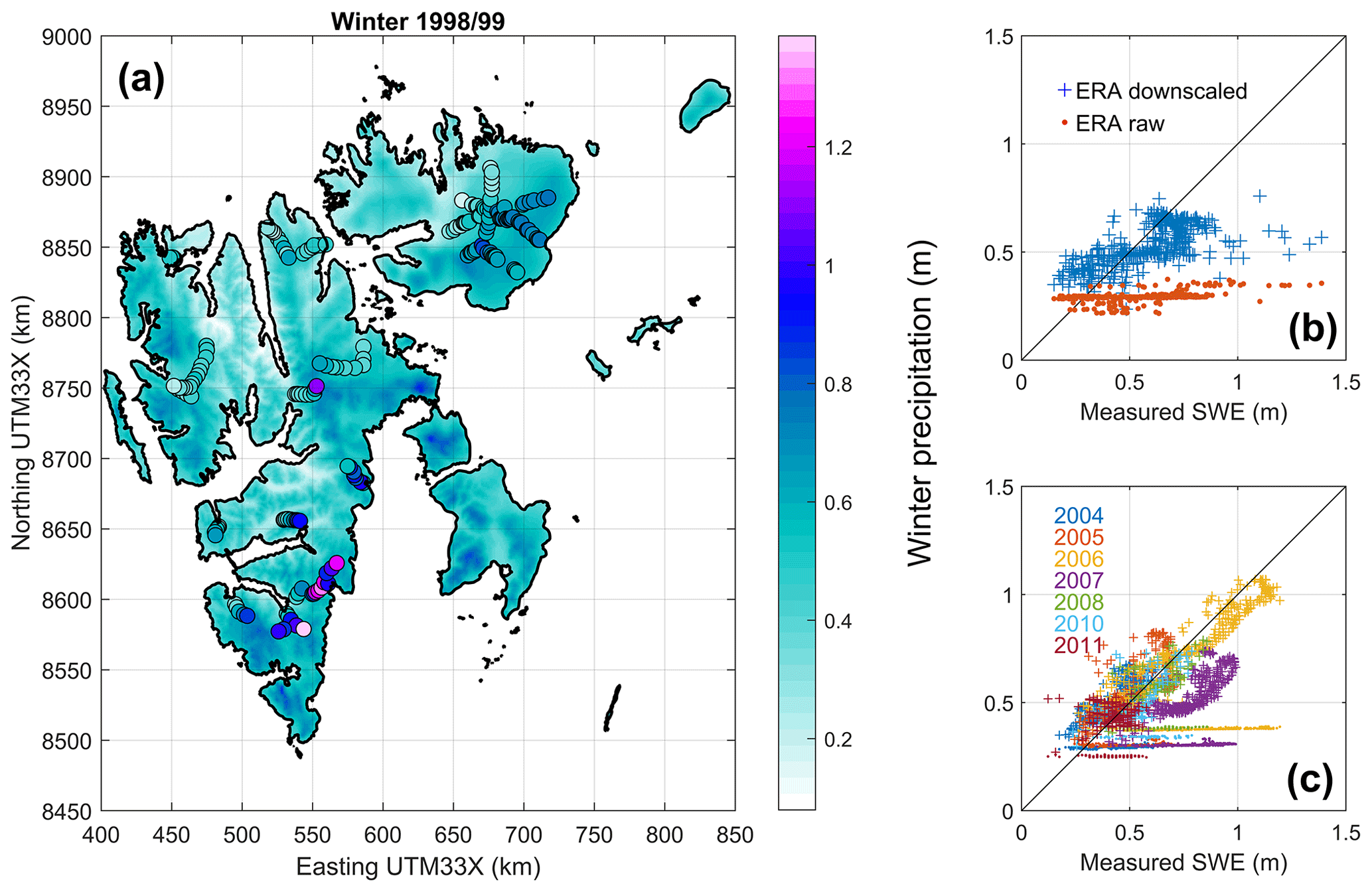
Figure 6(a) Map view of Sval_Imp precipitation accumulated over October 1998 to March 1999, overlaid with colored circles that indicate the measured snow water equivalent (SWE) by Sand et al. (2003). (b) Scatterplot comparing the 1999 measurements to winter precipitation according to Sval_Imp (crosses) and ERA-Interim (dots). (c) A similar scatterplot to (b) but only for the Austfonna dataset, which provides multi-temporal coverage (Taurisano et al., 2007; Dunse et al., 2009).
3.2 Air temperature
Downscaled air temperatures (Fig. 3) are compared to observations at the meteorological stations listed in Table 1 mostly for the period after 2004. Despite altitude differences of up to 100 m between measuring site and corresponding grid node in the model, no altitude correction is performed, due to unknown lapse rates. In general the agreement is good between downscaled ERA and observed air temperatures, with biases mostly below 1.5 K (Table 1). Despite a small bias for mean annual temperatures, there is a clear seasonal bias, with ERA temperatures too warm during winter and too cold during summer (Table 1). Although the biases are negative during summer, ERA is too warm over the glaciers during summer, when 2 m air temperatures are above freezing. These findings are consistent with those of Vikhamar-Schuler et al. (2019), who evaluated differences in seasonal mean values for different 30-year periods 1961–1990, 1971–2000 and 1988–2017.
At Svalbard Airport, the performances of downscaled ERA-40 and ERA-Interim are investigated for the entire model period. Over 1957–1979 only monthly measured air temperatures are available at Svalbard Airport, where downscaled ERA-40 has a monthly root-mean-square error (RMSE) of 2.3 ∘C. For the 1979–2002 period the reanalysis products overlap with monthly RMSE of 1.8 and 1.5 ∘C at Svalbard Airport for ERA-40 and ERA-Interim, respectively. We attribute the lower performance prior to 1979 to the lack of satellite observations to constrain sea surface temperatures and sea ice cover in the reanalysis. Since the Svalbard Airport air temperature record and other sites on the west coast are likely incorporated into the reanalysis, the quality of the reanalysis in the pre-satellite era is possibly even lower in remote areas with no observations. Due to the sparsity of available data in the overlap period 1979–2002, we have not evaluated the performance of Sval_Imp for variables other than air temperature. However, Østby et al. (2017) have evaluated the effect of this dataset discontinuity by simulating glacier mass balance using both ERA-40 and ERA-Interim to investigate whether this discontinuity could be responsible for a notable drop in simulated mass balance around the year 1980. They found that the ERA-40-based simulation yields an about 0.13 higher mass balance than the one based on ERA-Interim, but ERA-40-based simulations still show a 0.2 m drop of mass balance between 1970 and 1990, larger than that caused by the dataset discontinuity. This suggests that the change in mass balance regime was not caused by the heterogeneity of our composite forcing. Nevertheless, we cannot rule out the possibility that this change was caused by the discontinuity inherent in both reanalyses due to the availability of satellite observations after 1979. The annual observed air temperature trend for the period 1957–2013 at Svalbard Airport is 0.70±0.22 , while the downscaled ERA data have an insignificantly lower warming trend of 0.67±0.19 at Svalbard Airport.
3.3 Radiation
To evaluate the quality of Sval_Imp radiation components, we use available records from two stations, roughly 300 km apart from each other. The record from Ny-Ålesund is from a daily serviced Baseline Surface Radiation Network station (Maturilli et al., 2015), whereas the Austfonna measurements are collected by an autonomously recording weather station (Schuler et al., 2014).
In Ny-Ålesund the model largely reproduces observations both for short and longwave radiation (Figs. 5 and 4, Table 1). During winter, downwelling longwave radiation is slightly underestimated, while there is no bias during summer. Since there is no air temperature bias in Ny-Ålesund during winter, the underestimation of longwave radiation is indicative of a too thin cloud cover in the reanalysis. In general, the representation of clouds are among the major issues of the reanalysis (Aas et al., 2016). Downwelling shortwave radiation is overestimated by 7 W m−2 over the summer season in Ny-Ålesund. There is a much better agreement with radiation observations in Ny-Ålesund than on Etonbreen (Fig. 1), in northeastern Svalbard. This is to be expected, since radio soundings and other observation data from Ny-Ålesund are assimilated into ERA-Interim. Therefore, cloud cover at Ny-Ålesund is much better represented by the reanalysis than at Austfonna. On Etonbreen during summer, Sval_Imp underestimates downwelling shortwave radiation by 40 W m−2, while downwelling longwave radiation is overestimated by 12 W m−2, both indicative of an atmosphere that is too thick or too many clouds in the reanalysis. However, these biases could also be partly explained by measurement uncertainty caused by rime on the sensor or by sensor tilt. The latter issue is caused by the fact that the ice foundation of an autonomous weather station may melt and deform, causing tilt and thereby large errors, especially at high solar zenith angles (Bogren et al., 2016).
Table 1Meteorological stations used for validation of the downscaled reanalysis and their elevation (second line). N indicates the number of daily averages used in the validation, except for precipitation for which monthly sums have been evaluated. Seasonal biases in meteorological variables (downscaled minus observational averages) at all sites are averaged over each site's observation period. Shown are air temperature, T (K); relative humidity, RH (%); wind speed, WS (ms−1); shortwave radiation (SW) and longwave radiation (LW) (both in W m−2); and precipitation, P (mm). The column headings S and W denote summer (June–August) and winter (September–May), respectively. Positive numbers indicate that the model results are larger than the observations. The second row at each site, shown in italics, is the bias between the raw ERA data and the observations.
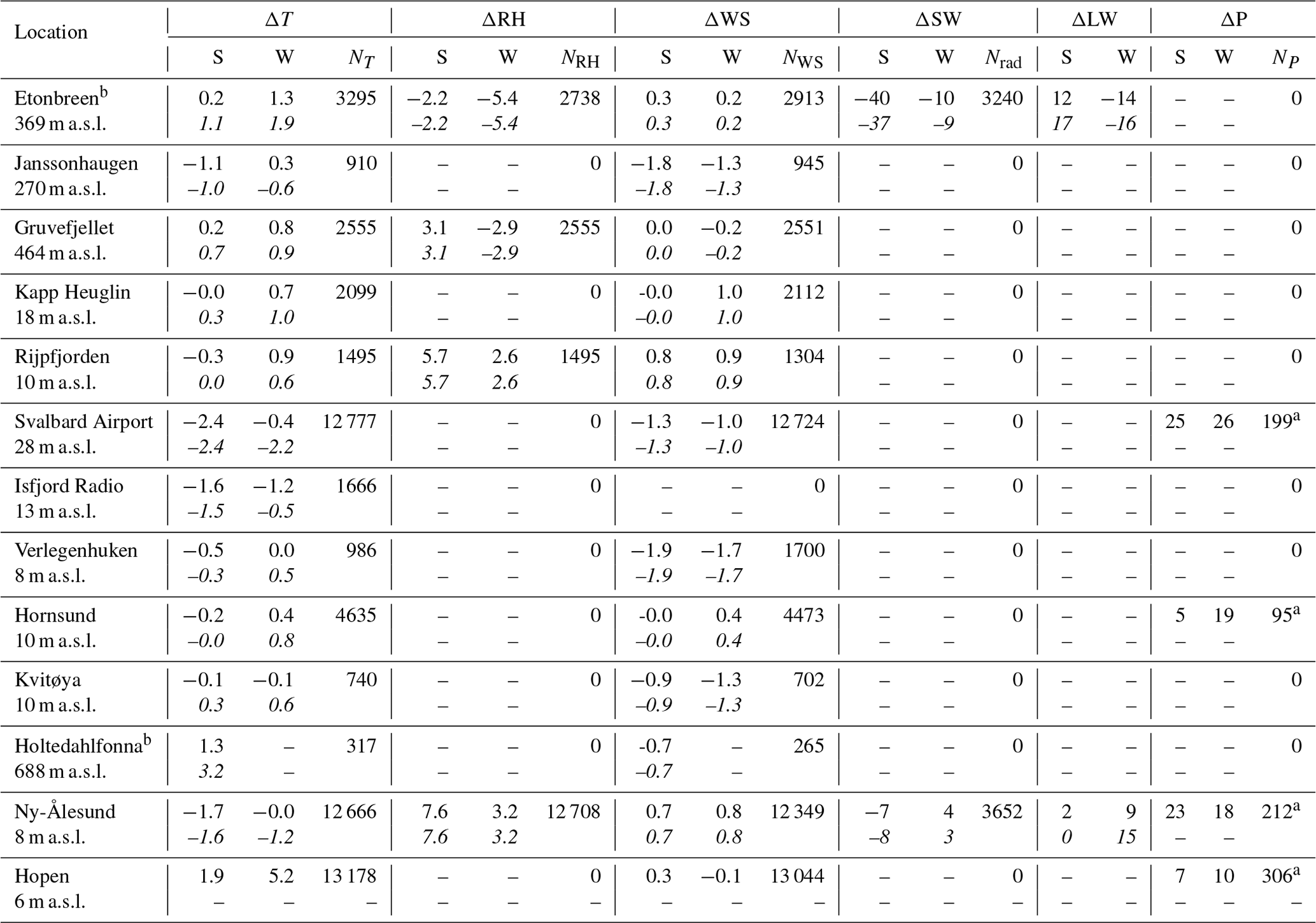
a Number of months. b Station located on a glacier.
3.4 Relative humidity and wind speed
For relative humidity the reanalysis represents the seasonality well, and in late summer both the humidity and the biases are of the largest magnitude. At the two coastal stations at Hopen and Rijpfjorden, the downscaled reanalysis is too dry, whereas it is too humid at the two higher-elevation stations. The coarse land mask of the reanalysis and the poor representation of sea ice are most likely the main causes for these biases. Wind speeds are reproduced reasonably well, including the seasonal cycle (Table 1). Biases are within ±1.5 m s−1 with no clear seasonal trend. It is likely that the biases are caused by site-specific effects, such as deceleration of air flow in the lee of a topographic obstacle or acceleration due to channelizing through valleys.

The downloadable dataset comprises individual files for each of the following variables: precipitation, air temperature, relative humidity, wind speed, and incident shortwave and downwelling longwave radiation. The records are organized as one file per month for each of the reanalysis periods: September 1957 to August 2002 (ERA-40) and January 1979 to December 2017 (ERA-Interim). Each file contains the discovery metadata and the complete metadata to locate the stack of fields in space and time. The grid is regular and rectangular in UTM33X projection, the coordinates of which are defined by the arrays X (meters easting in UTM33X, 448 elements) and Y (meters northing in UTM33X, 548 elements). In geographical coordinates the grid is non-regular, and therefore the location of each grid node is defined, rendering latitude and longitude (in decimal degrees) each as a 448×548 array. The timestamp is given in days since 1 January 1900 using a standard Gregorian calendar of 365 d per year, i.e., without accounting for leap years. In addition, there is one file containing the stationary fields, i.e., the surface topography and land-ocean mask. The file format is netCDF according to the CF conventions (http://cfconventions.org/, last access: 14 April 2020), with all required metadata included. The metadata adhere to ISO19115 geospatial metadata standards and the Directory Interchange Format (DIF) requirements of the Global Change Master Directory GCMD (https://gcmd.nasa.gov/DocumentBuilder/defaultDif10/guide/index.html, last access: 14 April 2020), and global attributes comply to the Attribute Convention for Data Discovery ACDD (http://wiki.esipfed.org/index.php/Attribute_Convention_for_Data_Discovery_1-3, last access: 14 April 2020).
Table 2 gives an overview over the number of files and their sizes for the different epochs (ERA-40, ERA-Interim) and variables contained in the dataset. The naming convention for the individual files is <EPOCH>_<VAR>_<YYYYMM>.nc, where EPOCH is either “ERA40” or “ERAi”, VAR is an abbreviation of the variable of interest (one of “precip”, “temp”, “RH”, “wind speed”, “SWi” or “LWi”) and YYYYMM identifies year and month, e.g., ERAi_temp_200410.nc is the name of the file containing air temperature from ERA-Interim for October 2004.
The dataset is openly available from the National e-Infrastructure for Research Data (NIRD) archive at https://doi.org/10.11582/2018.00006 and referred to as “Svalbard impact assessment forcing dataset, version 1” (Schuler, 2018). Sval_Imp is licensed under the Creative Commons Attribution 4.0 International License (CC-BY 4.0). In essence, you are free to copy, distribute and adapt the work, as long as you attribute the work to its origin and abide by the other license terms.
The MATLAB code used to produce Sval_Imp is available at https://github.com/TVSchuler/Sval_Imp_matlab (Schuler and Østby, 2020) under a GNU GPLv3.0 license.
ERA-40 (Uppala et al., 2005) and ERA-Interim (Dee et al., 2011) data were retrieved from the ECMWF Public Datasets web interface at https://apps.ecmwf.int/datasets/ (ECMWF, 2011).
Weather station data are provided by the Norwegian Meteorological Institute, available at https://seklima.met.no/observations (last access: 14 April 2020), and by the University Centre of Svalbard, available at https://www.unis.no/resources/weather-stations/ (last access: 14 April 2020). Radiation from the Baseline Surface Radiation Network (BRSN) station in Ny-Ålesund are provided by Maturilli et al. (2014).
We present a gridded dataset of near-surface meteorological variables at 1 km resolution covering the Svalbard archipelago. The set of variables enables application of energy balance models and comes at a time steps of 6 h. The high-resolution grids are derived from coarse-scale reanalyses ERA-40 for the period 1957–2002 and from ERA-Interim for 1979–2017. We describe the intermediate-complexity downscaling procedure used to generate this dataset. Furthermore, we evaluate the performance of the downscaled data using a suite of different meteorological and glaciological measurements and refer to several applications of this dataset in different disciplines, all of them requiring long-term coverage at small spatial scales.
TVS retrieved reanalysis data; developed code; and performed the downscaling for precipitation, air temperature, RH, and wind speed. TIØ developed the code and performed downscaling of radiation components. Evaluation performance was conducted collaboratively. TVS was responsible for formatting, providing metadata and archiving the dataset. TVS also led the writing of the manuscript, and TIØ contributed to the writing.
The authors declare that they have no conflict of interest.
We greatly acknowledge the European Centre for Medium-range Weather Forecasts (ECMWF) for giving us access to their reanalysis products ERA-40 and ERA-Interim. The Norwegian Meteorological Institute has been pioneering and is exemplary in providing open access to historical data, especially through their eKlima service. Field work at Austfonna has been supported by NFR through IPY-Glaciodyn, EU-ice2sea and ESA-CRYOVEX. Knut Sand provided access to the Sand et al. (2003) dataset.
This research has been supported by the Nordic Centre of Excellence SVALI, “Stability and Variations of Arctic Land Ice”. The Norwegian Ministry of Education funded a scholarship for Torbjørn Ims Østby.
This paper was edited by Jens Klump and reviewed by Kabir Rasouli and Andrew Newman.
Aalstad, K., Westermann, S., Schuler, T. V., Boike, J., and Bertino, L.: Ensemble-based assimilation of fractional snow-covered area satellite retrievals to estimate the snow distribution at Arctic sites, The Cryosphere, 12, 247–270, https://doi.org/10.5194/tc-12-247-2018, 2018. a
Aas, K. S., Dunse, T., Collier, E., Schuler, T. V., Berntsen, T. K., Kohler, J., and Luks, B.: The climatic mass balance of Svalbard glaciers: a 10-year simulation with a coupled atmosphere–glacier mass balance model, The Cryosphere, 10, 1089–1104, https://doi.org/10.5194/tc-10-1089-2016, 2016. a, b
Barstad, I. and Smith, R. B.: Evaluation of an Orographic Precipitation Model, J. Hydrometeorol., 6, 85–99, https://doi.org/10.1175/JHM-404.1, 2005. a, b
Bogren, W. S., Burkhart, J. F., and Kylling, A.: Tilt error in cryospheric surface radiation measurements at high latitudes: a model study, The Cryosphere, 10, 613–622, https://doi.org/10.5194/tc-10-613-2016, 2016. a
Botnen, S. S.: Biodiversity in the dark: root-associated fungi in the Arctic, PhD-thesis, Department of Biosciences, University of Oslo, Norway, 2020. a
Crochet, P., Jóhannesson, T., Jónsson, T., Sigurðsson, O., Björnsson, H., Pálsson, F., and Barstad, I.: Estimating the Spatial Distribution of Precipitation in Iceland Using a Linear Model of Orographic Precipitation, J. Hydrometeorol., 8, 1285–1306, https://doi.org/10.1175/2007JHM795.1, 2007. a
Dee, D. P., Uppala, S. M., Simmons, A. J., Berrisford, P., Poli, P., Kobayashi, S., Andrae, U., Balmaseda, M. A., Balsamo, G., Bauer, P., Bechtold, P., Beljaars, A. C. M., van de Berg, L., Bidlot, J., Bormann, N., Delsol, C., Dragani, R., Fuentes, M., Geer, A. J., Haimberger, L., Healy, S. B., Hersbach, H., Hólm, E. V., Isaksen, L., Kållberg, P., Köhler, M., Matricardi, M., McNally, A. P., Monge-Sanz, B. M., Morcrette, J.-J., Park, B.-K., Peubey, C., de Rosnay, P., Tavolato, C., Thépaut, J.-N., and Vitart, F.: The ERA-Interim reanalysis: configuration and performance of the data assimilation system, Q. J. Roy. Meteor. Soc., 137, 553–597, https://doi.org/10.1002/qj.828, 2011. a, b
Dunse, T., Schuler, T. V., Hagen, J. O., Eiken, T., Brandt, O., and Høgda, K. A.: Recent fluctuations in the extent of the firn area of Austfonna, Svalbard, inferred from GPR, Ann. Glaciol., 50, 155–162, https://doi.org/10.3189/172756409787769780, 2009. a, b
Ehret, U., Zehe, E., Wulfmeyer, V., Warrach-Sagi, K., and Liebert, J.: HESS Opinions “Should we apply bias correction to global and regional climate model data?”, Hydrol. Earth Syst. Sci., 16, 3391–3404, https://doi.org/10.5194/hess-16-3391-2012, 2012. a
European Centre for Medium-range Weather Forecast (ECMWF) (2011): The ERA-Interim reanalysis dataset, Copernicus Climate Change Service (C3S) available at: https://www.ecmwf.int/en/forecasts/datasets/archive-datasets/reanalysis-datasets/era-interim (last access: 14 April 2020), 2011. a
Fiddes, J. and Gruber, S.: TopoSCALE v.1.0: downscaling gridded climate data in complex terrain, Geosci. Model Dev., 7, 387–405, https://doi.org/10.5194/gmd-7-387-2014, 2014. a, b, c, d, e
Førland, E. J. and Hanssen-Bauer, I.: Increased Precipitation in the Norwegian Arctic: True or False?, Climatic Change, 46, 485–509, https://doi.org/10.1023/A:1005613304674, 2000. a
Grabiec, M., Leszkiewicz, J., Glowacki, P., and Jania, J.: Distribution of snow accumulation on some glaciers of Spitsbergen, Pol. Polar Res., 27, 309–326, 2006. a
Gutmann, E., Barstad, I., Clark, M., Arnold, J., and Rasmussen, R.: The Intermediate Complexity Atmospheric Research Model (ICAR), J. Hydrometeorol., 17, 957–973, https://doi.org/10.1175/JHM-D-15-0155.1, 2016. a
Hanssen-Bauer, I., Førland, E., Hisdal, H., S.Mayer, Sandø, A., Sorteberg, A., Adakudlu, M., Andresen, J., Bakke, J., Beldring, S., Benestad, R., van der Bilt, W., Bogen, J., Borstad, C., Breili, K., Breivik, Ø., Børsheim, K., Christiansen, H., Dobler, A., Engeset, R., Frauenfelder, R., Gerland, S., Gjelten, H., Gundersen, J., Isaksen, K., Jaedicke, C., Kierulf, H., Kohler, J., Li, H., Lutz, J., Melvold, K., Mezghani, A., Nilsen, F., Nilsen, I., Nilsen, J., Pavlova, O., Ravndal, O., Risebrobakken, B., Saloranta, T., Sandven, S., Schuler, T., Simpson, M., Skogen, M., Smedsrud, L., Sund, M., Vikhamar-Schuler, D., Westermann, S., and Wong, W. (Eds.): Climate in Svalbard 2100 – a knowledge base for climate adaptation, vol. 1/2019, Norwegian Environment Agency (Miljødirektoratet), Norwegian Centre for Climate Services, available at: https://cms.met.no/site/2/klimaservicesenteret/climate-in-svalbard-2100/_attachment/14428?_ts=169fd13ff23 (last access: 14 April 2020), 2019. a
Jarosch, A. H., Anslow, F. S., and Clarke, G. K. C.: High-resolution precipitation and temperature downscaling for glacier models, Clim. Dynam., 38, 391–409, https://doi.org/10.1007/s00382-010-0949-1, 2012. a, b
Kumar, L., Skidmore, A., and Knowles, E.: Modelling topographic variation in solar radiation in a GIS environment, Int. J. Geogr. Inf. Sci., 11, 475–497, https://doi.org/10.1080/136588197242266, 1997. a
Liston, G. E. and Elder, K.: A Meteorological Distribution System for High-Resolution Terrestrial Modeling (MicroMet), J. Hydrometeorol., 7, 217–234, https://doi.org/10.1175/JHM486.1, 2006. a
Maraun, D.: Bias Correction, Quantile Mapping, and Downscaling: Revisiting the Inflation Issue, J. Climate, 26, 2137–2143, https://doi.org/10.1175/JCLI-D-12-00821.1, 2013. a
Marshall, S. J., Sharp, M. J., Burgess, D. O., and Anslow, F. S.: Near-surface-temperature lapse rates on the Prince of Wales Icefield, Ellesmere Island, Canada: implications for regional downscaling of temperature, Int. J. Climatol., 27, 385–398, https://doi.org/10.1002/joc.1396, 2007. a
Maturilli, M., Herber, A., and König-Langlo, G.: Basic and other measurements of radiation from the Baseline Surface Radiation Network (BSRN) Station Ny-Ålesund in the years 1992 to 2013, reference list of 253 datasets, PANGAEA, https://doi.org/10.1594/PANGAEA.150000, 2014. a
Maturilli, M., Herber, A.. and König-Langlo, G.: Surface radiation climatology for Ny-Ålesund, Svalbard (78.9∘ N), basic observations for trend detection, Theor. Appl. Climatol., 120, 331–339 https://doi.org/10.1007/s00704-014-1173-4, 2015. a, b, c
Østby, T. I., Schuler, T. V., Hagen, J. O., Hock, R., Kohler, J., and Reijmer, C. H.: Diagnosing the decline in climatic mass balance of glaciers in Svalbard over 1957–2014, The Cryosphere, 11, 191–215, https://doi.org/10.5194/tc-11-191-2017, 2017. a, b, c, d, e, f, g
Pramanik, A., Van Pelt, W., Kohler, J., and Schuler, T.: Simulating climatic mass balance, seasonal snow development and associated freshwater runoff in the Kongsfjord basin, Svalbard (1980–2016), J. Glaciol., 64, 943–956, https://doi.org/10.1017/jog.2018.80, 2018. a
Ratti, C.: Urban analysis for environmental prediction, PhD thesis, University of Cambridge Department of Architecture, 2001. a
Reda, I. and Andreas, A.: Solar position algorithm for solar radiation applications, Sol. Energy, 76, 577–589, https://doi.org/10.1016/j.solener.2003.12.003, 2004. a
Roth, A., Hock, R., Schuler, T. V., Bieniek, P. A., Pelto, M., and Aschwanden, A.: Modeling Winter Precipitation Over the Juneau Icefield, Alaska, Using a Linear Model of Orographic Precipitation, Front. Earth Sci., 6, 20 pp., https://doi.org/10.3389/feart.2018.00020, 2018. a
Sand, K., Winther, J.-G., Maréchal, D., Bruland, O., and Melvold, K.: Regional Variations of Snow Accumulation on Spitsbergen, Svalbard, 1997–99, Hydrol. Res., 34, 17–32, https://doi.org/10.2166/nh.2003.0026, 2003. a
Schuler, T.: Svalbard impact assessment forcing dataset, version 1, [Data set], Norstore, https://doi.org/10.11582/2018.00006, 2018. a, b, c, d
Schuler, T. V. and Østby, T. I.: Sval_Imp-matlab: First release of Sval_imp-matlab, Zenodo, https://doi.org/10.5281/zenodo.3719367, 2020. a
Schuler, T., Dunse, T., Østby, T., and Hagen, J.: Meteorological conditions on an Arctic ice cap–8 years of automatic weather station data from Austfonna, Svalbard, Int. J. Climatol., 34, 2047–2058, https://doi.org/10.1002/joc.3821, 2014. a
Schuler, T. V., Loe, E., Taurisano, A., Eiken, T., Hagen, J. O., and Kohler, J.: Calibrating a surface mass-balance model for Austfonna ice cap, Svalbard, Ann. Glaciol., 46, 241–248, https://doi.org/10.3189/172756407782871783, 2007. a
Schuler, T. V., Crochet, P., Hock, R., Jackson, M., Barstad, I., and Jóhannesson, T.: Distribution of snow accumulation on the Svartisen ice cap, Norway, assessed by a model of orographic precipitation, Hydrol. Process., 22, 3998–4008, https://doi.org/10.1002/hyp.7073, 2008. a, b, c
Sinclair, M. R.: A Diagnostic Model for Estimating Orographic Precipitation, J. Appl. Meteorol., 33, 1163–1175, https://doi.org/10.1175/1520-0450(1994)033<1163:ADMFEO>2.0.CO;2, 1994. a
Smith, R. B. and Barstad, I.: A Linear Theory of Orographic Precipitation, J. Atmos. Sci., 61, 1377–1391, https://doi.org/10.1175/1520-0469(2004)061<1377:ALTOOP>2.0.CO;2, 2004. a, b, c
Stone, P. H. and Carlson, J. H.: Atmospheric Lapse Rate Regimes and Their Parameterization, J. Atmos. Sci., 36, 415–423, 1979. a
Taurisano, A., Schuler, T. V., Hagen, J. O., Eiken, T., Loe, E., Melvold, K., and Kohler, J.: The distribution of snow accumulation across the Austfonna ice cap, Svalbard: direct measurements and modelling, Polar Res., 26, 7–13, https://doi.org/10.1111/j.1751-8369.2007.00004.x, 2007. a, b
Uppala, S. M., KÅllberg, P. W., Simmons, A. J., Andrae, U., Bechtold, V. D. C., Fiorino, M., Gibson, J. K., Haseler, J., Hernandez, A., Kelly, G. A., Li, X., Onogi, K., Saarinen, S., Sokka, N., Allan, R. P., Andersson, E., Arpe, K., Balmaseda, M. A., Beljaars, A. C. M., Berg, L. V. D., Bidlot, J., Bormann, N., Caires, S., Chevallier, F., Dethof, A., Dragosavac, M., Fisher, M., Fuentes, M., Hagemann, S., Hólm, E., Hoskins, B. J., Isaksen, L., Janssen, P. A. E. M., Jenne, R., Mcnally, A. P., Mahfouf, J.-F., Morcrette, J.-J., Rayner, N. A., Saunders, R. W., Simon, P., Sterl, A., Trenberth, K. E., Untch, A., Vasiljevic, D., Viterbo, P., and Woollen, J.: The ERA-40 re-analysis, Q. J. Roy. Meteor. Soc., 131, 2961–3012, https://doi.org/10.1256/qj.04.176, 2005. a, b
Vikhamar-Schuler, D., Førland, E., Lutz, J., and Gjelten, H.: Evaluation of downscaled reanalysis and observations for Svalbard: Background report for Climate in Svalbard 2100, Tech. rep., Norwegian Centre for Climate Services, 2019. a, b, c
Wolff, M. A., Isaksen, K., Petersen-Øverleir, A., Ødemark, K., Reitan, T., and Brækkan, R.: Derivation of a new continuous adjustment function for correcting wind-induced loss of solid precipitation: results of a Norwegian field study, Hydrol. Earth Syst. Sci., 19, 951–967, https://doi.org/10.5194/hess-19-951-2015, 2015. a