the Creative Commons Attribution 4.0 License.
the Creative Commons Attribution 4.0 License.
 | 05 Dec 2018
Global Carbon Budget 2018
Corinne Le Quéré
Robbie M. Andrew
Pierre Friedlingstein
Stephen Sitch
Judith Hauck
Julia Pongratz
Penelope A. Pickers
Jan Ivar Korsbakken
Glen P. Peters
Josep G. Canadell
Almut Arneth
Vivek K. Arora
Leticia Barbero
Ana Bastos
Laurent Bopp
Frédéric Chevallier
Louise P. Chini
Philippe Ciais
Scott C. Doney
Thanos Gkritzalis
Daniel S. Goll
Ian Harris
Vanessa Haverd
Forrest M. Hoffman
Mario Hoppema
Richard A. Houghton
George Hurtt
Tatiana Ilyina
Atul K. Jain
Truls Johannessen
Chris D. Jones
Etsushi Kato
Ralph F. Keeling
Kees Klein Goldewijk
Peter Landschützer
Nathalie Lefèvre
Sebastian Lienert
Danica Lombardozzi
Nicolas Metzl
David R. Munro
Julia E. M. S. Nabel
Shin-ichiro Nakaoka
Craig Neill
Are Olsen
Tsueno Ono
Prabir Patra
Anna Peregon
Wouter Peters
Philippe Peylin
Benjamin Pfeil
Denis Pierrot
Benjamin Poulter
Gregor Rehder
Laure Resplandy
Eddy Robertson
Matthias Rocher
Christian Rödenbeck
Ute Schuster
Jörg Schwinger
Roland Séférian
Ingunn Skjelvan
Tobias Steinhoff
Adrienne Sutton
Pieter P. Tans
Hanqin Tian
Bronte Tilbrook
Francesco N. Tubiello
Ingrid T. van der Laan-Luijkx
Guido R. van der Werf
Nicolas Viovy
Anthony P. Walker
Andrew J. Wiltshire
Rebecca Wright
Sönke Zaehle
Accurate assessment of anthropogenic carbon dioxide (CO2) emissions and their redistribution among the atmosphere, ocean, and terrestrial biosphere – the “global carbon budget” – is important to better understand the global carbon cycle, support the development of climate policies, and project future climate change. Here we describe data sets and methodology to quantify the five major components of the global carbon budget and their uncertainties. Fossil CO2 emissions (EFF) are based on energy statistics and cement production data, while emissions from land use and land-use change (ELUC), mainly deforestation, are based on land use and land-use change data and bookkeeping models. Atmospheric CO2 concentration is measured directly and its growth rate (GATM) is computed from the annual changes in concentration. The ocean CO2 sink (SOCEAN) and terrestrial CO2 sink (SLAND) are estimated with global process models constrained by observations. The resulting carbon budget imbalance (BIM), the difference between the estimated total emissions and the estimated changes in the atmosphere, ocean, and terrestrial biosphere, is a measure of imperfect data and understanding of the contemporary carbon cycle. All uncertainties are reported as ±1σ. For the last decade available (2008–2017), EFF was 9.4±0.5 GtC yr−1, ELUC 1.5±0.7 GtC yr−1, GATM 4.7±0.02 GtC yr−1, SOCEAN 2.4±0.5 GtC yr−1, and SLAND 3.2±0.8 GtC yr−1, with a budget imbalance BIM of 0.5 GtC yr−1 indicating overestimated emissions and/or underestimated sinks. For the year 2017 alone, the growth in EFF was about 1.6 % and emissions increased to 9.9±0.5 GtC yr−1. Also for 2017, ELUC was 1.4±0.7 GtC yr−1, GATM was 4.6±0.2 GtC yr−1, SOCEAN was 2.5±0.5 GtC yr−1, and SLAND was 3.8±0.8 GtC yr−1, with a BIM of 0.3 GtC. The global atmospheric CO2 concentration reached 405.0±0.1 ppm averaged over 2017. For 2018, preliminary data for the first 6–9 months indicate a renewed growth in EFF of +2.7 % (range of 1.8 % to 3.7 %) based on national emission projections for China, the US, the EU, and India and projections of gross domestic product corrected for recent changes in the carbon intensity of the economy for the rest of the world. The analysis presented here shows that the mean and trend in the five components of the global carbon budget are consistently estimated over the period of 1959–2017, but discrepancies of up to 1 GtC yr−1 persist for the representation of semi-decadal variability in CO2 fluxes. A detailed comparison among individual estimates and the introduction of a broad range of observations show (1) no consensus in the mean and trend in land-use change emissions, (2) a persistent low agreement among the different methods on the magnitude of the land CO2 flux in the northern extra-tropics, and (3) an apparent underestimation of the CO2 variability by ocean models, originating outside the tropics. This living data update documents changes in the methods and data sets used in this new global carbon budget and the progress in understanding the global carbon cycle compared with previous publications of this data set (Le Quéré et al., 2018, 2016, 2015a, b, 2014, 2013). All results presented here can be downloaded from https://doi.org/10.18160/GCP-2018.


The concentration of carbon dioxide (CO2) in the atmosphere has increased from approximately 277 parts per million (ppm) in 1750 (Joos and Spahni, 2008), the beginning of the industrial era, to 405.0±0.1 ppm in 2017 (Dlugokencky and Tans, 2018; Fig. 1). The atmospheric CO2 increase above pre-industrial levels was, initially, primarily caused by the release of carbon to the atmosphere from deforestation and other land-use change activities (Ciais et al., 2013). While emissions from fossil fuels started before the industrial era, they only became the dominant source of anthropogenic emissions to the atmosphere around 1950 and their relative share has continued to increase until present. Anthropogenic emissions occur on top of an active natural carbon cycle that circulates carbon among the reservoirs of the atmosphere, ocean, and terrestrial biosphere on timescales from sub-daily to millennial, while exchanges with geologic reservoirs occur at longer timescales (Archer et al., 2009).
The global carbon budget presented here refers to the mean, variations, and trends in the perturbation of CO2 in the environment, referenced to the beginning of the industrial era. It quantifies the input of CO2 to the atmosphere by emissions from human activities, the growth rate of atmospheric CO2 concentration, and the resulting changes in the storage of carbon in the land and ocean reservoirs in response to increasing atmospheric CO2 levels, climate change, and variability and other anthropogenic and natural changes (Fig. 2). An understanding of this perturbation budget over time and the underlying variability and trends in the natural carbon cycle is necessary to understand the response of natural sinks to changes in climate, CO2 and land-use change drivers, and the permissible emissions for a given climate stabilisation target.
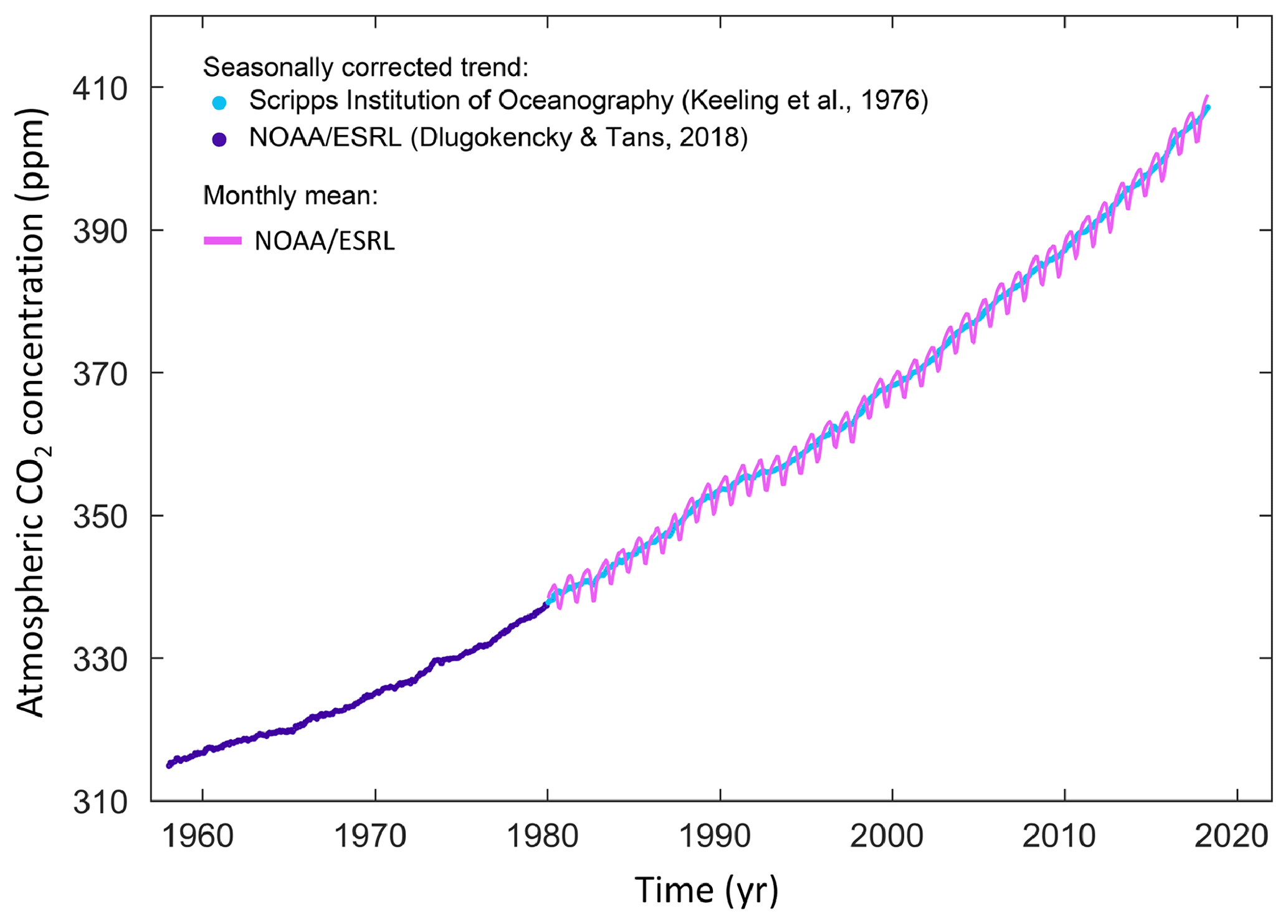
Figure 1Surface average atmospheric CO2 concentration (ppm). The 1980–2018 monthly data are from NOAA/ESRL (Dlugokencky and Tans, 2018) and are based on an average of direct atmospheric CO2 measurements from multiple stations in the marine boundary layer (Masarie and Tans, 1995). The 1958–1979 monthly data are from the Scripps Institution of Oceanography, based on an average of direct atmospheric CO2 measurements from the Mauna Loa and South Pole stations (Keeling et al., 1976). To take into account the difference of mean CO2 and seasonality between the NOAA/ESRL and the Scripps station networks used here, the Scripps surface average (from two stations) was deseasonalised and harmonised to match the NOAA/ESRL surface average (from multiple stations) by adding the mean difference of 0.542 ppm, calculated here from overlapping data during 1980–2012.
The components of the CO2 budget that are reported annually in this paper include separate estimates for (1) the CO2 emissions from fossil fuel combustion and oxidation from all energy and industrial processes and cement production (EFF; GtC yr−1); (2) the emissions resulting from deliberate human activities on land, including those leading to land-use change (ELUC; GtC yr−1); and (3) their partitioning among the growth rate of atmospheric CO2 concentration (GATM; GtC yr−1), the uptake of CO2 (the “CO2 sinks”) in (4) the ocean (SOCEAN; GtC yr−1), and (5) the uptake of CO2 on land (SLAND; GtC yr−1). The CO2 sinks as defined here conceptually include the response of the land (including inland waters and estuaries) and ocean (including coasts and territorial sea) to elevated CO2 and changes in climate, rivers, and other environmental conditions, although in practice not all processes are accounted for (see Sect. 2.8). The global emissions and their partitioning among the atmosphere, ocean, and land are in reality in balance; however due to imperfect spatial and/or temporal data coverage, errors in each estimate, and smaller terms not included in our budget estimate (discussed in Sect. 2.8), their sum does not necessarily add up to zero. We estimate a budget imbalance (BIM), which is a measure of the mismatch between the estimated emissions and the estimated changes in the atmosphere, land, and ocean, with the full global carbon budget as follows:
GATM is usually reported in ppm yr−1, which we convert to units of carbon mass per year, GtC yr−1, using 1 ppm =2.124 GtC (Table 1). We also include a quantification of EFF by country, computed with both territorial and consumption-based accounting (see Sect. 2), and discuss missing terms from sources other than the combustion of fossil fuels (see Sect. 2.8).
Table 1Factors used to convert carbon in various units (by convention, Unit 1 = Unit 2 conversion).
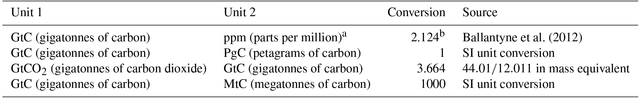
a Measurements of atmospheric CO2 concentration have units of dry-air mole fraction. “ppm” is an abbreviation for micromole mol−1, dry air. b The use of a factor of 2.124 assumes that all the atmosphere is well mixed within 1 year. In reality, only the troposphere is well mixed and the growth rate of CO2 concentration in the less well-mixed stratosphere is not measured by sites from the NOAA network. Using a factor of 2.124 makes the approximation that the growth rate of CO2 concentration in the stratosphere equals that of the troposphere on a yearly basis.
The CO2 budget has been assessed by the Intergovernmental Panel on Climate Change (IPCC) in all assessment reports (Ciais et al., 2013; Denman et al., 2007; Prentice et al., 2001; Schimel et al., 1995; Watson et al., 1990), and by others (e.g. Ballantyne et al., 2012). The IPCC methodology has been adapted and used by the Global Carbon Project (GCP, http://www.globalcarbonproject.org/, last access: 30 November 2018), which has coordinated a cooperative community effort for the annual publication of global carbon budgets up to the year 2005 (Raupach et al., 2007; including fossil emissions only), the year 2006 (Canadell et al., 2007), the year 2007 (published online; GCP, 2007), the year 2008 (Le Quéré et al., 2009), the year 2009 (Friedlingstein et al., 2010), the year 2010 (Peters et al., 2012b), the year 2012 (Le Quéré et al., 2013; Peters et al., 2013), the year 2013 (Le Quéré et al., 2014), the year 2014 (Friedlingstein et al., 2014; Le Quéré et al., 2015b), the year 2015 (Jackson et al., 2016; Le Quéré et al., 2015a), the year 2016 (Le Quéré et al., 2016), and most recently the year 2017 (Le Quéré et al., 2018; Peters et al., 2017). Each of these papers updated previous estimates with the latest available information for the entire time series.
We adopt a range of ±1 standard deviation (σ) to report the uncertainties in our estimates, representing a likelihood of 68 % that the true value will be within the provided range if the errors have a Gaussian distribution and no bias is assumed. This choice reflects the difficulty of characterising the uncertainty in the CO2 fluxes between the atmosphere and the ocean and land reservoirs individually, particularly on an annual basis, as well as the difficulty of updating the CO2 emissions from land use and land-use change. A likelihood of 68 % provides an indication of our current capability to quantify each term and its uncertainty given the available information. For comparison, the Fifth Assessment Report of the IPCC (AR5) generally reported a likelihood of 90 % for large data sets whose uncertainty is well characterised or for long time intervals less affected by year-to-year variability. Our 68 % uncertainty value is near the 66 % which the IPCC characterises as “likely” for values falling into the ±1σ interval. The uncertainties reported here combine statistical analysis of the underlying data and expert judgement of the likelihood of results lying outside this range. The limitations of current information are discussed in the paper and have been examined in detail elsewhere (Ballantyne et al., 2015; Zscheischler et al., 2017). We also use a qualitative assessment of confidence level to characterise the annual estimates from each term based on the type, amount, quality, and consistency of the evidence as defined by the IPCC (Stocker et al., 2013).
All quantities are presented in units of gigatonnes of carbon (GtC, 1015 gC), which is the same as petagrams of carbon (PgC; Table 1). Units of gigatonnes of CO2 (or billion tonnes of CO2) used in policy are equal to 3.664 multiplied by the value in units of GtC.
This paper provides a detailed description of the data sets and methodology used to compute the global carbon budget estimates for the pre-industrial period (1750) to 2017 and in more detail for the period since 1959. It also provides decadal averages starting in 1960 including the last decade (2008–2017), results for the year 2017, and a projection for the year 2018. Finally it provides cumulative emissions from fossil fuels and land-use change since the year 1750, the pre-industrial period, and since the year 1870, the reference year for the cumulative carbon estimate used by the IPCC (AR5) based on the availability of global temperature data (Stocker et al., 2013). This paper is updated every year using the format of “living data” to keep a record of budget versions and the changes in new data, revision of data, and changes in methodology that lead to changes in estimates of the carbon budget. Additional materials associated with the release of each new version will be posted at the Global Carbon Project (GCP) website (http://www.globalcarbonproject.org/carbonbudget, last access: 30 November 2018), with fossil fuel emissions also available through the Global Carbon Atlas (http://www.globalcarbonatlas.org, last access: 30 November 2018). With this approach, we aim to provide the highest transparency and traceability in the reporting of CO2, the key driver of climate change.
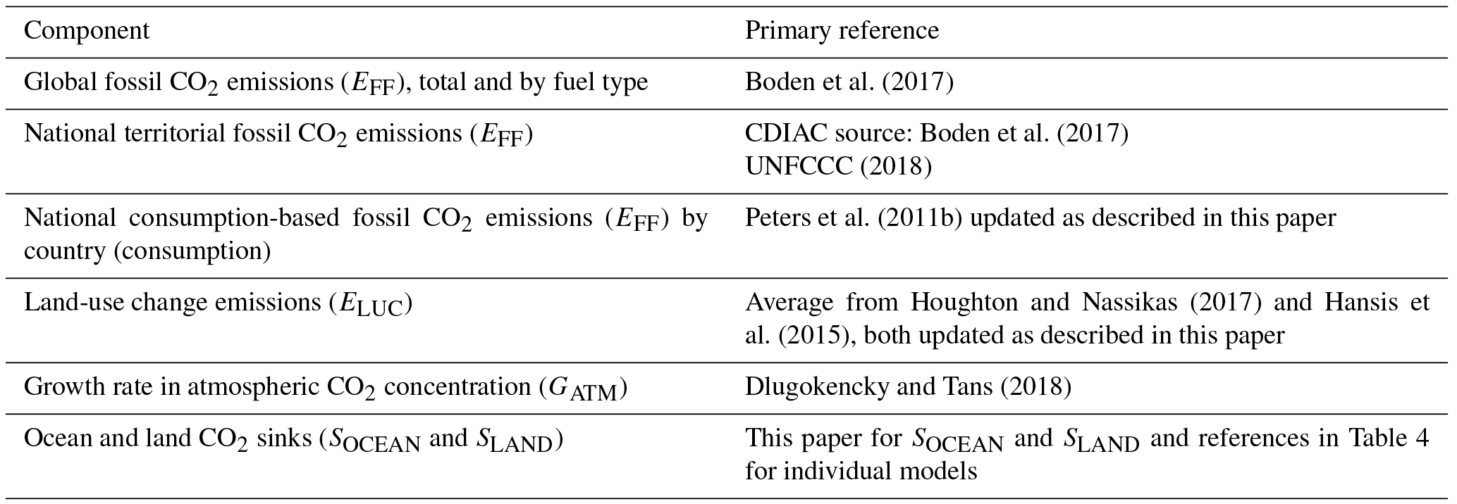
Multiple organisations and research groups around the world generated the original measurements and data used to complete the global carbon budget. The effort presented here is thus mainly one of synthesis, in which results from individual groups are collated, analysed, and evaluated for consistency. We facilitate access to original data with the understanding that primary data sets will be referenced in future work (see Table 2 for how to cite the data sets). Descriptions of the measurements, models, and methodologies follow below and in depth descriptions of each component are described elsewhere.
Table 2How to cite the individual components of the global carbon budget presented here.
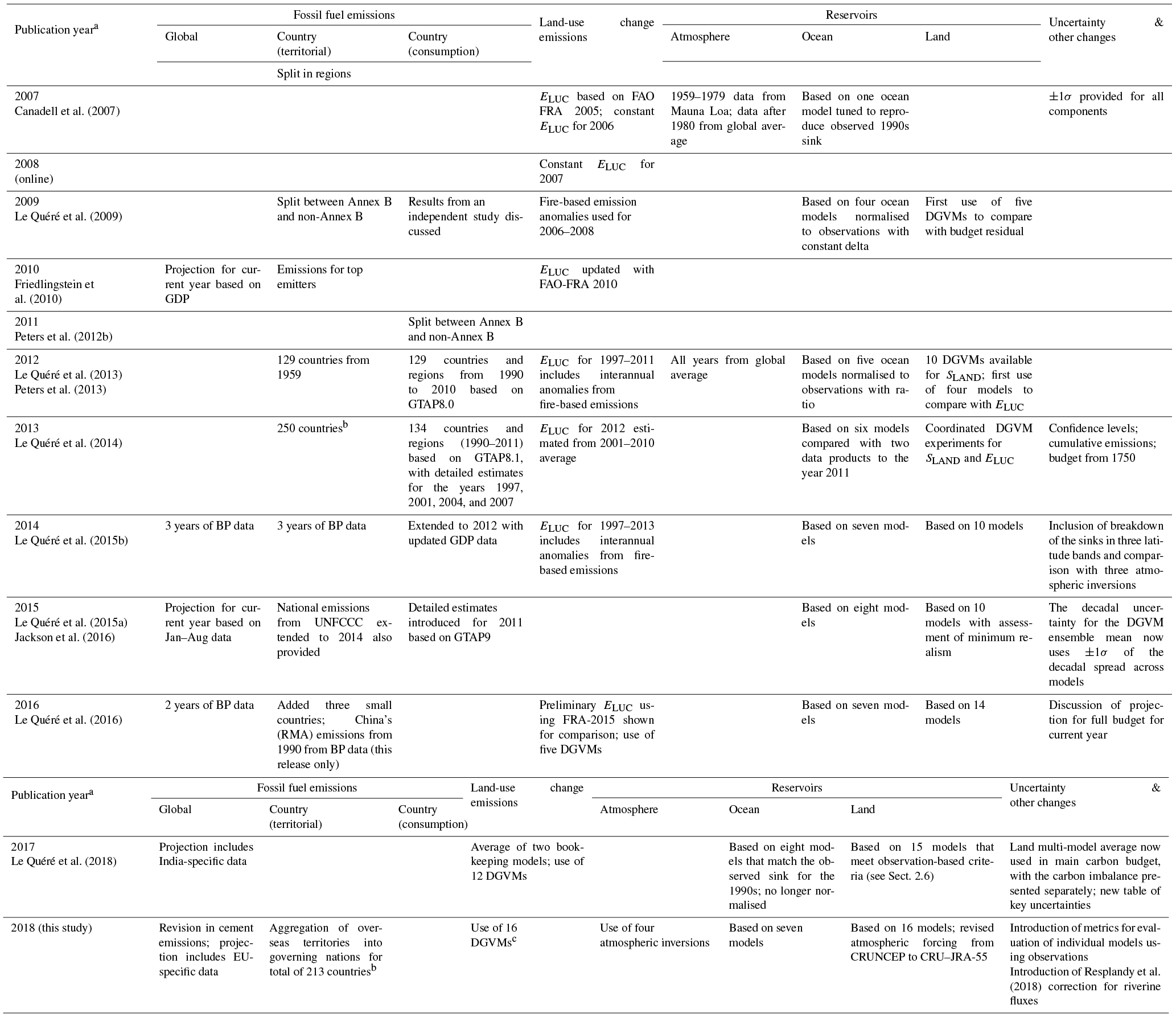
This is the 13th version of the global carbon budget and the seventh revised version in the format of a living data update. It builds on the latest published global carbon budget of Le Quéré et al. (2018). The main changes are (1) the inclusion of data to the year 2017 (inclusive) and a projection for the global carbon budget for the year 2018; (2) the introduction of metrics that evaluate components of the individual models used to estimate SOCEAN and SLAND using observations, as an effort to document, encourage, and support model improvements through time; (3) the revisions of the CO2 emissions associated with cement production based on revised clinker ratios; (4) a projection for fossil fuel emissions for the 28 European Union member states based on compiled energy statistics; and (5) the addition of Sect. 2.8.2 on additional emissions from calcination not included in the budget. The main methodological differences among annual carbon budgets are summarised in Table 3.
Table 3Main methodological changes in the global carbon budget since first publication. Methodological changes introduced in one year are kept for the following years unless noted. Empty cells mean there were no methodological changes introduced that year.
2.1 Fossil CO2 emissions (EFF)
2.1.1 Emission estimates
The estimates of global and national fossil CO2 emissions (EFF) include the combustion of fossil fuels through a wide range of activities (e.g. transport, heating, and cooling, industry, fossil industry's own use, and gas flaring), the production of cement, and other process emissions (e.g. the production of chemicals and fertilisers). The estimates of EFF rely primarily on energy consumption data, specifically data on hydrocarbon fuels, collated and archived by several organisations (Andres et al., 2012). We use four main data sets for historical emissions (1751–2017).
-
We use global and national emission estimates for coal, oil, and gas from CDIAC for the time period of 1751–2014 (Boden et al., 2017), as it is the only data set that extends back to 1751 by country.
-
We use official UNFCCC national inventory reports for 1990–2016 for the 42 Annex I countries in the UNFCCC (UNFCCC, 2018). We assess these to be the most accurate estimates because they are compiled by experts within countries that have access to detailed energy data, and they are periodically reviewed.
-
We use the BP Statistical Review of World Energy (BP, 2018), as these are the most up-to-date estimates of national energy statistics.
-
We use global and national cement emissions updated from Andrew (2018), which include revised emission factors.
In the following section we provide more details for each data set and describe the additional modifications that are required to make the data set consistent and usable.
-
CDIAC. The CDIAC estimates have been updated annually to the year 2014, derived primarily from energy statistics published by the United Nations (UN, 2017b). Fuel masses and volumes are converted to fuel energy content using country-level coefficients provided by the UN and then converted to CO2 emissions using conversion factors that take into account the relationship between carbon content and energy (heat) content of the different fuel types (coal, oil, gas, gas flaring) and the combustion efficiency (Marland and Rotty, 1984).
-
UNFCCC. Estimates from the UNFCCC national inventory reports follow the IPCC guidelines (IPCC, 2006) but have a slightly larger system boundary than CDIAC by including emissions coming from carbonates other than in cement manufacturing. We reallocate the detailed UNFCCC estimates to the CDIAC definitions of coal, oil, gas, cement, and other to allow consistent comparisons over time and among countries.
-
BP. For the most recent period when the UNFCCC (2018) and CDIAC (2015–2017) estimates are not available, we generate preliminary estimates using the BP Statistical Review of World Energy (Andres et al., 2014; Myhre et al., 2009; BP, 2018). We apply the BP growth rates by fuel type (coal, oil, gas) to estimate 2017 emissions based on 2016 estimates (UNFCCC) and to estimate 2015–2017 emissions based on 2014 estimates (CDIAC). BP's data set explicitly covers about 70 countries (96 % of global emissions), and for the remaining countries we use growth rates from the subregion the country belongs to. For the most recent years, flaring is assumed constant from the most recent available year of data (2016 for countries that report to the UNFCCC, 2014 for the remainder).
-
Cement. Estimates of emissions from cement production are taken directly from Andrew (2018). Additional calcination and carbonation processes are not included explicitly here, except in national inventories provided by UNFCCC, but are discussed in Sect. 2.8.2.
-
Country mappings. The published CDIAC data set includes 256 countries and regions. This list includes countries that no longer exist, such as the USSR and Yugoslavia. We reduce the list to 213 countries by reallocating emissions to the currently defined territories, using mass-preserving aggregation or disaggregation. Examples of aggregation include merging East and West Germany to the currently defined Germany. Examples of disaggregation include reallocating the emissions from the former USSR to the resulting independent countries. For disaggregation, we use the emission shares when the current territories first appeared, and thus historical estimates of disaggregated countries should be treated with extreme care. In addition, we aggregate some overseas territories (e.g. Réunion, Guadeloupe) into their governing nations (e.g. France) to align with UNFCCC reporting.
-
Global total. Our global estimate is based on CDIAC for fossil fuel combustion plus Andrew (2018) for cement emissions. This is greater than the sum of emissions from all countries. This is largely attributable to emissions that occur in international territory, in particular, the combustion of fuels used in international shipping and aviation (bunker fuels). The emissions from international bunker fuels are calculated based on where the fuels were loaded, but we do not include them in the national emission estimates. Other differences occur (1) because the sum of imports in all countries is not equal to the sum of exports, and (2) because of inconsistent national reporting, differing treatment of oxidation of non-fuel uses of hydrocarbons (e.g. as solvents, lubricants, feedstocks), and (3) because of changes in fuel stored (Andres et al., 2012).
2.2 Uncertainty assessment for EFF
We estimate the uncertainty of the global fossil CO2 emissions at ±5 % (scaled down from the published ±10 % at ±2σ to the use of ±1σ bounds reported here; Andres et al., 2012). This is consistent with a more detailed recent analysis of uncertainty of ±8.4 % at ±2σ (Andres et al., 2014) and at the high end of the range of ±5–10 % at ±2σ reported by Ballantyne et al. (2015). This includes an assessment of uncertainties in the amounts of fuel consumed, the carbon and heat contents of fuels, and the combustion efficiency. While we consider a fixed uncertainty of ±5 % for all years, the uncertainty as a percentage of the emissions is growing with time because of the larger share of global emissions from emerging economies and developing countries (Marland et al., 2009). Generally, emissions from mature economies with good statistical processes have an uncertainty of only a few per cent (Marland, 2008), while emissions from developing countries such as China have uncertainties of around ±10 % (for ±1σ; Gregg et al., 2008). Uncertainties of emissions are likely to be mainly systematic errors related to underlying biases of energy statistics and to the accounting method used by each country.
We assign a medium confidence to the results presented here because they are based on indirect estimates of emissions using energy data (Durant et al., 2011). There is only limited and indirect evidence for emissions, although there is high agreement among the available estimates within the given uncertainty (Andres et al., 2012, 2014), and emission estimates are consistent with a range of other observations (Ciais et al., 2013), even though their regional and national partitioning is more uncertain (Francey et al., 2013).
2.2.1 Emissions embodied in goods and services
CDIAC, UNFCCC, and BP national emission statistics “include greenhouse gas emissions and removals taking place within national territory and offshore areas over which the country has jurisdiction” (Rypdal et al., 2006) and are called territorial emission inventories. Consumption-based emission inventories allocate emissions to products that are consumed within a country and are conceptually calculated as the territorial emissions minus the “embodied” territorial emissions to produce exported products plus the emissions in other countries to produce imported products (consumption = territorial − exports + imports). Consumption-based emission attribution results (e.g. Davis and Caldeira, 2010) provide additional information to territorial-based emissions that can be used to understand emission drivers (Hertwich and Peters, 2009) and quantify emission transfers by the trade of products between countries (Peters et al., 2011b). The consumption-based emissions have the same global total but reflect the trade-driven movement of emissions across the Earth's surface in response to human activities.
We estimate consumption-based emissions from 1990 to 2016 by enumerating the global supply chain using a global model of the economic relationships between economic sectors within and among every country (Andrew and Peters, 2013; Peters et al., 2011a). Our analysis is based on the economic and trade data from the Global Trade and Analysis Project (GTAP; Narayanan et al., 2015), and we make detailed estimates for the years 1997 (GTAP version 5), 2001 (GTAP6), and 2004, 2007, and 2011 (GTAP9.2), covering 57 sectors and 141 countries and regions. The detailed results are then extended into an annual time series from 1990 to the latest year of the gross domestic product (GDP) data (2016 in this budget), using GDP data by expenditure in the current exchange rate of US dollars (USD; from the UN National Accounts Main Aggregrates Database; UN, 2017a) and time series of trade data from GTAP (based on the methodology in Peters et al., 2011b). We estimate the sector-level CO2 emissions using the GTAP data and methodology, include flaring and cement emissions from CDIAC, and then scale the national totals (excluding bunker fuels) to match the emission estimates from the carbon budget. We do not provide a separate uncertainty estimate for the consumption-based emissions, but based on model comparisons and sensitivity analysis, they are unlikely to be significantly different than for the territorial emission estimates (Peters et al., 2012a).
2.2.2 Growth rate in emissions
We report the annual growth rate in emissions for adjacent years (in per cent per year) by calculating the difference between the two years and then normalising to the emissions in the first year: . . We apply a leap-year adjustment when relevant to ensure valid interpretations of annual growth rates. This affects the growth rate by about 0.3 % yr−1 (1∕365) and causes growth rates to go up approximately 0.3 % if the first year is a leap year and down 0.3 % if the second year is a leap year.
The relative growth rate of EFF over time periods of greater than 1 year can be rewritten using its logarithm equivalent as follows:
Here we calculate relative growth rates in emissions for multi-year periods (e.g. a decade) by fitting a linear trend to ln(EFF) in Eq. (2), reported in per cent per year.
2.2.3 Emission projections
To gain insight into emission trends for the current year (2018), we provide an assessment of global fossil CO2 emissions, EFF, by combining individual assessments of emissions for China, the US, the EU, and India (the four countries/regions with the largest emissions), and the rest of the world.
Our 2018 estimate for China uses (1) the sum of domestic production (NBS, 2018b) and net imports (General Administration of Customs of the People's Republic of China, 2018) for coal, oil and natural gas, and production of cement (NBS, 2018b) from preliminary statistics for January through September of 2018 and (2) historical relationships between January–September statistics for both production and imports and full-year statistics for consumption using final data for 2000–2016 (NBS, 2015, 2017) and preliminary data for 2017 (NBS, 2018a). See also Liu et al. (2018) and Jackson et al. (2018) for details. The uncertainty is based on the variance of the difference between the January–September and full-year data from historical data, as well as typical variance in the preliminary full-year data used for 2017 and typical changes in the energy content of coal for the period of 2013–2016 (NBS, 2017, 2015). We note that developments for the final 3 months this year may be atypical due to the ongoing trade disputes between China and the US, and this additional uncertainty has not been quantified. Results and uncertainties are discussed further in Sect. 3.4.1.
For the US, we use the forecast of the U.S. Energy Information Administration (EIA) for emissions from fossil fuels (EIA, 2018). This is based on an energy forecasting model which is updated monthly (last update to October) and takes into account heating-degree days, household expenditures by fuel type, energy markets, policies, and other effects. We combine this with our estimate of emissions from cement production using the monthly US cement data from the U.S. Geological Survey (USGS) for January–August, assuming changes in cement production over the first part of the year apply throughout the year. While the EIA's forecasts for current full-year emissions have on average been revised downwards, only 10 such forecasts are available, so we conservatively use the full range of adjustments following revision and additionally assume symmetrical uncertainty to give ±2.5 % around the central forecast.
For India, we use (1) monthly coal production and sales data from the Ministry of Mines (2018), Coal India Limited (CIL, 2018), and Singareni Collieries Company Limited (SCCL, 2018), combined with import data from the Ministry of Commerce and Industry (MCI, 2018) and power station stocks data from the Central Electricity Authority (CEA, 2018); (2) monthly oil production and consumption data from the Ministry of Petroleum and Natural Gas (PPAC, 2018a); (3) monthly natural gas production and import data from the Ministry of Petroleum and Natural Gas (PPAC, 2018b); and (4) monthly cement production data from the Office of the Economic Advisor (OEA, 2018). All data were available for January to September or October. We use Holt–Winters exponential smoothing with multiplicative seasonality (Chatfield, 1978) on each of these four emission series to project to the end of the current year. This iterative method produces estimates of both trend and seasonality at the end of the observation period that are a function of all prior observations, weighted most strongly to more recent data, while maintaining some smoothing effect. The main source of uncertainty in the projection of India's emissions is the assumption of continued trends and typical seasonality.
For the EU, we use (1) monthly coal supply data from Eurostat for the first 6–9 months of the year (Eurostat, 2018) cross-checked with more recent data on coal-generated electricity from ENTSO-E for January through October (ENTSO-E, 2018); (2) monthly oil and gas demand data for January through August from the Joint Organisations Data Initiative (JODI, 2018); and (3) cement production assumed to be stable. For oil and gas emissions we apply the Holt–Winters method separately to each country and energy carrier to project to the end of the current year, while for coal – which is much less strongly seasonal because of strong weather variations – we assume the remaining months of the year are the same as the previous year in each country.
For the rest of the world, we use the close relationship between the growth in GDP and the growth in emissions (Raupach et al., 2007) to project emissions for the current year. This is based on a simplified Kaya identity, whereby EFF (GtC yr−1) is decomposed by the product of GDP (USD yr−1) and the fossil fuel carbon intensity of the economy (IFF; GtC USD−1) as follows:
Taking a time derivative of Eq. (3) and rearranging gives
where the left-hand term is the relative growth rate of EFF, and the right-hand terms are the relative growth rates of GDP and IFF, respectively, which can simply be added linearly to give the overall growth rate.
The growth rates are reported in per cent by multiplying each term by 100. As preliminary estimates of annual change in GDP are made well before the end of a calendar year, making assumptions on the growth rate of IFF allows us to make projections of the annual change in CO2 emissions well before the end of a calendar year. The IFF is based on GDP in constant PPP (purchasing power parity) from the International Energy Agency (IEA) up until 2016 (IEA/OECD, 2017) and extended using the International Monetary Fund (IMF) growth rates for 2016 and 2017 (IMF, 2018). Interannual variability in IFF is the largest source of uncertainty in the GDP-based emission projections. We thus use the standard deviation of the annual IFF for the period of 2007–2017 as a measure of uncertainty, reflecting a ±1σ as in the rest of the carbon budget. This is ±1.0 % yr−1 for the rest of the world (global emissions minus China, the US, the EU, and India).
The 2018 projection for the world is made of the sum of the projections for China, the US, the EU, India, and the rest of the world. The uncertainty is added in quadrature among the five regions. The uncertainty here reflects the best of our expert opinion.
2.3 CO2 emissions from land use, land-use change, and forestry (ELUC)
The net CO2 flux from land use, land-use change, and forestry (ELUC, called land-use change emissions in the rest of the text) include CO2 fluxes from deforestation, afforestation, logging and forest degradation (including harvest activity), shifting cultivation (cycle of cutting forest for agriculture, then abandoning), and regrowth of forests following wood harvest or abandonment of agriculture. Only some land management activities are included in our land-use change emission estimates (Table A1 in the Appendix). Some of these activities lead to emissions of CO2 to the atmosphere, while others lead to CO2 sinks. ELUC is the net sum of emissions and removals due to all anthropogenic activities considered. Our annual estimate for 1959–2017 is provided as the average of results from two bookkeeping models (Sect. 2.3.1): the estimate published by Houghton and Nassikas (2017; hereafter H&N2017) extended here to 2017 and an estimate using the BLUE model (Bookkeeping of Land Use Emissions; Hansis et al., 2015). In addition, we use results from dynamic global vegetation models (DGVMs; see Sect. 2.3.3 and Table 4) to help quantify the uncertainty in ELUC and thus better characterise our understanding. The three methods are described below, and differences are discussed in Sect. 3.2.
Table 4References for the process models, pCO2-based ocean flux products, and atmospheric inversions included in Figs. 6–8. All models and products are updated with new data to the end of the year 2017, and the atmospheric forcing for the DGVMs has been updated as described in Sect. 2.3.2.
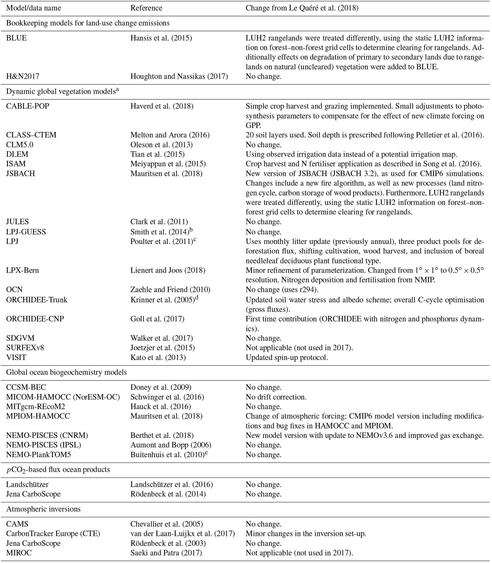
a The forcing for all DGVMs has been updated from CRUNCEP to CRU–JRA. b To account for the differences between the derivation of shortwave radiation (SWRAD) from CRU cloudiness and SWRAD from CRU–JRA-55, the photosynthesis scaling parameter αa was modified (−15 %) to yield similar results. c Compared to the published version, LPJ wood harvest efficiency was decreased so that 50 % of biomass was removed off-site compared to 85 % used in the 2012 budget. Residue management of managed grasslands increased so that 100 % of harvested grass enters the litter pool. d Compared to the published version, new hydrology and snow scheme; revised parameter values for photosynthetic capacity for all ecosystem (following assimilation of FLUXNET data), updated parameters values for stem allocation, maintenance respiration, and biomass export for tropical forests (based on literature), and CO2 down-regulation process added to photosynthesis. Version used for CMIP6. e No nutrient restoring below the mixed-layer depth.
2.3.1 Bookkeeping models
Land-use change CO2 emissions and uptake fluxes are calculated by two bookkeeping models. Both are based on the original bookkeeping approach of Houghton (2003) that keeps track of the carbon stored in vegetation and soils before and after a land-use change (transitions between various natural vegetation types, croplands, and pastures). Literature-based response curves describe decay of vegetation and soil carbon, including transfer to product pools of different lifetimes, as well as carbon uptake due to regrowth. In addition, the bookkeeping models represent long-term degradation of primary forest as lowered standing vegetation and soil carbon stocks in secondary forests and also include forest management practices such as wood harvests.
The bookkeeping models do not include land ecosystems' transient response to changes in climate, atmospheric CO2, and other environmental factors, and the carbon densities are based on contemporary data reflecting environmental conditions at (and up to) that time. Since carbon densities remain fixed over time in bookkeeping models, the additional sink capacity that ecosystems provide in response to CO2 fertilisation and some other environmental changes is not captured by these models (Pongratz et al., 2014; see Sect. 2.8.4).
The H&N2017 and BLUE models differ in (1) computational units (country level vs. spatially explicit treatment of land-use change), (2) processes represented (see Table A1), and (3) carbon densities assigned to vegetation and soil of each vegetation type. A notable change of H&N2017 over the original approach by Houghton et al. (2003) used in earlier budget estimates is that no shifting cultivation or other back-and-forth transitions below the country level are included. Only a decline in forest area in a country as indicated by the Forest Resource Assessment of the FAO that exceeds the expansion of agricultural area as indicated by the FAO is assumed to represent a concurrent expansion and abandonment of cropland. In contrast, the BLUE model includes sub-grid-scale transitions at the grid level among all vegetation types as indicated by the harmonised land-use change data (LUH2) data set (https://doi.org/10.22033/ESGF/input4MIPs.1127; Hurtt et al., 2011, 2018). Furthermore, H&N2017 assume conversion of natural grasslands to pasture, while BLUE allocates pasture proportionally on all natural vegetation that exists in a grid cell. This is one reason for generally higher emissions in BLUE. H&N2017 add carbon emissions from peat burning based on the Global Fire Emission Database (GFED4s; van der Werf et al., 2017) and peat drainage based on estimates by Hooijer et al. (2010) to the output of their bookkeeping model for the countries of Indonesia and Malaysia. Peat burning and emissions from the organic layers of drained peat soils, which are not captured by bookkeeping methods directly, need to be included to represent the substantially larger emissions and interannual variability due to synergies of land use and climate variability in Southeast Asia, in particular during El Niño events. Similarly to H&N2017, peat burning and drainage-related emissions are also added to the BLUE estimate.
The two bookkeeping estimates used in this study also differ with respect to the land-use change data used to drive the models. H&N2017 base their estimates directly on the Forest Resource Assessment of the FAO, which provides statistics on forest area change and management at intervals of 5 years currently updated until 2015 (FAO, 2015). The data are based on country reporting to the FAO and may include remote-sensing information in more recent assessments. Changes in land use other than forests are based on annual national changes in cropland and pasture areas reported by the FAO (FAOSTAT, 2015). BLUE uses the harmonised land-use change data LUH2 (https://doi.org/10.22033/ESGF/input4MIPs.1127, Hurtt et al., 2011, 2018), which describe land-use change, also based on the FAO data, but downscaled at a quarter-degree spatial resolution, considering sub-grid-scale transitions among primary forest, secondary forest, cropland, pasture, and rangeland. The LUH2 data provide a new distinction between rangelands and pasture. To constrain the models' interpretation on whether rangeland implies the original natural vegetation to be transformed to grassland or not (e.g. browsing on shrubland), a new forest mask was provided with LUH2; forest is assumed to be transformed, while all other natural vegetation remains. This is implemented in BLUE.
The estimate of H&N2017 was extended here by 2 years (to 2017) by adding the anomaly of total tropical emissions (peat drainage from Hooijer et al. (2010), peat burning, and tropical deforestation and degradation fires (from GFED4s) over the previous decade (2006–2015) to the decadal average of the bookkeeping result.
2.3.2 Dynamic global vegetation models (DGVMs)
Land-use change CO2 emissions have also been estimated using an ensemble of 16 DGVM simulations. The DGVMs account for deforestation and regrowth, the most important components of ELUC, but they do not represent all processes resulting directly from human activities on land (Table A1). All DGVMs represent processes of vegetation growth and mortality, as well as decomposition of dead organic matter associated with natural cycles, and include the vegetation and soil carbon response to increasing atmospheric CO2 levels and to climate variability and change. Some models explicitly simulate the coupling of carbon and nitrogen cycles and account for atmospheric N deposition (Table A1). The DGVMs are independent from the other budget terms except for their use of atmospheric CO2 concentration to calculate the fertilisation effect of CO2 on plant photosynthesis.
The DGVMs used the HYDE land-use change data set (Klein Goldewijk et al., 2017a, b), which provides annual half-degree fractional data on cropland and pasture. These data are based on annual FAO statistics of change in agricultural land area available until 2012. The FAOSTAT land use database is updated annually, currently covering the period of 1961–2016 (but used here until 2015 because of the timing of data availability). HYDE-applied annual changes in FAO data to the year 2012 from the previous release are used to derive new 2013–2015 data. After the year 2015 HYDE extrapolates cropland, pasture, and urban land use data until the year 2018. Some models also use an update of the more comprehensive harmonised land-use data set (Hurtt et al., 2011), which further includes fractional data on primary and secondary forest vegetation, as well as all underlying transitions between land-use states (Hurtt et al., 2018; Table A1). This new data set is of quarter-degree fractional areas of land use states and all transitions between those states, including a new wood harvest reconstruction, new representation of shifting cultivation, crop rotations, and management information including irrigation and fertiliser application. The land-use states now include five different crop types in addition to the pasture–rangeland split discussed before. Wood harvest patterns are constrained with Landsat tree cover loss data.
DGVMs implement land-use change differently (e.g. an increased cropland fraction in a grid cell can be at the expense of either grassland or shrubs, or forest, the latter resulting in deforestation; land cover fractions of the non-agricultural land differ among models). Similarly, model-specific assumptions are applied to convert deforested biomass or deforested area and other forest product pools into carbon, and different choices are made regarding the allocation of rangelands as natural vegetation or pastures.
The DGVM model runs were forced by either the merged monthly CRU and 6-hourly JRA-55 data set or by the monthly CRU data set, both providing observation-based temperature, precipitation, and incoming surface radiation on a grid and updated to 2017 (Harris et al., 2014). The combination of CRU monthly data with 6-hourly forcing is updated this year from NCEP to JRA-55 (Kobayashi et al., 2015), adapting the methodology used in previous years (Viovy, 2016) to the specifics of the JRA-55 data. The forcing data also include global atmospheric CO2, which changes over time (Dlugokencky and Tans, 2018) and gridded time-dependent N deposition (as used in some models; Table A1).
Two sets of simulations were performed with the DGVMs. Both applied historical changes in climate, atmospheric CO2 concentration, and N deposition. The two sets of simulations differ, however, with respect to land use: one set applies historical changes in land use, the other a time-invariant pre-industrial land cover distribution and pre-industrial wood harvest rates. By difference of the two simulations, the dynamic evolution of vegetation biomass and soil carbon pools in response to land use change can be quantified in each model (ELUC). We only retain model outputs with positive ELUC, i.e. a positive flux to the atmosphere, during the 1990s (Table A1). Using the difference between these two DGVM simulations to diagnose ELUC means the DGVMs account for the loss of additional sink capacity (around 0.3 GtC yr−1; see Sect. 2.8.4), while the bookkeeping models do not.
2.3.3 Uncertainty assessment for ELUC
Differences between the bookkeeping models and DGVM models originate from three main sources: the different methodologies, the underlying land use/land cover data set, and the different processes represented (Table A1). We examine the results from the DGVM models and from the bookkeeping method and use the resulting variations as a way to characterise the uncertainty in ELUC.
Table 5Comparison of results from the bookkeeping method and budget residuals with results from the DGVMs and inverse estimates for different periods, the last decade, and the last year available. All values are in GtC yr−1. The DGVM uncertainties represent ±1σ of the decadal or annual (for 2017 only) estimates from the individual DGVMs: for the inverse models the range of available results is given.
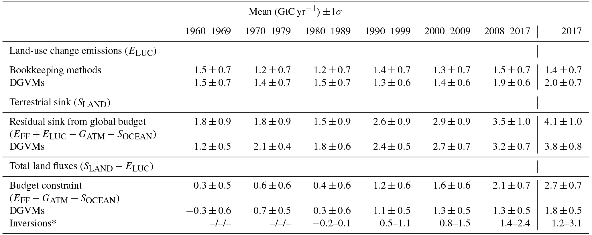
* Estimates are corrected for the pre-industrial influence of river fluxes
and adjusted to common EFF (Sect. 2.8.2). Two inversions are
available for the 1980s and 1990s.
Two additional inversions are available
from 2001 and used from the decade of the 2000s (Table A3).
The ELUC estimate from the DGVMs multi-model mean is consistent with the average of the emissions from the bookkeeping models (Table 5). However there are large differences among individual DGVMs (standard deviation at around 0.6–0.7 GtC yr−1; Table 5), between the two bookkeeping models (average of 0.7 GtC yr−1), and between the current estimate of H&N2017 and its previous model version (Houghton et al., 2012). The uncertainty in ELUC of ±0.7 GtC yr−1 reflects our best value judgment that there is at least a 68 % chance (±1σ) that the true land-use change emission lies within the given range, for the range of processes considered here. Prior to the year 1959, the uncertainty in ELUC was taken from the standard deviation of the DGVMs. We assign low confidence to the annual estimates of ELUC because of the inconsistencies among estimates and of the difficulties to quantify some of the processes in DGVMs.
2.3.4 Emission projections
We project emissions for both H&N2017 and BLUE for 2018 using the same approach as for the extrapolation of H&N2017 for 2016–2017. Peat burning as well as tropical deforestation and degradation are estimated using active fire data (MCD14ML; Giglio et al., 2016), which scales almost linearly with GFED (van der Werf et al., 2017) and thus allows for tracking fire emissions in deforestation and tropical peat zones in near-real time. During most years, emissions during January–October cover most of the fire season in the Amazon and Southeast Asia, where a large part of the global deforestation takes place.
2.4 Growth rate in atmospheric CO2 concentration (GATM)
2.4.1 Global growth rate in atmospheric CO2 concentration
The rate of growth of the atmospheric CO2 concentration is provided by the US National Oceanic and Atmospheric Administration Earth System Research Laboratory (NOAA/ESRL, 2018; Dlugokencky and Tans, 2018), which is updated from Ballantyne et al. (2012). For the 1959–1979 period, the global growth rate is based on measurements of atmospheric CO2 concentration averaged from the Mauna Loa and South Pole stations, as observed by the CO2 Program at the Scripps Institution of Oceanography (Keeling et al., 1976). For the 1980–2017 time period, the global growth rate is based on the average of multiple stations selected from the marine boundary layer sites with well-mixed background air (Ballantyne et al., 2012), after fitting each station with a smoothed curve as a function of time and averaging by latitude band (Masarie and Tans, 1995). The annual growth rate is estimated by Dlugokencky and Tans (2018) from the atmospheric CO2 concentration by taking the average of the most recent December–January months corrected for the average seasonal cycle and subtracting this same average 1 year earlier. The growth rate in units of ppm yr−1 is converted to units of GtC yr−1 by multiplying by a factor of 2.124 GtC per ppm (Ballantyne et al., 2012).
The uncertainty around the atmospheric growth rate is due to four main factors. The first factor is the long-term reproducibility of reference gas standards (around 0.03 ppm for 1σ from the 1980s). The second factor is that small unexplained systematic analytical errors that may have a duration of several months to 2 years come and go. They have been simulated by randomising both the duration and the magnitude (determined from the existing evidence) in a Monte Carlo procedure. The third factor is the network composition of the marine boundary layer with some sites coming or going, gaps in the time series at each site, etc. (Dlugokencky and Tans, 2018). The latter uncertainty was estimated by NOAA/ESRL with a Monte Carlo method by constructing 100 “alternative” networks (NOAA/ESRL, 2018; Masarie and Tans, 1995). The second and third uncertainties, summed in quadrature, add up to 0.085 ppm on average (Dlugokencky and Tans, 2018). Fourth, the uncertainty associated with using the average CO2 concentration from a surface network to approximate the true atmospheric average CO2 concentration (mass weighted, in three dimensions) as needed to assess the total atmospheric CO2 burden. In reality, CO2 variations measured at the stations will not exactly track changes in total atmospheric burden, with offsets in magnitude and phasing due to vertical and horizontal mixing. This effect must be very small on decadal and longer timescales, when the atmosphere can be considered well mixed. Preliminary estimates suggest this effect would increase the annual uncertainty, but a full analysis is not yet available. We therefore maintain an uncertainty around the annual growth rate based on the multiple stations' data set ranges between 0.11 and 0.72 GtC yr−1, with a mean of 0.61 GtC yr−1 for 1959–1979 and 0.18 GtC yr−1 for 1980–2017, when a larger set of stations were available as provided by Dlugokencky and Tans (2018), but recognise further exploration of this uncertainty is required. At this time, we estimate the uncertainty of the decadal averaged growth rate after 1980 at 0.02 GtC yr−1 based on the calibration and the annual growth rate uncertainty, but stretched over a 10-year interval. For years prior to 1980, we estimate the decadal averaged uncertainty to be 0.07 GtC yr−1 based on a factor proportional to the annual uncertainty prior to and after 1980 ( GtC yr−1).
We assign a high confidence to the annual estimates of GATM because they are based on direct measurements from multiple and consistent instruments and stations distributed around the world (Ballantyne et al., 2012).
In order to estimate the total carbon accumulated in the atmosphere since 1750 or 1870, we use an atmospheric CO2 concentration of 277±3 ppm or 288±3 ppm, respectively, based on a cubic spline fit to ice core data (Joos and Spahni, 2008). The uncertainty of ±3 ppm (converted to ±1σ) is taken directly from the IPCC's assessment (Ciais et al., 2013). Typical uncertainties in the growth rate in atmospheric CO2 concentration from ice core data are equivalent to ±0.1–0.15 GtC yr−1 as evaluated from the Law Dome data (Etheridge et al., 1996) for individual 20-year intervals over the period from 1870 to 1960 (Bruno and Joos, 1997).
2.4.2 Atmospheric growth rate projection
We provide an assessment of GATM for 2018 based on the observed increase in atmospheric CO2 concentration at the Mauna Loa station for January to October and a mean growth rate over the past 5 years for the months November to December. Growth at Mauna Loa is closely correlated with the global growth (r=0.95) and is used here as a proxy for global growth, but the regression is not 1 to 1. We also adjust the projected global growth rate to take this into account. The assessment method used this year differs from the forecast method used in Le Quéré et al. (2018) based on the relationship between annual CO2 growth rate and sea surface temperatures (SSTs) in the Niño3.4 region of Betts et al. (2016). A change was introduced because although the observed growth rate for 2017 of 2.2 ppm was within the projection range of 2.5±0.5 ppm of last year ( Le Quéré et al., 2018), the forecast values for 2018 for January to October are too high by approximately 0.4 ppm above observed values on average. The reasons for the difference are being investigated. The use of observed growth at Mauna Loa Observatory, Hawaii, for the first half of the year is thought to be more robust because of its high correlation with the global growth rate. Furthermore, additional analysis suggests that the first half of the year shows more interannual variability than the second half of the year, so that the exact projection method applied to November–December has only a small impact (<0.1 ppm) on the projection of the full year. Uncertainty is estimated from past variability using the standard deviation of the last 5 years' monthly growth rates.
2.5 Ocean CO2 sink
Estimates of the global ocean CO2 sink SOCEAN are from an ensemble of global ocean biogeochemistry models (GOBMs) that meet observational constraints over the 1990s (see below). We use observation-based estimates of SOCEAN to provide a qualitative assessment of confidence in the reported results and to estimate the cumulative accumulation of SOCEAN over the pre-industrial period.
2.5.1 Observation-based estimates
We use the observational constraints assessed by IPCC of a mean ocean CO2 sink of 2.2±0.4 GtC yr−1 for the 1990s (Denman et al., 2007) to verify that the GOBMs provide a realistic assessment of SOCEAN. This is based on indirect observations with seven different methodologies and their uncertainties, using the methods that are deemed most reliable for the assessment of this quantity (Denman et al., 2007). The IPCC confirmed this assessment in 2013 (Ciais et al., 2013). The observational-based estimates use the ocean–land CO2 sink partitioning from observed atmospheric O2∕N2 concentration trends (Manning and Keeling, 2006; updated in Keeling and Manning 2014), an oceanic inversion method constrained by ocean biogeochemistry data (Mikaloff Fletcher et al., 2006), and a method based on a penetration timescale for chlorofluorocarbons (McNeil et al., 2003). The IPCC estimate of 2.2 GtC yr−1 for the 1990s is consistent with a range of methods (Wanninkhof et al., 2013).
We also use two estimates of the ocean CO2 sink and its variability based on interpolations of measurements of surface ocean fugacity of CO2 (pCO2 corrected for the non-ideal behaviour of the gas; Pfeil et al., 2013). We refer to these as pCO2-based flux estimates. The measurements are from the Surface Ocean CO2 Atlas version 6, which is an update of version 3 (Bakker et al., 2016) and contains quality-controlled data until 2017 (see data attribution Table A4). The SOCAT v6 data were mapped using a data-driven diagnostic method (Rödenbeck et al., 2013) and a combined self-organising map and feed-forward neural network (Landschützer et al., 2014). The global pCO2-based flux estimates were adjusted to remove the pre-industrial ocean source of CO2 to the atmosphere of 0.78 GtC yr−1 from river input to the ocean (Resplandy et al., 2018), per our definition of SOCEAN. Several other ocean sink products based on observations are also available but they continue to show large unresolved discrepancies with observed variability. Here we used the two pCO2-based flux products that had the best fit to observations for their representation of tropical and global variability (Rödenbeck et al., 2015).
We further use results from two diagnostic ocean models of Khatiwala et al. (2013) and DeVries (2014) to estimate the anthropogenic carbon accumulated in the ocean prior to 1959. The two approaches assume constant ocean circulation and biological fluxes, with SOCEAN estimated as a response in the change in atmospheric CO2 concentration calibrated to observations. The uncertainty in cumulative uptake of ±20 GtC (converted to ±1σ) is taken directly from the IPCC's review of the literature (Rhein et al., 2013), or about ±30 % for the annual values (Khatiwala et al., 2009).
2.5.2 Global ocean biogeochemistry models (GOBMs)
The ocean CO2 sink for 1959–2017 is estimated using seven GOBMs (Table A2). The GOBMs represent the physical, chemical, and biological processes that influence the surface ocean concentration of CO2 and thus the air–sea CO2 flux. The GOBMs are forced by meteorological reanalysis and atmospheric CO2 concentration data available for the entire time period. They mostly differ in the source of the atmospheric forcing data (meteorological reanalysis), spin-up strategies, and their horizontal and vertical resolutions (Table A2). GOBMs do not include the effects of anthropogenic changes in nutrient supply, which could lead to an increase in the ocean sink of up to about 0.3 GtC yr−1 over the industrial period (Duce et al., 2008). They also do not include the perturbation associated with changes in riverine organic carbon (see Sect. 2.8.3).
2.5.3 GOBM evaluation and uncertainty assessment for SOCEAN
The mean ocean CO2 sink for all GOBMs falls within 90 % confidence of the observed range, or 1.6 to 2.8 GtC yr−1 for the 1990s. Here we have adjusted the confidence interval to the IPCC confidence interval of 90 % to avoid rejecting models that may be outliers but are still plausible.
The GOBMs and flux products have been further evaluated using fCO2 from the SOCAT v6 database. We focused this initial evaluation on the interannual mismatch metric proposed by Rödenbeck et al. (2015) for the comparison of flux products. The metric provides a measure of the mismatch between observations and models or flux products on the x axis as well as a measure of the amplitude of the interannual variability on the y axis. A smaller number on the x axis indicates a better fit with observations. The amplitude of the interannual variability in SOCEAN (y axis) is calculated as the temporal standard deviation of the CO2 flux time series.
The calculation for the x axis is carried out as follows: (1) the mismatch between the observed and the modelled fCO2 is calculated for the period 1985 to 2017 (except for the IPSL model, which uses 1985 to 2015 due to data availability), but only for grid points for which actual observations exist. (2) The interannual variability in this mismatch is calculated as the temporal standard deviation of the mismatch. (3) To put numbers into perspective, the interannual variability in the mismatch is reported relative to the interannual variability in the mismatch between a benchmark fCO2 field and the observations. The benchmark fCO2 field is designed to have no interannual variability, i.e. it is calculated as the mean seasonal cycle at each grid point over the full period plus the deseasonalised atmospheric fCO2 increase over time. By definition, the interannual variability in the misfit between benchmark and observations is large as the benchmark field does not contain any interannual variability from the ocean. A smaller relative interannual variability mismatch indicates a better fit between observed and modelled fCO2. This metric is chosen because it is the most direct measure of the year-to-year variability in SOCEAN in ocean biogeochemistry models. We apply the metric globally and by latitude bands. Results are shown in Fig. B1 and discussed in Sect. 3.1.3.
The uncertainty around the mean ocean sink of anthropogenic CO2 was quantified by Denman et al. (2007) for the 1990s (see Sect. 2.5.1). To quantify the uncertainty around annual values, we examine the standard deviation of the GOBM ensemble, which averages between 0.2 and 0.3 GtC yr−1 during 1959–2017. We estimate that the uncertainty in the annual ocean CO2 sink is about ±0.5 GtC yr−1 from the combined uncertainty of the mean flux based on observations of ±0.4 GtC yr−1 and the standard deviation across GOBMs of up to ±0.3 GtC yr−1, reflecting the uncertainty in both the mean sink from observations during the 1990s (Denman et al., 2007; Sect. 2.5.1) and the interannual variability as assessed by GOBMs.
We examine the consistency between the variability in the model-based and the pCO2-based flux products to assess confidence in SOCEAN. The interannual variability in the ocean fluxes (quantified as the standard deviation) of the two pCO2-based flux products for 1985–2017 (where they overlap) is ±0.36 GtC yr−1 (Rödenbeck et al., 2014) and ±0.38 GtC yr−1 (Landschützer et al., 2015), compared to ±0.29 GtC yr−1 for the GOBM ensemble. The standard deviation includes a component of trend and decadal variability in addition to interannual variability, and their relative influence differs across estimates. Individual estimates (both GOBM and flux products) generally produce a higher ocean CO2 sink during strong El Niño events. The annual pCO2-based flux products correlate with the ocean CO2 sink estimated here with a correlation of r=0.75 (0.59 to 0.79 for individual GOBMs) and r=0.80 (0.71 to 0.81) for the pCO2-based flux products of Rödenbeck et al. (2014) and Landschützer et al. (2015), respectively (simple linear regression), with their mutual correlation at 0.73. The agreement between models and the flux products reflects some consistency in their representation of underlying variability since there is little overlap in their methodology or use of observations. The use of annual data for the correlation may reduce the strength of the relationship because the dominant source of variability associated with El Niño events is less than 1 year. We assess a medium confidence level to the annual ocean CO2 sink and its uncertainty because it is based on multiple lines of evidence, and the results are consistent in that the interannual variability in the GOBMs and data-based estimates are all generally small compared to the variability in the growth rate of atmospheric CO2 concentration.
2.6 Terrestrial CO2 sink
2.6.1 DGVM simulations
The terrestrial land sink (SLAND) is thought to be due to the combined effects of fertilisation by rising atmospheric CO2 and N deposition on plant growth, as well as the effects of climate change such as the lengthening of the growing season in northern temperate and boreal areas. SLAND does not include land sinks directly resulting from land use and land-use change (e.g. regrowth of vegetation) as these are part of the land use flux (ELUC), although system boundaries make it difficult to exactly attribute CO2 fluxes on land between SLAND and ELUC (Erb et al., 2013).
SLAND is estimated from the multi-model mean of the DGVMs (Table 4). As described in Sect. 2.3.2, DGVM simulations include all climate variability and CO2 effects over land, with some DGVMs also including the effect of N deposition. The DGVMs do not include the perturbation associated with changes in river organic carbon, which is discussed in Sect. 2.8.
2.6.2 DGVM evaluation and uncertainty assessment for SLAND
We apply three criteria for minimum DGVM realism by including only those DGVMs with (1) steady state after spin-up; (2) net land fluxes (SLAND–ELUC) that are the atmosphere-to-land carbon flux over the 1990s ranging between −0.3 and 2.3 GtC yr−1, within 90 % confidence of constraints by global atmospheric and oceanic observations (Keeling and Manning, 2014; Wanninkhof et al., 2013); and (3) global ELUC that is a carbon source to the atmosphere over the 1990s. All 16 DGVMs meet the three criteria.
In addition, the DGVM results are now also evaluated using the International Land Model Benchmarking System (ILAMB; Collier et al., 2018). This evaluation is provided here to document, encourage, and support model improvements through time. ILAMB variables cover key processes that are relevant for the quantification of SLAND and resulting aggregated outcomes. The selected variables are vegetation biomass, gross primary productivity, leaf area index, net ecosystem exchange, ecosystem respiration, evapotranspiration, and runoff (see Fig. B2 for the results and for the list of observed databases). Results are shown in Fig. B2 and discussed in Sect. 3.1.3.
For the uncertainty, we use the standard deviation of the annual CO2 sink across the DGVMs, which averages to ±0.8 GtC yr−1 for the period from 1959 to 2017. We attach a medium confidence level to the annual land CO2 sink and its uncertainty because the estimates from the residual budget and averaged DGVMs match well within their respective uncertainties (Table 5).
2.7 The atmospheric perspective
The worldwide network of atmospheric measurements can be used with atmospheric inversion methods to constrain the location of the combined total surface CO2 fluxes from all sources, including fossil and land-use change emissions and land and ocean CO2 fluxes. The inversions assume EFF to be well known, and they solve for the spatial and temporal distribution of land and ocean fluxes from the residual gradients of CO2 among stations that are not explained by fossil fuel emissions.
Four atmospheric inversions (Table A3) used atmospheric CO2 data until the end of 2017 (including preliminary values in some cases) to infer the spatio-temporal distribution of the CO2 flux exchanged between the atmosphere and the land or oceans. We focus here on the largest and most consistent sources of information, namely the total land and ocean CO2 fluxes and their partitioning among the mid- to high-latitude region of the Northern Hemisphere (30–90∘ N), the tropics (30∘ S–30∘ N), and the mid- to high-latitude region of the Southern Hemisphere (30–90∘ S). We also break down those estimates for the land and ocean regions separately, to further scrutinise the constraints from atmospheric observations. We use these estimates to comment on the consistency across various data streams and process-based estimates.
2.7.1 Atmospheric inversions
The four inversion systems used in this release are CarbonTracker Europe (CTE; van der Laan-Luijkx et al., 2017), Jena CarboScope (Rödenbeck, 2005), the Copernicus Atmosphere Monitoring Service (CAMS; Chevallier et al., 2005), and MIROC (Patra et al., 2018). See Table A3 for version numbers. The inversions are based on the same Bayesian inversion principles that interpret the same, for the most part, observed time series (or subsets thereof) but use different methodologies (Table A3). These differences mainly concern the selection of atmospheric CO2 data, the used prior fluxes, spatial breakdown (i.e. grid size), assumed correlation structures, and mathematical approach. The details of these approaches are documented extensively in the references provided above. Each system uses a different transport model, which was demonstrated to be a driving factor behind differences in atmospheric-based flux estimates, and specifically their distribution across latitudinal bands (e.g. Gaubert et al., 2018).
The inversions use atmospheric CO2 observations from various flask and in situ networks, as detailed in Table A3. They prescribe global EFF, which is scaled to the present study for CAMS and CTE, while slightly lower EFF values based on alternative emission compilations were used in CarboScope and MIROC. Since this is known to result directly in lower total CO2 uptake in atmospheric inversions (Gaubert et al., 2018; Peylin et al., 2013), we adjusted the land sink of each inversion estimate (where most of the emissions occur) by its fossil fuel difference to the CAMS model. These differences amount to as much as 0.7 GtC for certain years (CarboScope inversion region NH) and are thus an important consideration in an inverse flux comparison.
The land–ocean CO2 fluxes from atmospheric inversions contain anthropogenic perturbation and natural pre-industrial CO2 fluxes. Natural pre-industrial fluxes are land CO2 sinks corresponding to carbon transported to the ocean by rivers. These land CO2 sinks are compensated for over the globe by ocean CO2 sources corresponding to the outgassing of riverine carbon inputs to the ocean. We apply the distribution of land CO2 fluxes in three latitude bands using estimates from Resplandy et al. (2018), which are constrained by ocean heat transport to a total sink of 0.78 GtC yr−1. The latitude distribution of river-induced ocean CO2 sources is derived from a simulation of the IPSL GOBM using the river flux constrained by heat transport of Resplandy et al. (2018) as an input. We adjusted the land–ocean fluxes per latitude band based on these results.
The atmospheric inversions are now evaluated using vertical profiles of atmospheric CO2 concentrations (Fig. B3). More than 50 aircraft programmes over the globe, either regular or occasional, have been used in order to draw a picture of the model performance but the space–time data coverage is irregular, denser around 2009 or in the 0–45∘ N latitude band. The four models are compared to independent CO2 measurements made onboard aircraft over many places of the world between 1 and 7 km above sea level, between 2008 and 2016. Results are shown in Fig. B3 and discussed in Sect. 3.1.3.
2.8 Processes not included in the global carbon budget
The contribution of anthropogenic CO and CH4 to the global carbon budget has been partly neglected in Eq. (1) and is described in Sect. 2.8.1. The contributions of other carbonates to CO2 emissions are described in Sect. 2.8.2. The contribution of anthropogenic changes in river fluxes is conceptually included in Eq. (1) in SOCEAN and in SLAND, but it is not represented in the process models used to quantify these fluxes. This effect is discussed in Sect. 2.8.3. Similarly, the loss of additional sink capacity from reduced forest cover is missing in the combination of approaches used here to estimate both land fluxes (ELUC and SLAND) and its potential effect is discussed and quantified in Sect. 2.8.4.
2.8.1 Contribution of anthropogenic CO and CH4 to the global carbon budget
Equation (1) only partly includes the net input of CO2 to the atmosphere from the chemical oxidation of reactive carbon-containing gases from sources other than the combustion of fossil fuels, such as (1) cement process emissions, since these do not come from combustion of fossil fuels, (2) the oxidation of fossil fuels, and (3) the assumption of immediate oxidation of vented methane in oil production. Equation (1) omits however any other anthropogenic carbon-containing gases that are eventually oxidised in the atmosphere, such as anthropogenic emissions of CO and CH4. An attempt is made in this section to estimate their magnitude and identify the sources of uncertainty. Anthropogenic CO emissions are from incomplete fossil fuel and biofuel burning and deforestation fires. The main anthropogenic emissions of fossil CH4 that matter for the global carbon budget are the fugitive emissions of coal, oil, and gas upstream from sectors (see below). These emissions of CO and CH4 contribute a net addition of fossil carbon to the atmosphere. In our estimate of EFF we assumed (Sect. 2.1.1) that all the fuel burned is emitted as CO2; thus CO anthropogenic emissions associated with incomplete combustion and their atmospheric oxidation into CO2 within a few months are already counted implicitly in EFF and should not be counted twice (same for ELUC and anthropogenic CO emissions by deforestation fires). Anthropogenic emissions of fossil CH4 are not included in EFF because these fugitive emissions are not included in the fuel inventories. Yet they contribute to the annual CO2 growth rate after CH4 is oxidised into CO2. Anthropogenic emissions of fossil CH4 represent 15 % of total CH4 emissions (Kirschke et al., 2013), that is 0.061 GtC yr−1 for the past decade. Assuming steady state, these emissions are all converted to CO2 by OH oxidation and thus explain 0.06 GtC yr−1 of the global CO2 growth rate in the past decade, or 0.07–0.1 GtC yr−1 using the higher CH4 emissions reported recently (Schwietzke et al., 2016).
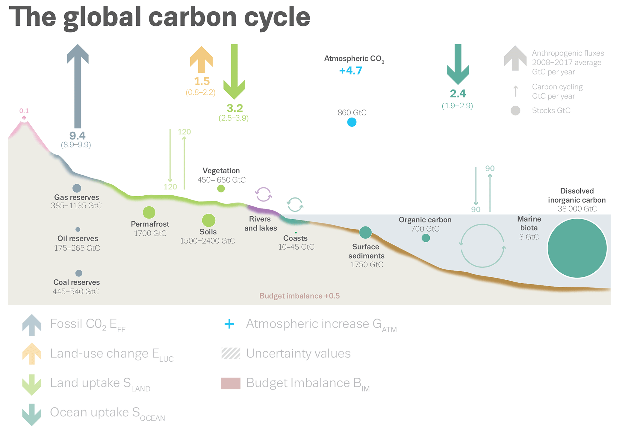
Figure 2Schematic representation of the overall perturbation of the global carbon cycle caused by anthropogenic activities, averaged globally for the decade 2008–2017. See legends for the corresponding arrows and units. The uncertainty in the atmospheric CO2 growth rate is very small (±0.02 GtC yr−1) and is neglected for the figure. The anthropogenic perturbation occurs on top of an active carbon cycle, with fluxes and stocks represented in the background and taken from Ciais et al. (2013) for all numbers, with the ocean fluxes updated to 90 GtC yr−1 to account for the increase in atmospheric CO2 since publication, and except for the carbon stocks at the coasts, which are from a literature review of coastal marine sediments (Price and Warren, 2016).
Other anthropogenic changes in the sources of CO and CH4 from wildfires, vegetation biomass, wetlands, ruminants, or permafrost changes are similarly assumed to have a small effect on the CO2 growth rate. The CH4 emissions and sinks are published and analysed separately in the Global Methane Budget publication that follows an approach similar to that presented here (Saunois et al., 2016).
2.8.2 Contribution of other carbonates to CO2 emissions
The contribution of fossil carbonates other than cement production is not systematically included in estimates of EFF, except at the national level at which they are accounted for in the UNFCCC national inventories. The missing processes include CO2 emissions associated with the calcination of lime and limestone outside cement production and the reabsorption of CO2 by the rocks and concrete from carbonation through their lifetime (Xi et al., 2016). Carbonates are used in various industries, including in iron and steel manufacture and in agriculture. They are found naturally in some coals. Carbonation from the cement life cycle, including demolition and crushing, was estimated by one study to be around 0.25 GtC yr−1 for the year 2013 (Xi et al., 2016). Carbonation emissions from the cement life cycle would offset calcination emissions from lime and limestone production. The balance of these two processes is not clear.
2.8.3 Anthropogenic carbon fluxes in the land-to-ocean aquatic continuum
The approach used to determine the global carbon budget refers to the mean, variations, and trends in the perturbation of CO2 in the atmosphere, referenced to the pre-industrial era. Carbon is continuously displaced from the land to the ocean through the land–ocean aquatic continuum (LOAC) comprising freshwaters, estuaries, and coastal areas (Bauer et al., 2013; Regnier et al., 2013). A significant fraction of this lateral carbon flux is entirely “natural” and is thus a steady-state component of the pre-industrial carbon cycle. We account for this pre-industrial flux where appropriate in our study. However, changes in environmental conditions and land use change have caused an increase in the lateral transport of carbon into the LOAC – a perturbation that is relevant for the global carbon budget presented here.
The results of the analysis of Regnier et al. (2013) can be summarised in two points of relevance for the anthropogenic CO2 budget. First, the anthropogenic perturbation has increased the organic carbon export from terrestrial ecosystems to the hydrosphere at a rate of 1.0±0.5 GtC yr−1, mainly owing to enhanced carbon export from soils. Second, this exported anthropogenic carbon is partly respired through the LOAC, partly sequestered in sediments along the LOAC, and to a lesser extent transferred to the open ocean where it may accumulate. The increase in storage of land-derived organic carbon in the LOAC and open ocean combined is estimated by Regnier et al. (2013) at 0.65±0.35 GtC yr−1. We do not attempt to incorporate the changes in LOAC in our study.
The inclusion of freshwater fluxes of anthropogenic CO2 affects the estimates of, and partitioning between, SLAND and SOCEAN in Eq. (1), but does not affect the other terms. This effect is not included in the GOBMs and DGVMs used in our global carbon budget analysis presented here.
2.8.4 Loss of additional sink capacity
Historical land-cover change was dominated by transitions from vegetation types that can provide a large sink per area unit (typically forests) to others less efficient in removing CO2 from the atmosphere (typically croplands). The resultant decrease in land sink, called the “loss of sink capacity”, is calculated as the difference between the actual land sink under changing land cover and the counterfactual land sink under pre-industrial land cover. An efficient protocol has yet to be designed to estimate the magnitude of the loss of additional sink capacity in DGVMs. Here, we provide a quantitative estimate of this term to be used in the discussion. Our estimate uses the compact Earth system model OSCAR whose land carbon cycle component is designed to emulate the behaviour of DGVMs (Gasser et al., 2017). We use OSCAR v2.2.1 (an update of v2.2 with minor changes) in a probabilistic setup identical to the one of Arneth et al. (2017) but with a Monte Carlo ensemble of 2000 simulations. For each, we calculate SLAND and the loss of additional sink capacity separately. We then constrain the ensemble by weighting each member to obtain a distribution of cumulative SLAND over 1850–2005 close to the DGVMs used here. From this ensemble, we estimate a loss of additional sink capacity of 0.4±0.3 GtC yr−1 on average over 2005–2014 and 20±15 GtC accumulated between 1870 and 2017 (using a linear extrapolation of the trend to estimate the last few years).
3.1 Global carbon budget mean and variability for 1959–2017
The global carbon budget averaged over the last half-century is shown in Fig. 3. For this time period, 82 % of the total emissions (EFF+ELUC) were caused by fossil CO2 emissions and 18 % by land-use change. The total emissions were partitioned among the atmosphere (45 %), ocean (24 %), and land (30 %). All components except land-use change emissions have grown since 1959, with important interannual variability in the growth rate in atmospheric CO2 concentration and in the land CO2 sink (Fig. 4) and some decadal variability in all terms (Table 6). Differences with previous budget releases are documented in Fig. B4.

Figure 3Combined components of the global carbon budget illustrated in Fig. 2 as a function of time, for fossil CO2 emissions (EFF; grey) and emissions from land-use change (ELUC; brown), as well as their partitioning among the atmosphere (GATM; blue), ocean (SOCEAN; turquoise), and land (SLAND; green). The partitioning is based on nearly independent estimates from observations (for GATM) and from process model ensembles constrained by data (for SOCEAN and SLAND) and does not exactly add up to the sum of the emissions, resulting in a budget imbalance, which is represented by the difference between the bottom pink line (reflecting total emissions) and the sum of the ocean, land, and atmosphere. All time series are in GtC yr−1. GATM and SOCEAN prior to 1959 are based on different methods. EFF values are primarily from Boden et al. (2017), with uncertainty of about ±5 % (±1σ); ELUC values are from two bookkeeping models (Table 2) with uncertainties of about ±50 %; GATM prior to 1959 is from Joos and Spahni (2008) with uncertainties equivalent to about ±0.1–0.15 GtC yr−1 and from Dlugokencky and Tans (2018) from 1959 with uncertainties of about ±0.2 GtC yr−1; SOCEAN prior to 1959 is averaged from Khatiwala et al. (2013) and DeVries (2014) with uncertainty of about ±30 % and from a multi-model mean (Table 4) from 1959 with uncertainties of about ±0.5 GtC yr−1; SLAND is a multi-model mean (Table 4) with uncertainties of about ±0.9 GtC yr−1. See the text for more details of each component and their uncertainties.
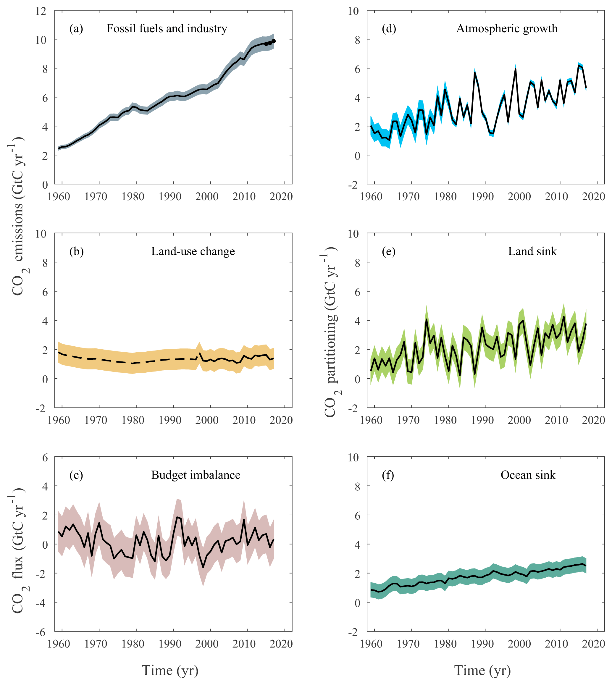
Figure 4Components of the global carbon budget and their uncertainties as a function of time, presented individually for (a) fossil CO2 emissions (EFF), (b) emissions from land-use change (ELUC), (c) the budget imbalance that is not accounted for by the other terms, (d) growth rate in atmospheric CO2 concentration (GATM), (e) the land CO2 sink (SLAND, positive indicates a flux from the atmosphere to the land), and (f) the ocean CO2 sink (SOCEAN, positive indicates a flux from the atmosphere to the ocean). All time series are in GtC yr−1 with the uncertainty bounds representing ±1σ in shaded colours. Data sources are as in Fig. 3. The black dots in (a) show values for 2015–2017 that originate from a different data set to the remainder of the data (see text). The dashed line in (b) identifies the pre-satellite period before the inclusion of peatland burning.
Table 6Decadal mean in the five components of the anthropogenic CO2 budget for different periods and the last year available. All values are in GtC yr−1, and uncertainties are reported as ±1σ. The table also shows the budget imbalance (BIM), which provides a measure of the discrepancies among the nearly independent estimates and has an uncertainty exceeding ±1 GtC yr−1. A positive imbalance means the emissions are overestimated and/or the sinks are too small.
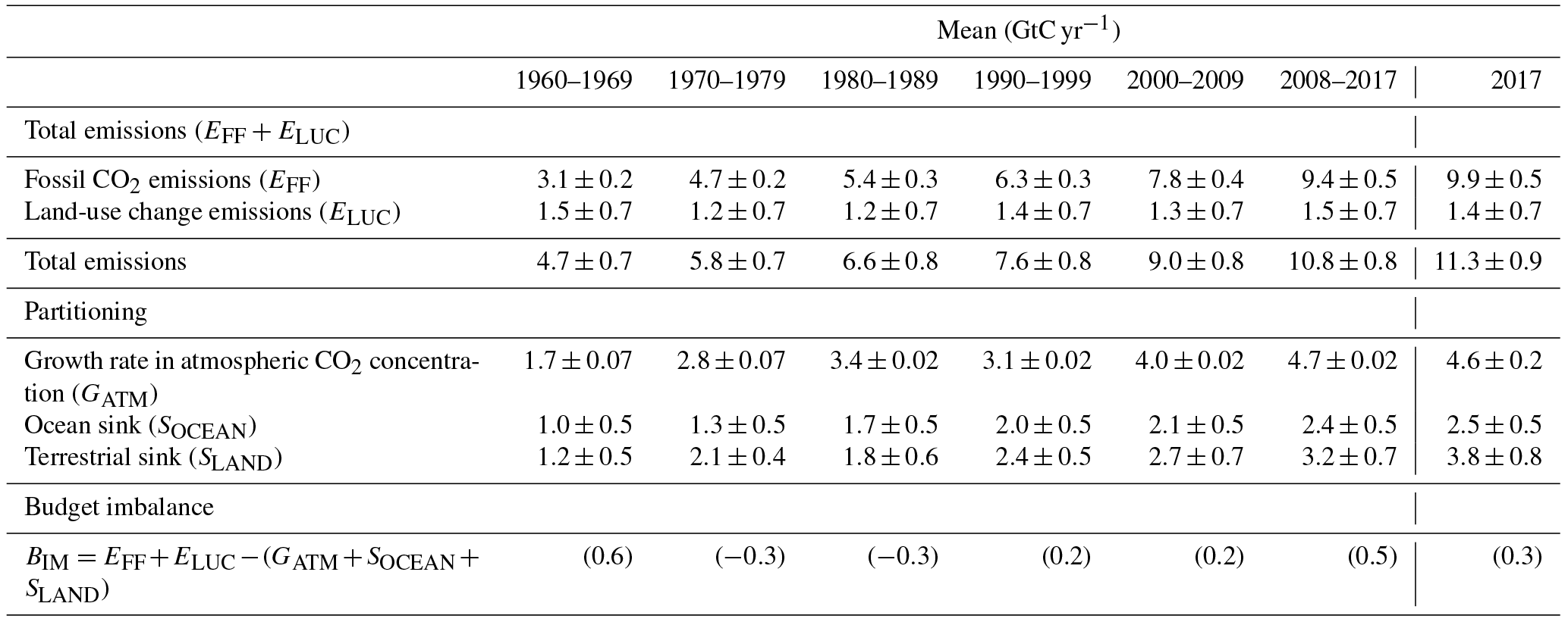
3.1.1 CO2 emissions
Global fossil CO2 emissions have increased every decade from an average of 3.1±0.2 GtC yr−1 in the 1960s to an average of 9.4±0.5 GtC yr−1 during 2008–2017 (Table 6, Figs. 2 and 5). The growth rate in these emissions decreased between the 1960s and the 1990s, from 4.5 % yr−1 in the 1960s (1960–1969) to 2.8 % yr−1 in the 1970s (1970–1979), 1.9 % yr−1 in the 1980s (1980–1989), and 1.0 % yr−1 in the 1990s (1990–1999). After this period, the growth rate began increasing again in the 2000s at an average growth rate of 3.2 % yr−1, decreasing to 1.5 % yr−1 for the last decade (2008–2017), with a 3-year period of no or low growth during 2014–2016 (Fig. 5).

Figure 5Fossil CO2 emissions for (a) the globe, including an uncertainty of ±5 % (grey shading), and the emissions extrapolated using BP energy statistics (black dots); (b) global emissions by fuel type, including coal (salmon), oil (olive), gas (turquoise), and cement (purple), and excluding gas flaring, which is small (0.6 % in 2013); (c) territorial (solid lines) and consumption (dashed lines) emissions for the top three country emitters (US – olive; China – salmon; India – purple) and for the European Union (EU; turquoise for the 28 member states of the EU as of 2012); and (d) per capita emissions for the top three country emitters, the EU (all colours as in panel c), and the world (black). In (b–c), the dots show the data that were extrapolated from BP energy statistics for 2014–2016. All time series are in GtC yr−1 except the per capita emissions (d), which are in tonnes of carbon per person per year (tC person−1 yr−1). Territorial emissions are primarily from Boden et al. (2017) except national data for the US and EU28 (the 28 member states of the EU) for 1990–2016, which are reported by the countries to the UNFCCC as detailed in the text; consumption-based emissions are updated from Peters et al. (2011a). See Sect. 2.1.1 for details of the calculations and data sources.
In contrast, CO2 emissions from land use, land-use change, and forestry have remained relatively constant, at around 1.3±0.7 GtC yr−1 over the past half-century but with large spread across estimates (Fig. 6). These emissions are also relatively constant in the DGVM ensemble of models, except during the last decade when they increase to 1.9±0.6 GtC yr−1. However, there is no agreement on this recent increase between the two bookkeeping models, each suggesting an opposite trend (Fig. 6).
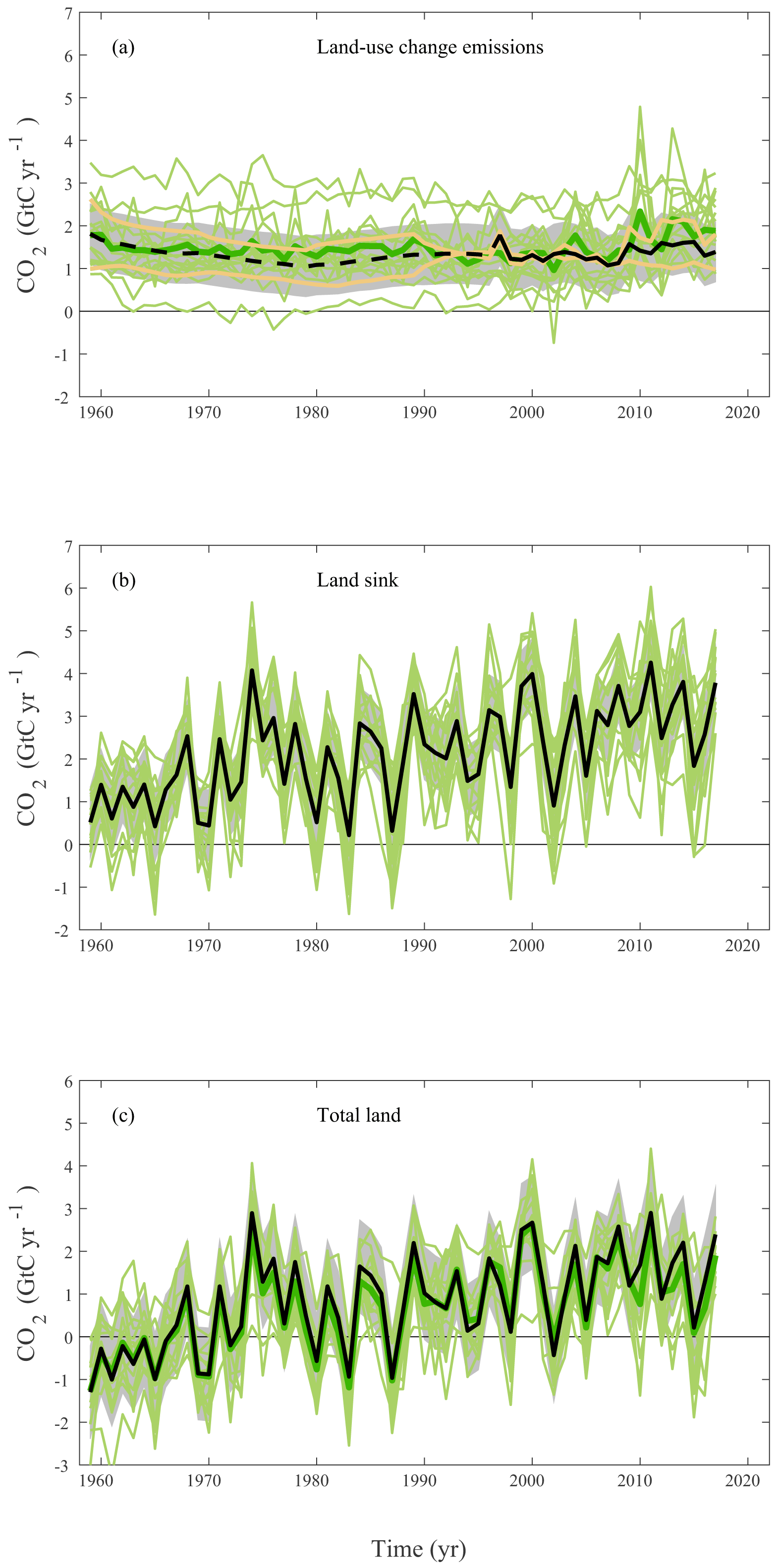
Figure 6CO2 exchanges between the atmosphere and the terrestrial biosphere as used in the global carbon budget (black with ±1σ uncertainty in grey shading), for (a) CO2 emissions from land-use change (ELUC), also individually showing the two bookkeeping models (two brown lines) and the DGVM model results (green) and their multi-model mean (dark green). The dashed line identifies the pre-satellite period before the inclusion of peatland burning. (b) Land CO2 sink (SLAND) with individual DGVMs (green); (c) total land CO2 fluxes (b–a) with individual DGVMs (green) and their multi-model mean (dark green).
3.1.2 Partitioning among the atmosphere, ocean, and land
The growth rate in atmospheric CO2 level increased from 1.7±0.07 GtC yr−1 in the 1960s to 4.7±0.02 GtC yr−1 during 2008–2017 with important decadal variations (Table 6 and Fig. 2). Both ocean and land CO2 sinks increased roughly in line with the atmospheric increase, but with significant decadal variability on land (Table 6), and possibly in the ocean (Fig. 7).
The ocean CO2 sink increased from 1.0±0.5 GtC yr−1 in the 1960s to 2.4±0.5 GtC yr−1 during 2008–2017, with interannual variations of the order of a few tenths of GtC yr−1 generally showing an increased ocean sink during large El Niño events (i.e. 1997–1998) (Fig. 7; Rödenbeck et al., 2014). Although there is some coherence among the GOBMs and pCO2-based flux products regarding the mean, there is poor agreement for interannual variability, and the ocean models underestimate decadal variability (Sect. 2.5.3 and Fig. 7; DeVries et al., 2017).

Figure 7Comparison of the anthropogenic atmosphere–ocean CO2 flux showing the budget values of SOCEAN (black; with ±1σ uncertainty in grey shading), individual ocean models (blue), and the two ocean pCO2-based flux products (dark blue; see Table 4). Both pCO2-based flux products were adjusted for the pre-industrial ocean source of CO2 from river input to the ocean, which is not present in the ocean models, by adding a sink of 0.78 GtC yr−1 (Resplandy et al., 2018), to make them comparable to SOCEAN. This adjustment does not take into account the anthropogenic contribution to river fluxes (see Sect. 2.8.3).
The terrestrial CO2 sink increased from 1.2±0.5 GtC yr−1 in the 1960s to 3.2±0.7 GtC yr−1 during 2008–2017, with important interannual variations of up to 2 GtC yr−1 generally showing a decreased land sink during El Niño events (Fig. 6), responsible for the corresponding enhanced growth rate in atmospheric CO2 concentration. The larger land CO2 sink during 2008–2017 compared to the 1960s is reproduced by all the DGVMs in response to the combined atmospheric CO2 increase and changes in climate, and consistent with constraints from the other budget terms (Table 5).
Estimates of total atmosphere-to-land fluxes (SLAND–ELUC) from the DGVMs are consistent with the budget constraints (Table 5), except during 2008–2017, when the DGVM ensemble estimates a total atmosphere-to-land flux of 1.3±0.5 GtC yr−1, likely below the budget constraints of 2.1±0.7 GtC yr−1 and outside the range of the inversions (Table 5). This comparison suggests that the DGVMs could overestimate ELUC emissions and/or underestimate the terrestrial sink SLAND during the last decade.
3.1.3 Model evaluation
The evaluation of ocean estimates (Fig. B1) shows a relative interannual mismatch of 15 % and 17 % for the two pCO2-based flux products over the globe, relative to the pCO2 observations from the SOCAT v6 database for the period 1985–2017. A 0 % mismatch would indicate a perfect model, and a field with no interannual variability would result in a 100 % mismatch. A mismatch larger than 100 % is possible when the method produces a larger mismatch than the benchmark field with no interannual variability (see Sect. 2.5.3). This mismatch by the pCO2-based flux products is improved compared with earlier published versions of these two flux products of around 20 %–25 % for the 1992–2009 time period (Rödenbeck et al., 2015), likely because of the larger data availability after 2009. The GOBMs show a global relative interannual mismatch between 50 % and 60 %, with one model at 94 % and one at 193 %. The GOBM mismatch is of the same order as the mismatch calculated in an ensemble of 14 flux products but larger than the two flux products used in this report (Fig. 5 in Rödenbeck et al., 2015). The mismatch is generally larger at high latitudes compared to the tropics, for both the flux products and the GOBMs. The two flux products have a similar mismatch of around 10 %–15 % in the tropics, around 25 % in the north, and 30 %–55 % in the south. The GOBM mismatch is more spread across regions, ranging from 29 % to 178 % in the tropics, 70 % to 192 % in the north, and 108 % to 304 % in the south. The higher mismatch occurs in regions with stronger climate variability, such as the northern and southern high latitudes (poleward of the subtropical gyres) and the equatorial Pacific. The latter is also apparent in the model mismatch but is hidden in Fig. B1 due to the averaging over 30∘ S to 30∘ N (see also Sect. 4).
The evaluation of the DGVMs (Fig. B2) shows generally high skill scores across models for runoff, and to a lesser extent for vegetation biomass, GPP, and ecosystem respiration (Fig. B2, left panel). The skill score was lowest for leaf area index and net ecosystem exchange, with the widest disparity among models for soil carbon. Further analysis of the results will be provided separately, focusing on the strengths and weaknesses in the DGVM ensemble and its validity for use in the global carbon budget.
The evaluation of the atmospheric inversions (Fig. B3) shows long-term mean biases in the free troposphere better than 0.8 ppm in absolute values for each product. CAMS and CTE biases show some dependency on latitude (a trend of and 0.0043±0.0004 ppm per degree for CAMS and CTE, respectively). These latitude-dependent biases may reveal biases in the surface fluxes (e.g. Houweling et al., 2015) but the link is not straightforward and will be analysed separately. The biases for MIROC and CarboScope behave similarly together in relative values, but they are less regular than the two other products, which hampers the interpretation. Lesser model performance for specific aircraft programmes, like for the 4-year DISCOVER-AQ campaign in the continental US (https://discover-aq.larc.nasa.gov/, last access: 28 November 2018), contributes to this variability.
3.1.4 Budget imbalance
The carbon budget imbalance (BIM; Eq. 1) quantifies the mismatch between the estimated total emissions and the estimated changes in the atmosphere, land, and ocean reservoirs. The mean budget imbalance from 1959 to 2017 is small (0.14 GtC yr−1) and shows no trend over the full time series. The process models (GOBMs and DGVMs) have been selected to match observational constraints in the 1990s but no further constraints have been applied to their representation of trend and variability. Therefore, the near-zero mean and trend in the budget imbalance are indirect evidence of a coherent community understanding of the emissions and their partitioning on those timescales (Fig. 4). However, the budget imbalance shows substantial variability on the order of ±1 GtC yr−1, particularly over semi-decadal timescales, although most of the variability is within the uncertainty of the estimates. The positive carbon imbalance during the 1960s, early 1990s, and in the last decade suggests that either the emissions were overestimated or the sinks were underestimated during these periods. The reverse is true for the 1970s and around 1995–2000 (Fig. 4).
We cannot attribute the cause of the variability in the budget imbalance with our analysis, only to note that the budget imbalance is unlikely to be explained by errors or biases in the emissions alone because of its large semi-decadal variability component, a variability that is untypical of emissions and has not changed in the past 50 years in spite of a nearly tripling in emissions (Fig. 4). Errors in SLAND and SOCEAN are more likely to be the main cause for the budget imbalance. For example, underestimation of SLAND by DGVMs has been reported following the eruption of Mount Pinatubo in 1991 possibly due to missing responses to changes in diffuse radiation (Mercado et al., 2009) or other yet unknown factors, and DGVMs are suspected to overestimate the land sink in response to the wet decade of the 1970s (Sitch et al., 2008). Decadal and semi-decadal variability in the ocean sink has been also reported recently (DeVries et al., 2017; Landschützer et al., 2015), with the pCO2-based ocean flux products suggesting a smaller-than-expected ocean CO2 sink in the 1990s and a larger-than-expected sink in the 2000s (Fig. 7), possibly caused by changes in ocean circulation (DeVries et al., 2017) not captured in coarse-resolution GOBMs used here (Dufour et al., 2013). The absence of internal variability could also be at fault. Internal variability is not captured by single realisations of coarse-resolution model simulations (Li and Ilyina, 2018) and is thought to be largest in regions with strong seasonal and interannual climate variability, i.e. the high-latitude ocean regions (poleward of the subtropical gyres) and the equatorial Pacific (McKinley et al., 2016). Some of these errors could be driven by errors in the climatic forcing data, particularly precipitation (for SLAND) and wind (for SOCEAN), rather than in the models.
3.2 Global carbon budget for the last decade (2008–2017)
The global carbon budget averaged over the last decade (2008–2017) is shown in Figs. 2 and 9. For this time period, 87 % of the total emissions (EFF+ELUC) were from fossil CO2 emissions (EFF) and 13 % were from land-use change (ELUC). The total emissions were partitioned among the atmosphere (44 %), ocean (22 %), and land (29 %), with a remaining unattributed budget imbalance (5 %).
3.2.1 CO2 emissions
Global fossil CO2 emissions grew at a rate of 1.5 % yr−1 for the last decade (2008–2017). China's emissions increased by +3.0 % yr−1 on average (increasing by +0.64 GtC yr−1 during the 10-year period), dominating the global trends, followed by India's emissions increase by +5.2 % yr−1 (increasing by +0.25 GtC yr−1), while emissions decreased in the EU28 by −1.8 % yr−1 (decreasing by −0.17 GtC yr−1), and in the US by 0.9 % yr−1 (decreasing by −0.18 GtC yr−1). In the past decade, fossil CO2 emissions decreased significantly (at the 95 % level) in 25 countries: Aruba, Barbados, Croatia, Czech Republic, North Korea, Denmark, France, Greece, Greenland, Iceland, Ireland, Malta, the Netherlands, Romania, Slovakia, Slovenia, Sweden, Switzerland, Syria, Trinidad and Tobago, Ukraine, the United Kingdom, the US, Uzbekistan, and Venezuela. Notable was Germany, whose emissions did not decrease significantly.
In contrast, there is no apparent trend in CO2 emissions from land-use change (Fig. 6), though the data are very uncertain, with the two bookkeeping estimates showing opposite trends over the last decade. Larger emissions are expected increasingly over time for DGVM-based estimates as they include the loss of additional sink capacity, while the bookkeeping estimates do not. The LUH2 data set also features large dynamics in land use in particular in the tropics in recent years, causing higher emissions in DGVMs and BLUE than in H&N.
3.2.2 Partitioning among the atmosphere, ocean, and land
The growth rate in atmospheric CO2 concentration increased during 2008–2017, in contrast to more constant levels the previous decade and reflecting a similar decrease in the land sink compared to an increase in the previous decade, albeit with large interannual variability (Fig. 4). During the same period, the ocean CO2 sink appears to have intensified, an effect which is particularly apparent in the pCO2-based flux products (Fig. 7) and is thought to originate at least in part in the Southern Ocean (Landschützer et al., 2015).
The budget imbalance (Table 6) and the residual sink from the global budget (Table 5) include an error term due to the inconsistency that arises from using ELUC from bookkeeping models but SLAND from DGVMs. This error term includes the fundamental differences between bookkeeping models and DGVMs, most notably the loss of additional sink capacity. Other differences include an incomplete account of land-use change practices and processes in DGVMs, while they are all accounted for in bookkeeping models by using observed carbon densities, and bookkeeping error of keeping present-day carbon densities fixed in the past. That the budget imbalance shows no clear trend towards larger values over time is an indication that the loss of additional sink capacity plays a minor role compared to other errors in SLAND or SOCEAN (discussed in Sect. 3.1.4).
3.2.3 Regional distribution
Figure 8 shows the partitioning of the total atmosphere-to-surface fluxes excluding fossil CO2 emissions () according to the multi-model average of the process models in the ocean and on land (GOBMs and DGVMs) and to the atmospheric inversions. Figure 8 provides information on the regional distribution of those fluxes by latitude bands. The global mean total atmosphere-to-surface CO2 fluxes from process models for 2008–2017 is 3.7±1.2 GtC yr−1. This is below but still within the uncertainty range of a global mean atmosphere-to-surface flux of 4.6±0.5 GtC yr−1 inferred from the carbon budget (EFF–GATM in Eq. 1; Table 6). The total atmosphere-to-surface CO2 fluxes from the four inversions are very similar, ranging from 4.7 to 5.0 GtC yr−1, consistent with the carbon budget as expected from the constraints on the inversions and the adjustments to the same EFF distribution (see Sect. 2.7).
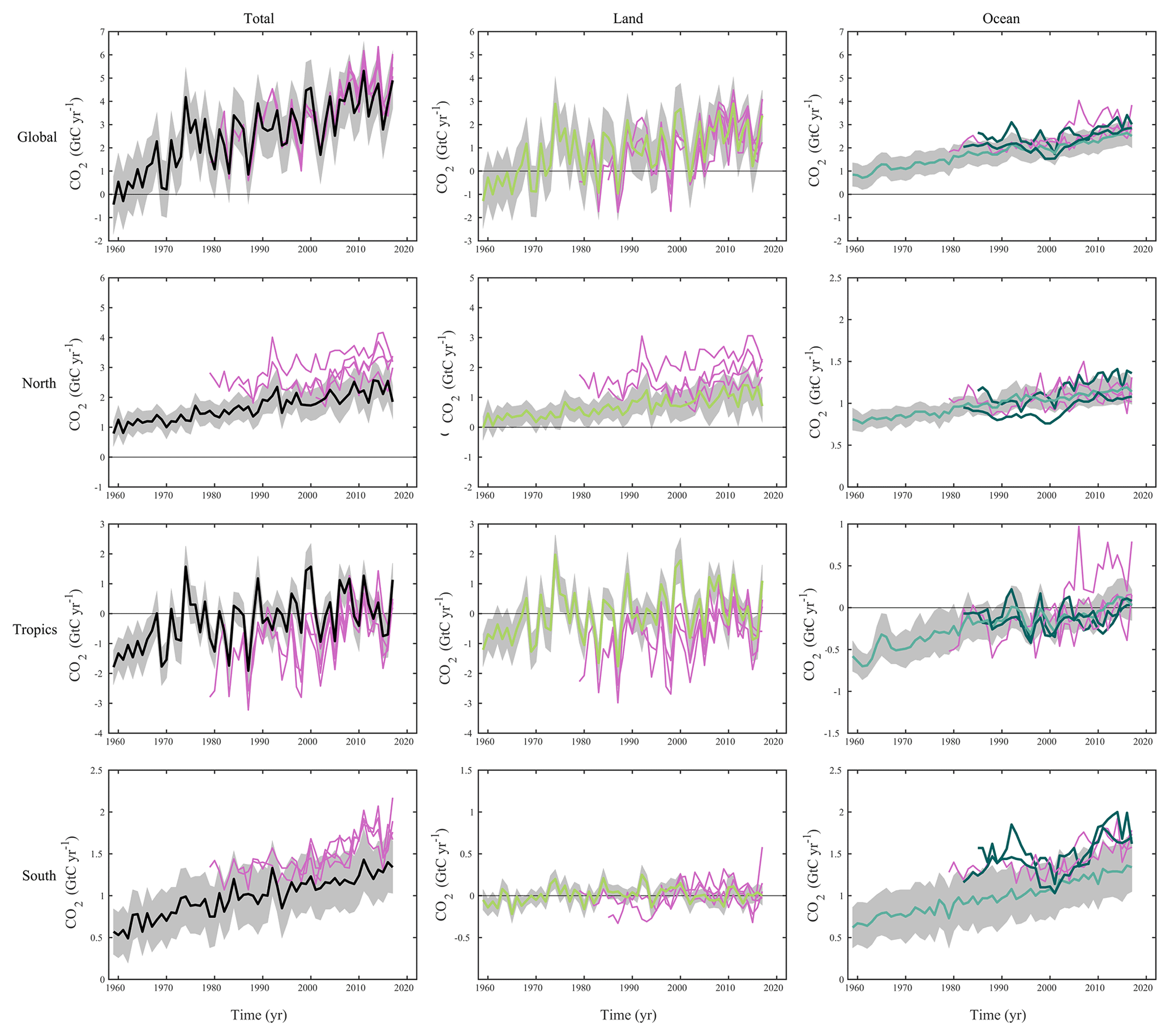
Figure 8CO2 fluxes between the atmosphere and the surface () by latitude bands for the (top) globe (second row), north (north of 30∘ N), (third row) tropics (30∘ S–30∘ N), and (bottom) south (south of 30∘ S) and (left) total, (middle) land only (SLAND−ELUC), and (right) ocean only. Positive values indicate a flux from the atmosphere to the land and/or ocean. Estimates from the combination of the process models for the land and oceans are shown (black for the total, green for the land, blue for the ocean) with ±1σ of the model ensemble (in grey). Results from the atmospheric inversions (pink lines) and from the pCO2-based flux products (dark blue lines) are also shown.
In the south (south of 30∘ S), the atmospheric inversions suggest an atmosphere-to-surface flux for 2008–2017 of around 1.6–1.7 GtC yr−1, close to the process models' estimate of 1.4±0.7 GtC yr−1 (Fig. 8). The interannual variability in the south is low because of the dominance of ocean area with low variability compared to land areas. The split between land (SLAND−ELUC) and ocean (SOCEAN) shows a small contribution to variability in the south coming from the land, with no consistency between the DGVMs and the inversions or among inversions. This is expected due to the difficulty of separating exactly the land and oceanic fluxes when viewed from atmospheric observations alone. The oceanic variability in the south is estimated to be significant in the two flux products and in at least one of the inversions, with decadal variability in around 0.5 GtC yr−1. The GOBMs do not reproduce this variability.
In the tropics (30∘ S–30∘ N), both the atmospheric inversions and process models suggest the total carbon balance in this region is close to neutral on average over the past decade, with atmosphere-to-surface fluxes for the 2008–2017 average ranging between −0.4 and +0.4 GtC yr−1. The agreement between inversions and models is significantly better for the last decade than for any previous decade, although the reasons for this better agreement are still unclear. Both the process models and the inversions consistently allocate more year-to-year variability in CO2 fluxes to the tropics compared to the north (north of 30∘ N; Fig. 8). The split between the land and ocean indicates the land is the origin of most of the tropical variability, consistently among models (both for the land and for the ocean) and inversions. The oceanic variability in the tropics is similar among models and with the two ocean flux products, reflected in their lower observational mismatch (Sect. 3.1.3). While the inversions indicate that atmosphere-to-land CO2 fluxes are more variable than atmosphere-to-ocean CO2 fluxes in the tropics, the correspondence between the inversions and the ocean flux products or GOBMs is much poorer.
In the north (north of 30∘ N), the inversions and process models show less agreement on the magnitude of the atmosphere-to-land flux, with the ensemble mean of the process models suggesting a total Northern Hemisphere sink for 2008–2017 of 2.2±0.6 GtC yr−1, likely below the estimates from the inversions ranging from 2.6 to 3.6 GtC yr−1 (Fig. 8). The discrepancy in the north-tropics distribution of CO2 fluxes between the inversions and models arises from the differences in mean fluxes over the northern land. This discrepancy is also evidenced over the previous decade and highlights not only persistent issues with the quantification of the drivers of the net land CO2 flux (Arneth et al., 2017; Huntzinger et al., 2017) but also the distribution of atmosphere-to-land fluxes between the tropics and higher latitudes that is particularly marked in previous decades, as highlighted previously (Stephens et al., 2007; Baccini et al., 2017; Schimel et al., 2015).
Differences between inversions may be related for example to differences in their interhemispheric transport, and other inversion settings (Table A3). Separate analysis has shown that the influence of the chosen prior land and ocean fluxes is minor compared to other aspects of each inversion. In comparison to the previous global carbon budget publication, the fossil fuel inputs were adjusted to match those of EFF used in this analysis (see Sect. 2.7), therefore removing differences due to prior fossil emissions. Differences between inversions and the ensemble of process models in the north cannot be simply explained. They could either reflect a bias in the inversions or missing processes or biases in the process models, such as the lack of adequate parameterisations for forest management in the north and for forest degradation emissions in the tropics for the DGVMs. The estimated contribution of the north and its uncertainty from process models is sensitive to both the ensemble of process models used and the specifics of each inversion.
Resolving the differences in the Northern Hemisphere land sink will require the consideration and inclusion of larger volumes of semi-continuous observations from tall towers close to the surface CO2 exchange. Some of these data are becoming available but not used in the current inverse models, sometimes due to the short records and sometimes because the coarse transport models cannot adequately represent these time series. Improvements in model resolution and atmospheric transport realism together with expansion of the observational record (also in the data-sparse Boreal Eurasian area) will help anchor the mid-latitude fluxes per continent. In addition, new metrics could potentially differentiate between the more and less realistic realisations of the Northern Hemisphere land sink shown in Fig. 8.
3.2.4 Budget imbalance
The budget imbalance was +0.5 GtC yr−1 on average over 2008–2017. Although the uncertainties are large in each term, the sustained imbalance over this last decade suggests an overestimation of the emissions and/or an underestimation of the sinks. An origin in the land and/or ocean sink may be more likely, given the large variability in the land sink and the suspected underestimation of decadal variability in the ocean sink. An underestimate of SLAND would also reconcile model results with inversion estimates for fluxes in the total land during the past decade (Fig. 8; Table 5). However, we cannot exclude that the budget imbalance over the last decade could partly be due to an overestimation of CO2 emissions from land-use change, given their large uncertainty, as has been suggested elsewhere (Piao et al., 2018). More integrated use of observations in the Global Carbon Budget, either on their own or for further constraining model results, should help resolve some of the budget imbalance (Peters et al., 2017; Sect. 4).
3.3 Global carbon budget for the year 2017
3.3.1 CO2 emissions
Preliminary estimates of global fossil CO2 emissions based on BP energy statistics are for emissions growing by 1.6 % between 2016 and 2017 to 9.9±0.5 GtC in 2017 (Fig. 5), distributed among coal (40 %), oil (35 %), gas (20 %), cement (4 %), and gas flaring (0.7 %). Compared to the previous year, emissions from coal increased by 1.6 %, while emissions from oil, gas, and cement increased by 1.7 %, 3.0 %, and 1.2 %, respectively. All growth rates presented are adjusted for the leap year, unless stated otherwise.
The growth in emissions of 1.6 % in 2017 is within the range of the projected growth of 2.0 % (range of 0.8 to 3.0 %) published in Le Quéré et al. (2018) based on national emission projections for China, the US, and India and projections of gross domestic product corrected for IFF trends for the rest of the world. The growth in emissions in 2017 for China, the US, and the rest of the world is also within their previously projected range, while the growth in India was slightly above the projection (Table 7).
Table 7Comparison of the projection with realised fossil CO2 emissions (EFF). The “Actual” values are the first estimate available using actual data, and the “Projected” values refer to the estimate made before the end of the year for each publication. Projections based on a different method from that described here during 2008–2014 are available in Le Quéré et al. (2016). All values are adjusted for leap years.
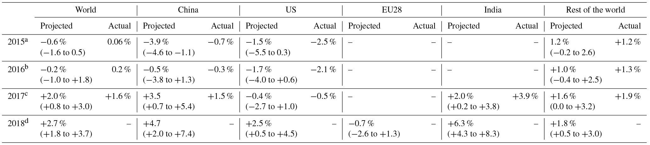
a Jackson et al. (2016) and Le Quéré et al. (2015a). b Le Quéré et al. (2016). c Le Quéré et al. (2018). d This study.
In 2017, the largest absolute contributions to global CO2 emissions were from China (27 %), the US (15 %), the EU (28 member states; 10 %), and India (7 %) while the rest of the world contributed 42 %. The percentages are the fraction of the global emissions including bunker fuels (3.1 %). These four regions account for 59 % of global CO2 emissions. Growth rates for these countries from 2016 to 2017 were +1.5 % (China), −0.5 % (US), +1.2 % (EU28), and +3.9 % (India), with +1.9 % for the rest of the world. The per capita CO2 emissions in 2017 were 1.1 tC person−1 yr−1 for the globe and were 4.4 (US), 2.0 (China), 1.9 (EU28), and 0.5 (India) tC person−1 yr−1 for the four highest emitting countries (Fig. 5).
In 2016 (the last year available), the largest absolute contributions to global CO2 emissions from a consumption perspective were China (25 %), the US (16 %), the EU (12 %), and India (6 %). The difference between territorial and consumption emissions (the net emission transfer via international trade) has generally increased from 1990 to around 2005 and remained relatively stable afterwards until the last year available (2016; Fig. 5).
The global CO2 emissions from land-use change are estimated as 1.4±0.7 GtC in 2017, close to the previous decade but with low confidence in the annual change. This brings the total CO2 emissions from fossil fuels plus land-use change (EFF+ELUC) to 11.3±0.9 GtC (41.2±3 GtCO2).
3.3.2 Partitioning among the atmosphere, ocean, and land
The growth rate in atmospheric CO2 concentration was 4.6±0.2 GtC in 2017 (2.16±0.09 ppm; Fig. 4; Dlugokencky and Tans, 2018). This is near the 2008–2017 average of 4.7±0.1 GtC yr−1 and reflects the return to normal conditions after the El Niño of 2015–2016.
The estimated ocean CO2 sink was 2.5±0.5 GtC in 2017. All models and data products estimate a small reduction or no change in the sink (average of 0.1, ranging from +0.02 to −0.4 GtC), consistent with the return to normal conditions after the El Niño, which caused an enhanced sink in previous years (Fig. 7).
The terrestrial CO2 sink from the model ensemble was 3.8±0.8 GtC in 2017, above the decadal average (Fig. 4) and consistent with constraints from the rest of the budget (Table 5).
The budget imbalance was +0.3 GtC in 2017, indicating, as for the last decade, a small overestimation of the emissions and/or underestimation of the sinks for that year. This imbalance is indicative only, given the large uncertainties in the estimation of the BIM.
3.4 Global carbon budget projection for the year 2018
3.4.1 CO2 emissions
Based on available data as of 7 November 2018 (see Sect. 2.1.5), fossil CO2 emissions (EFF) for 2018 are projected to increase by +2.7 % (range of 1.8 % to +3.7 %; Table 7). Our method contains several assumptions that could influence the estimate beyond the given range, and as such, it has an indicative value only. Within the given assumptions, global emissions would be 10.1±0.5 GtC (37.1±1.8 GtCO2) in 2018. The interpretation of the 2018 emission projection is provided elsewhere (Figueres et al., 2018; Jackson et al., 2018).
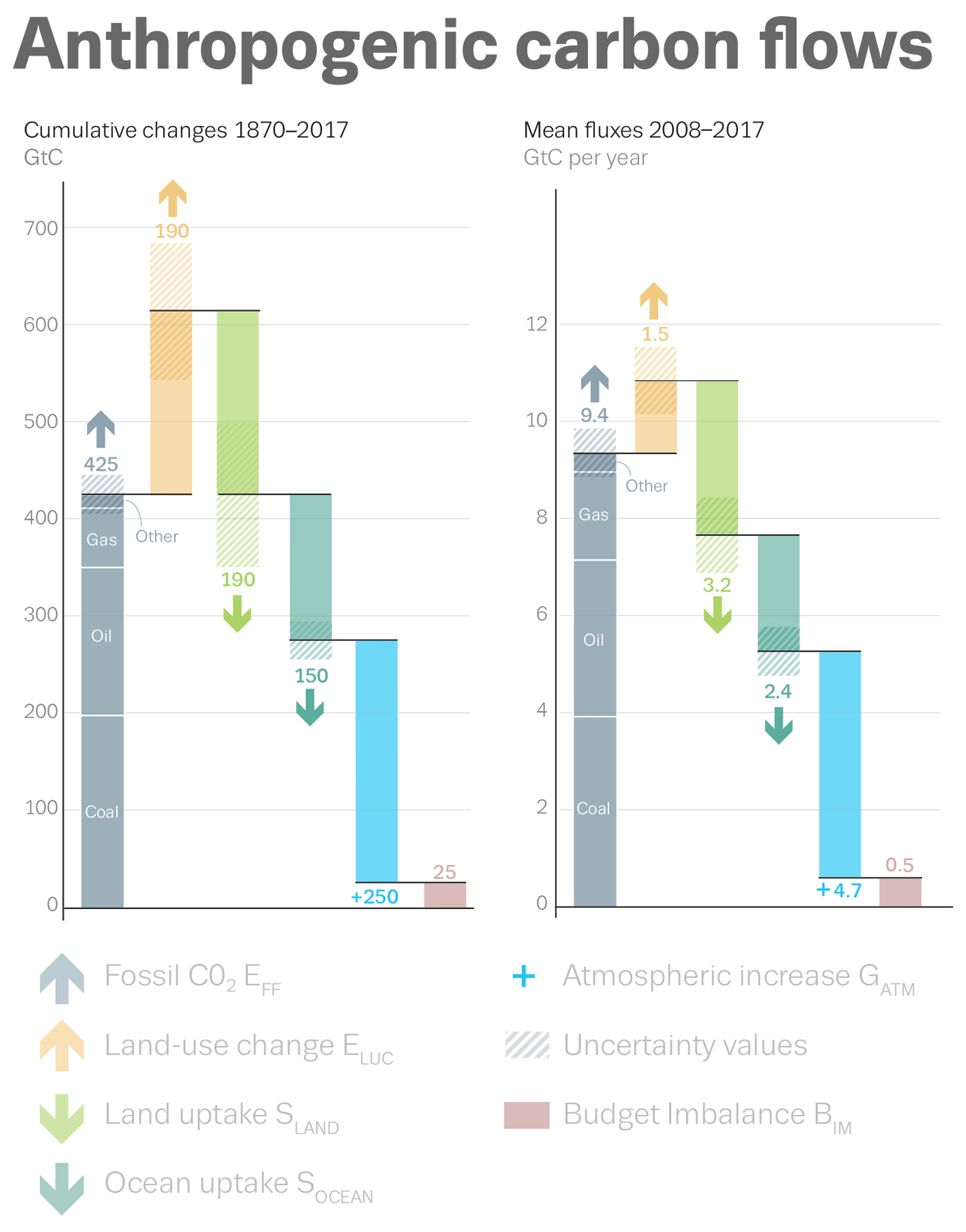
Figure 9Cumulative changes during 1870–2017 and mean fluxes during 2008–2017 for the anthropogenic perturbation as defined in the legend.
For China, the expected change is for an increase in emissions of +4.7 % (range of +2.0 % to +7.4 %) in 2018 compared to 2017. This is based on estimated growth in coal (+4.5 %; the main fuel source in China), oil (+3.6 %), natural gas (+17.7 %) consumption, and cement production (+1.0 %). The uncertainty range considers the variations in the difference between preliminary January–September data and final full-year data, the uncertainty in the preliminary data used for the 2017 base, and uncertainty in the evolution of energy density and carbon content of coal. See also Liu et al. (2018) for further analysis of China's projected emissions.
Table 8Cumulative CO2 for different time periods in gigatonnes of carbon (GtC). All uncertainties are reported as ±1σ. The budget imbalance provides a measure of the discrepancies among the nearly independent estimates. Its uncertainty exceeds ±60 GtC. The method used here does not capture the loss of additional sink capacity from reduced forest cover, which is about 20 GtC and would exacerbate the budget imbalance (see Sect. 2.8.4). All values are rounded to the nearest 5 GtC and therefore columns do not necessarily add to zero.
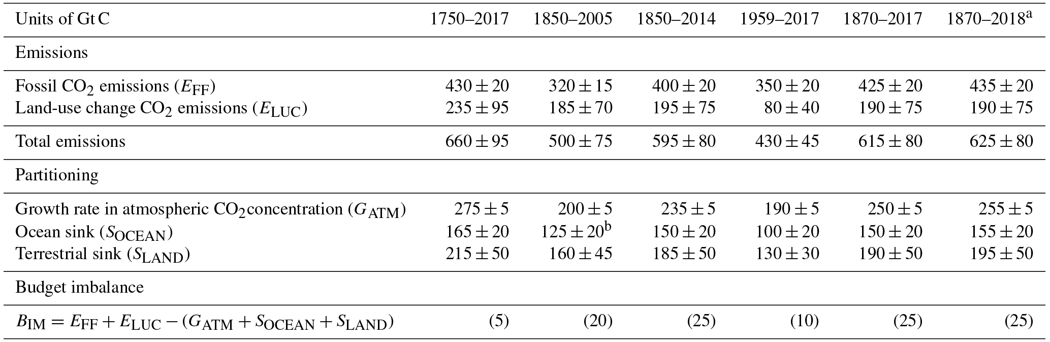
a Using projections for the year 2018 (Sect. 3.3). b This value was incorrectly reported as 145 in Le Quéré et al. (2018).
For the US, the EIA emission projection for 2018 combined with cement data from USGS give an increase of 2.5 % (range of +0.5 to +4.5 %) compared to 2017.
For the European Union, our projection for 2018 is for a decrease of −0.7 % (range of −2.6 % to +1.3 %) over 2017. This is based on estimates for coal of −1.2 %, oil of +1.2 %, gas of −2.9 %, and stable cement emissions.
For India, our projection for 2018 is for an increase of +6.3 % (range of 4.3 % to +8.3 %) over 2017. This is based on separate projections for coal (+7.1 %), oil (+2.9 %), gas (+6.0 %), and cement (+13.4 %).
For the rest of the world, the expected growth for 2018 is +1.8 % (range of +0.5 % to +3.0 %). This is computed using the GDP projection for the world excluding China, the US, the EU, and India of 2.8 % made by the IMF (IMF, 2018) and a decrease in IFF of −1.0 % yr−1, which is the average from 2008 to 2017. The uncertainty range is based on the standard deviation of the interannual variability in IFF during 2008–2017 of ±0.7 % yr−1 and our estimate of uncertainty in the IMF's GDP forecast of ±0.5 %.
Preliminary estimates of fire emissions in deforestation zones indicate that emissions from land-use change (ELUC) for 2018 were below average until October and are expected to range between 0.1 and 0.2 lower than the 2008–2017 average. We therefore expect ELUC emissions of around 1.2 GtC in 2018, for total CO2 emissions of 11.3±0.9 GtC (41.5±3 GtCO2).
3.4.2 Partitioning among the atmosphere, ocean, and land
The 2018 growth in atmospheric CO2 concentration (GATM) is projected to be 4.9±0.7 GtC (2.3±0.3 ppm) based on MLO observations until the end of October 2018, bringing the atmospheric CO2 concentration to an expected level of 407 ppm averaged over the year. Combining projected EFF, ELUC, and GATM suggests a combined land and ocean sink (SLAND+SOCEAN) of about 6.5 GtC for 2018. Although each term has large uncertainty, the oceanic sink SOCEAN has generally low interannual variability and is likely to remain close to its 2017 value of around 2.5 GtC, leaving a rough estimated land sink SLAND of around 4.0 GtC. If realised, it would be among the largest SLAND values over the historical period. However, the possible onset of an El Niño at the end of 2018 could reduce SLAND, with GATM returning to a high growth rate towards the end of the year.
3.5 Cumulative sources and sinks
Cumulative historical sources and sinks are estimated as in Eq. (1) with semi-independent estimates for each term and a global carbon budget imbalance. Cumulative fossil CO2 emissions for 1870–2017 were 425±20 GtC for EFF and 190±75 GtC for ELUC (Table 8; Fig. 9), for a total of 615±80 GtC. The cumulative emissions from ELUC are particularly uncertain, with large spread among individual estimates of 135 GtC (Houghton) and 240 GtC (BLUE) for the two bookkeeping models and a similar wide estimate of 180±75 GtC for the DGVMs. These estimates are consistent with indirect constraints from vegetation biomass observations (Li et al., 2017), but given the large spread a best estimate is difficult to ascertain.
Table 9Major known sources of uncertainties in each component of the global carbon budget, defined as input data or processes that have a demonstrated effect of at least ±0.3 GtC yr−1.
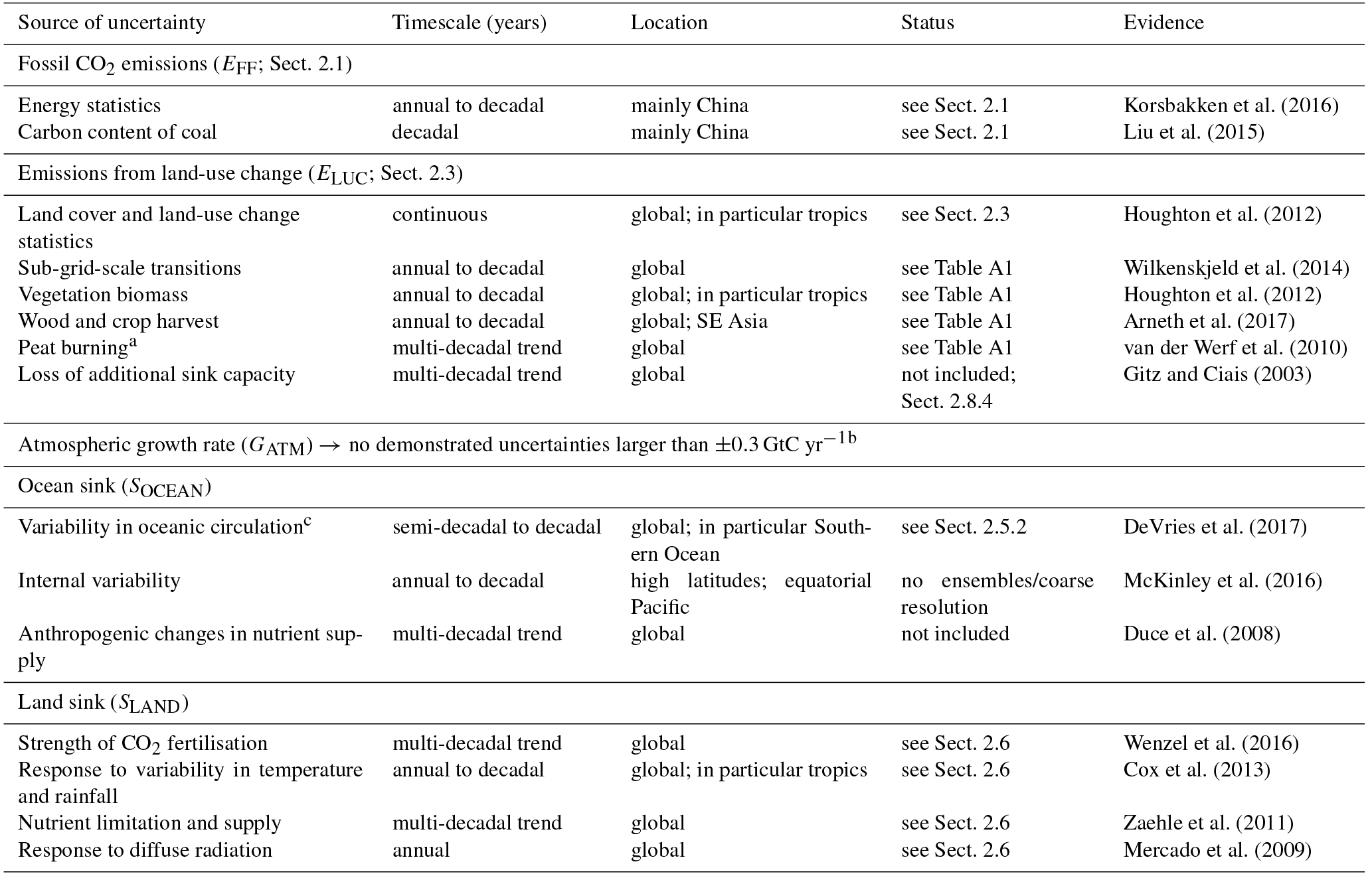
a As a result of interactions between land use and
climate.
b The uncertainties in GATM have been estimated as ±0.2 GtC yr−1, although the conversion of the growth rate into a
global
annual flux assuming instantaneous mixing throughout the atmosphere
introduces additional errors that have not yet been quantified.
c Could in part be due to uncertainties in
atmospheric forcing
(Swart et al., 2014).
Emissions were partitioned among the atmosphere (250±5 GtC), ocean (150±20 GtC), and the land (190±50 GtC). The use of nearly independent estimates for the individual terms shows a cumulative budget imbalance of 25 GtC during 1870–2017 (Fig. 2), which, if correct, suggests emissions are too high by the same proportion or the land or ocean sinks are underestimated. The bulk of the imbalance is likely to originate largely from the large estimation of ELUC between the mid-1920s and the mid-1960s, which is unmatched by a growth in atmospheric CO2 concentration as recorded in ice cores (Fig. 3). The known loss of additional sink capacity of about 20 GtC due to reduced forest cover has not been accounted for in our method and would further exacerbate the budget imbalance (Sect. 2.8.4). Cumulative emissions through to the year 2018 increase to 625±80 GtC (2290±290 GtCO2), with about a 70 % contribution from EFF and about a 30 % contribution from ELUC. Cumulative emissions and their partitioning for different periods are provided in Table 8.
Given the large and persistent uncertainties in cumulative emissions, we suggest extreme caution is needed if using cumulative emission estimates to determine the remaining carbon budget to stay below the given temperature limit (Rogelj et al., 2016). We suggest estimating the remaining carbon budget by integrating scenario data from the current time to some time in the future (Millar et al., 2017).
Each year when the global carbon budget is published, each flux component is updated for all previous years to consider corrections that are the result of further scrutiny and verification of the underlying data in the primary input data sets. Annual estimates may improve with improvements in data quality and timeliness (e.g. to eliminate the need for extrapolation of forcing data such as land use). Of the various terms in the global budget, only the fossil CO2 emissions and the growth rate in atmospheric CO2 concentration are based primarily on empirical inputs supporting annual estimates in this carbon budget. Although it is an imperfect measure, the carbon budget imbalance provides a strong indication of the limitations in observations, in understanding or full representation of processes in models, and/or in the integration of the carbon budget components.
The persistent unexplained variability in the carbon budget imbalance limits our ability to verify reported emissions (Peters et al., 2017) and suggests we do not yet have a complete understanding of the underlying carbon cycle processes. Resolving most of this unexplained variability should be possible through different and complementary approaches. First, as intended with our annual updates, the imbalance as an error term is reduced by improvements of individual components of the global carbon budget that follow from improving the underlying data and statistics and by improving the models through the resolution of some of the key uncertainties detailed in Table 9. Second, additional clues to the origin and processes responsible for the current imbalance could be obtained through a closer scrutiny of carbon variability in light of other Earth system data (e.g. heat balance, water balance), and the use of a wider range of biogeochemical observations to better understand the land–ocean partitioning of the carbon imbalance (e.g. oxygen, carbon isotopes). Finally, additional information could also be obtained through higher resolution and process knowledge at the regional level and through the introduction of inferred fluxes such as those based on satellite CO2 retrievals. The limit of the resolution of the carbon budget imbalance is yet unclear but most certainly not yet reached given the possibilities for improvements that lie ahead.
The assessment of the GOBMs used for SOCEAN with flux products based on observations highlights substantial discrepancy at mid-latitudes and high latitudes. Given the good data coverage of pCO2 observations in the Northern Hemisphere (Bakker et al., 2016), this discrepancy points to an underestimation of variability in the GOBMs globally, and consequently the variability in SOCEAN appears to be underestimated. The size of this underestimate (order of 0.5 GtC yr−1) could account for some of the budget imbalance, but not all. Increasing model resolution and incorporating internal variability (Li and Ilyina, 2018) have been suggested as ways to increase model variability (Sect. 3.1.4).
The assessment of the net land–atmosphere exchange derived from land sink and net land use change flux with atmospheric inversions also shows substantial discrepancy, particularly for the estimate of the total land flux over the northern extra-tropics in the past decade. This discrepancy highlights the difficulty to quantify complex processes (CO2 fertilisation, nitrogen deposition, climate change and variability, land management, etc.) that collectively determine the net land CO2 flux. Resolving the differences in the Northern Hemisphere land sink will require the consideration and inclusion of larger volumes of observations (Sect. 3.2.3).
Estimates of ELUC suffer from a range of intertwined issues, including the poor quality of historical land cover and land-use change maps, the rudimentary representation of management processes in most models, and the confusion in methodologies and boundary conditions used across methods (e.g. Pongratz et al., 2014; Arneth et al., 2017, and Sect. 2.8.4 on the loss of sink capacity). Uncertainties in current and historical carbon stocks in soils and vegetation also add uncertainty in the land-use change flux estimates. Unless a major effort to resolve these issues is made, little progress is expected in the resolution of ELUC. This is particularly concerning given the growing importance of ELUC for climate mitigation strategies and the large issues in the quantification of the cumulative emissions over the historical period that arise from large uncertainties in ELUC.
To move towards the resolution of the carbon budget imbalance, this year we have introduced metrics for the evaluation of the ocean and land models and atmospheric inversions. These metrics expand the use of observations in the global carbon budget, helping (1) to support improvements in the ocean and land carbon models that produce the sink estimates and (2) to constrain the representation of key underlying processes in the models and to allocate the regional partitioning of the CO2 fluxes. This is an initial step towards the introduction of a broader range of observations that we hope will support continued improvements in the annual estimates of the global carbon budget.
We assessed elsewhere (Peters et al., 2017) that a sustained decrease of −1 % in global emissions could be detected at the 66 % likelihood level after a decade only. Similarly, a change in behaviour of the land and/or ocean carbon sink would take as long to detect, and much longer if it emerges more slowly. Reducing the carbon imbalance, regionalising the carbon budget, and integrating multiple variables are powerful ways to shorten the detection limit and ensure the research community can rapidly identify growing issues of concern in the evolution of the global carbon cycle under the current rapid and unprecedented changing environmental conditions.
The data presented here are made available in the belief that their wide dissemination will lead to greater understanding and new scientific insights into how the carbon cycle works, how humans are altering it, and how we can mitigate the resulting human-driven climate change. The free availability of these data does not constitute permission for publication of the data. For research projects, if the data are essential to the work, or if an important result or conclusion depends on the data, co-authorship may need to be considered. Full contact details and information on how to cite the data shown here are given at the top of each page in the accompanying database and summarised in Table 2.
The accompanying database includes two Excel files organised in the following spreadsheets (accessible with the free viewer https://support.microsoft.com/en-gb/help/273711/how-to-obtain-the-latest-excel-viewer, last access: 28 November 2018):
File Global_Carbon_Budget_2018v1.0.xlsx (Global Carbon Project, 2018) includes the following:
-
summary;
-
the global carbon budget (1959–2017),
-
global CO2 emissions from fossil fuels and cement production by fuel type and the per capita emissions (1959–2017),
-
CO2 emissions from land-use change from the individual methods and models (1959–2017),
-
ocean CO2 sink from the individual ocean models and pCO2-based products (1959–2017),
-
terrestrial CO2 sink from the DGVMs (1959–2017),
-
additional information on the carbon balance prior to 1959 (1750–2017).
File National_Carbon_Emissions_2018v1.0.xlsx (Global Carbon Project, 2018) includes the following:
-
summary
-
territorial country CO2 emissions from fossil CO2 emissions (1959–2017) from CDIAC with UNFCCC data overwritten where available, extended to 2017 using BP data;
-
consumption country CO2 emissions from fossil CO2 emissions and emission transfer from the international trade of goods and services (1990–2016) using CDIAC/UNFCCC data (worksheet 3 above) as reference;
-
emission transfers (consumption minus territorial emissions; 1990–2016);
-
country definitions;
-
details of disaggregated countries;
-
details of aggregated countries.
National emission data are also available from the Global Carbon Atlas (http://www.globalcarbonatlas.org/, last access: 28 November 2018).
The estimation of global CO2 emissions and sinks is a major effort by the carbon cycle research community that requires a careful compilation and synthesis of measurements, statistical estimates, and model results. The delivery of an annual carbon budget serves two purposes. First, there is a large demand for up-to-date information on the state of the anthropogenic perturbation of the climate system and its underpinning causes. A broad stakeholder community relies on the data sets associated with the annual carbon budget including scientists, policymakers, businesses, journalists, and non-governmental organisations engaged in adapting to and mitigating human-driven climate change. Second, over the last decade we have seen unprecedented changes in the human and biophysical environments (e.g. changes in the growth of fossil fuel emissions, Earth's temperatures, and strength of the carbon sinks), which call for frequent assessments of the state of the planet and a growing understanding of and improved capacity to anticipate the evolution of the carbon cycle in the future. Building this scientific understanding to meet the extraordinary climate mitigation challenge requires frequent, robust, and transparent data sets and methods that can be scrutinised and replicated. This paper via living data helps to keep track of new budget updates.
Table A1Comparison of the processes included (Y) or not (N) in the bookkeeping and dynamic global vegetation models for their estimates of ELUC and SLAND. See Table 4 for model references. All models include deforestation and forest regrowth after abandonment of agriculture (or from afforestation activities on agricultural land).
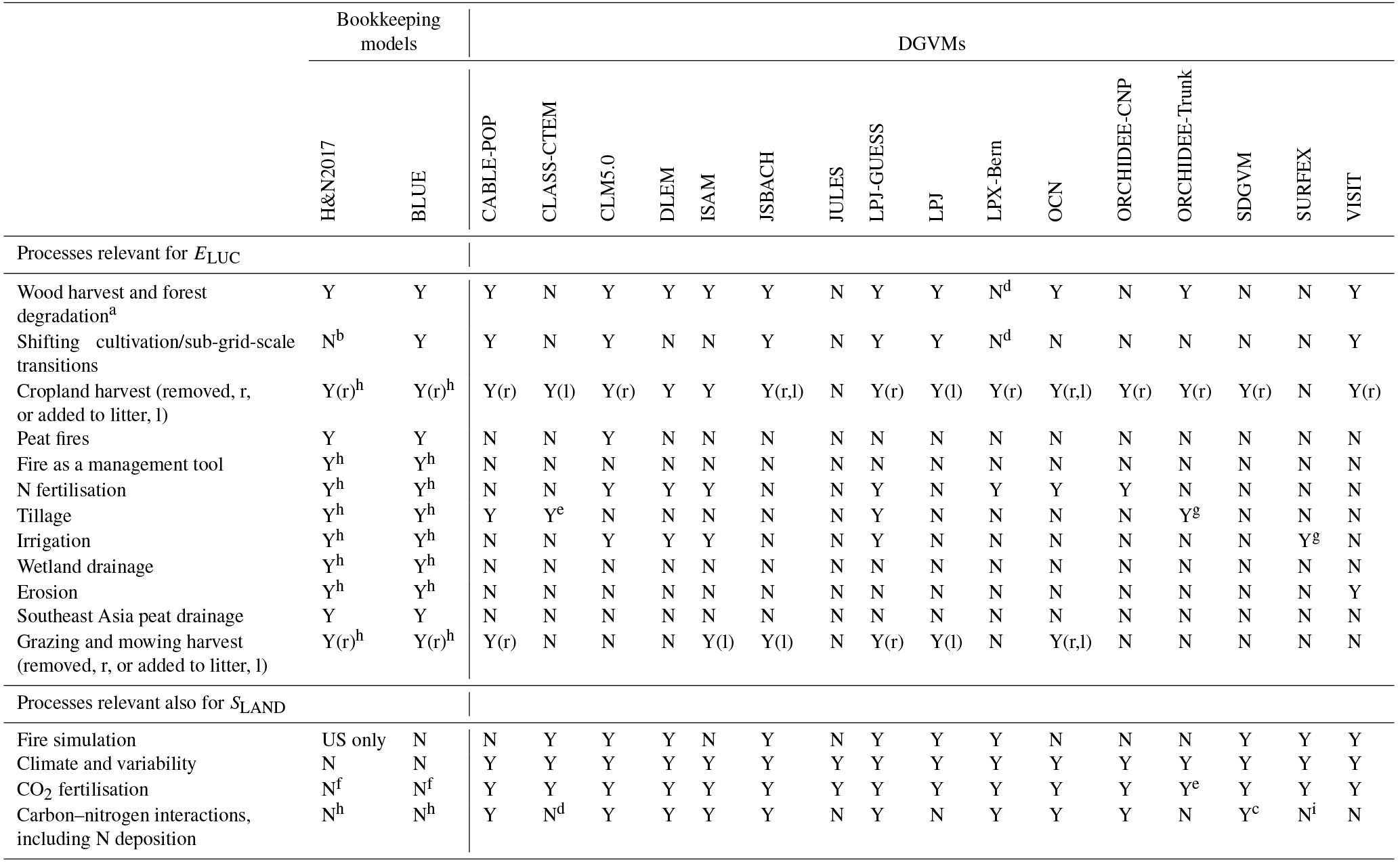
a Refers to the routine harvest of established managed forests rather
than pools of harvested products.
b No back-and-forth transitions between vegetation types at the
country level,
but if forest loss based on FRA exceeded agricultural
expansion based on the FAO, then this amount of area is interpreted as shifting
cultivation.
c Limited. Nitrogen uptake is simulated
as a function of soil C, and
photosynthesis is directly related to canopy N. Does not consider N
deposition.
d Although C–N cycle interactions are not represented, the model
includes
a parameterization of down-regulation of photosynthesis as
CO2 increases to emulate nutrient constraints
(Arora et al., 2009).
e Tillage is represented over croplands by increased
soil carbon
decomposition rate and reduced humification of litter to soil carbon.
f Bookkeeping models include the effect of CO2 fertilisation as
captured by observed carbon densities,
but not as an effect that is transient in
time.
g A 20 % reduction of active soil organic carbon (SOC) pool turnover
time for C3 crops and 40 % reduction for C4 crops.
h Process captured
implicitly by use of observed carbon densities.
i Simple parameterization of nitrogen limitation based on Yin
(2002; assessed on FACE experiments).
Table A2Comparison of the processes and model set-up for the global ocean biogeochemistry models for their estimates of SOCEAN. See Table 4 for model references.
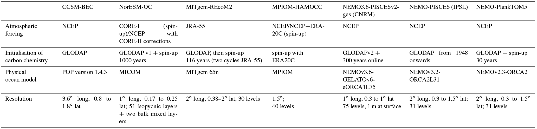
Table A3Comparison of the inversion set-up and input fields for the atmospheric inversions. Atmospheric inversions see the full CO2 fluxes, including the anthropogenic and pre-industrial fluxes. Hence they need to be adjusted for the pre-industrial flux of CO2 from the land to the ocean that is part of the natural carbon cycle before they can be compared with SOCEAN and SLAND from process models. See Table 4 for references.
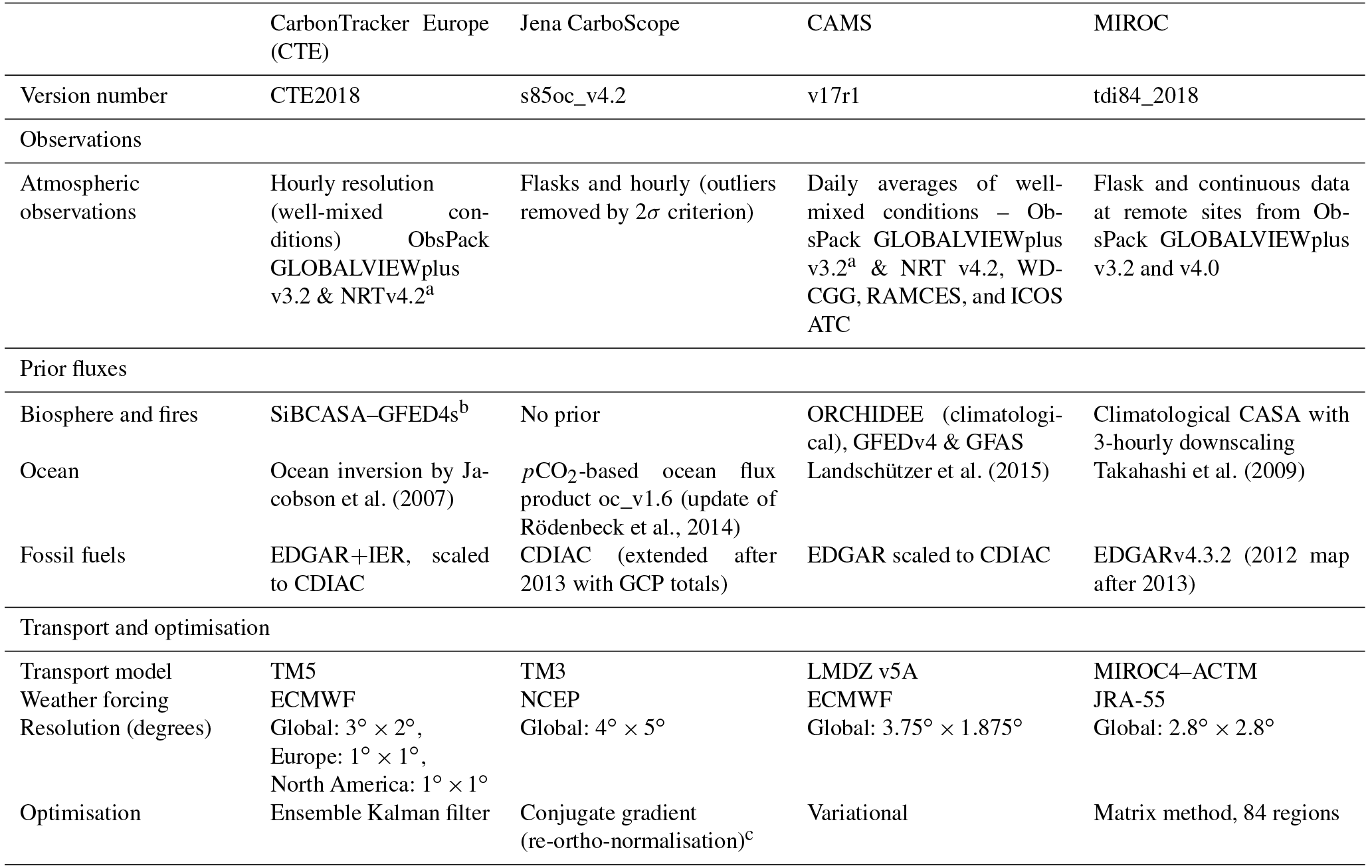
a GLOBALVIEW (2016); CarbonTracker Team (2017). b Van der Velde et al. (2014). c Ocean prior not optimised.
Table A4Attribution of fCO2 measurements for the year 2017 included in SOCAT v6 (Bakker et al., 2016) to inform ocean pCO2-based flux products.
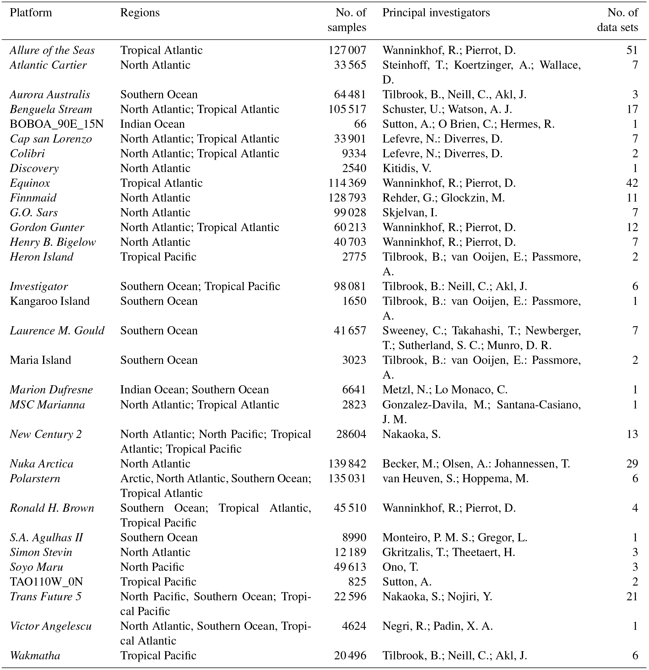
Table A5Funding supporting the production of the various components of the global carbon budget in addition to the authors' supporting institutions (see also acknowledgements).
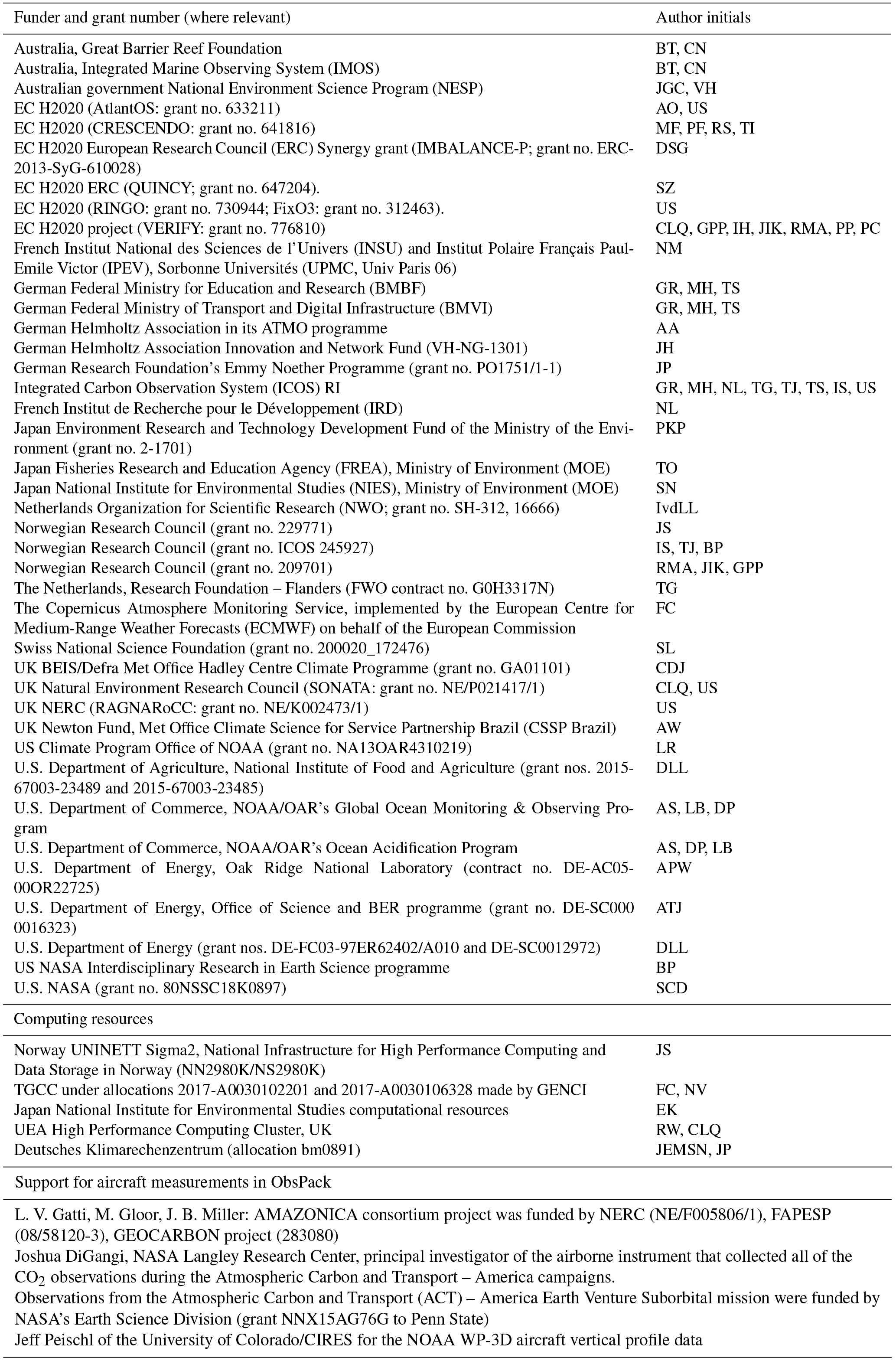
Table A6Aircraft measurement programmes archived by Cooperative Global Atmospheric Data Integration Project (CGADIP, 2017) that contribute to the evaluation of the atmospheric inversions (Fig. B3).
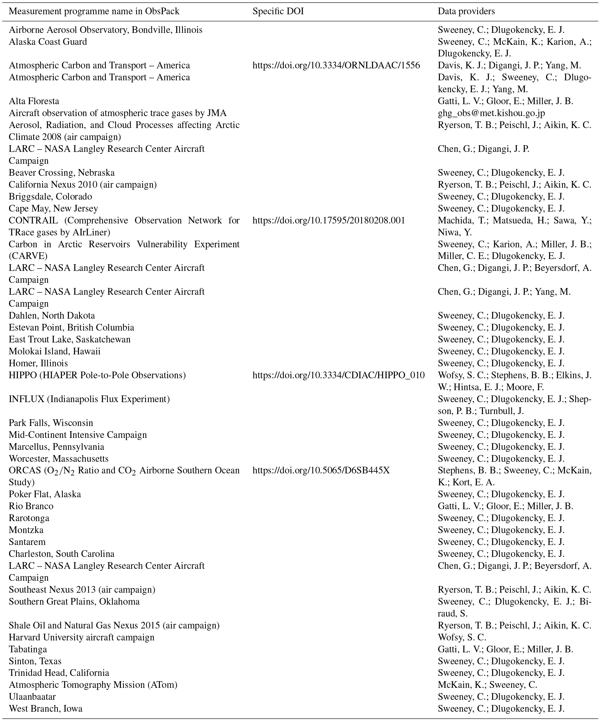
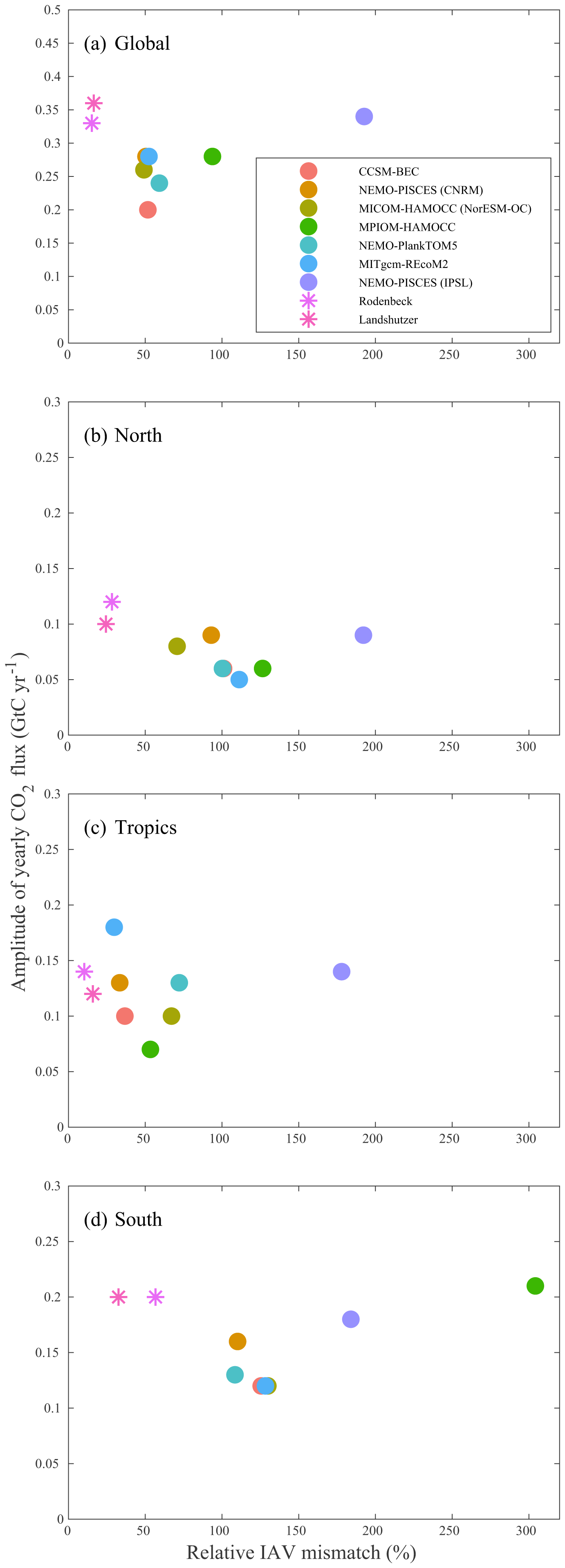
Figure B1Evaluation of the GOBMs and flux products using the interannual mismatch metric for the period from 1985 to 2017, as proposed by Rödenbeck et al. (2015) and the SOCAT v6 database, versus the amplitude of the annual variability (taken as the annual standard deviation). Results are presented for the globe, north (>30∘ N), tropics (30∘ S–30∘ N), and south (<30∘ S) for the GOBMs (circles) and for the pCO2-based flux products (star symbols). The two pCO2-based flux products use the SOCAT database and therefore are not fully independent from the data (see Sect. 2.5.1).
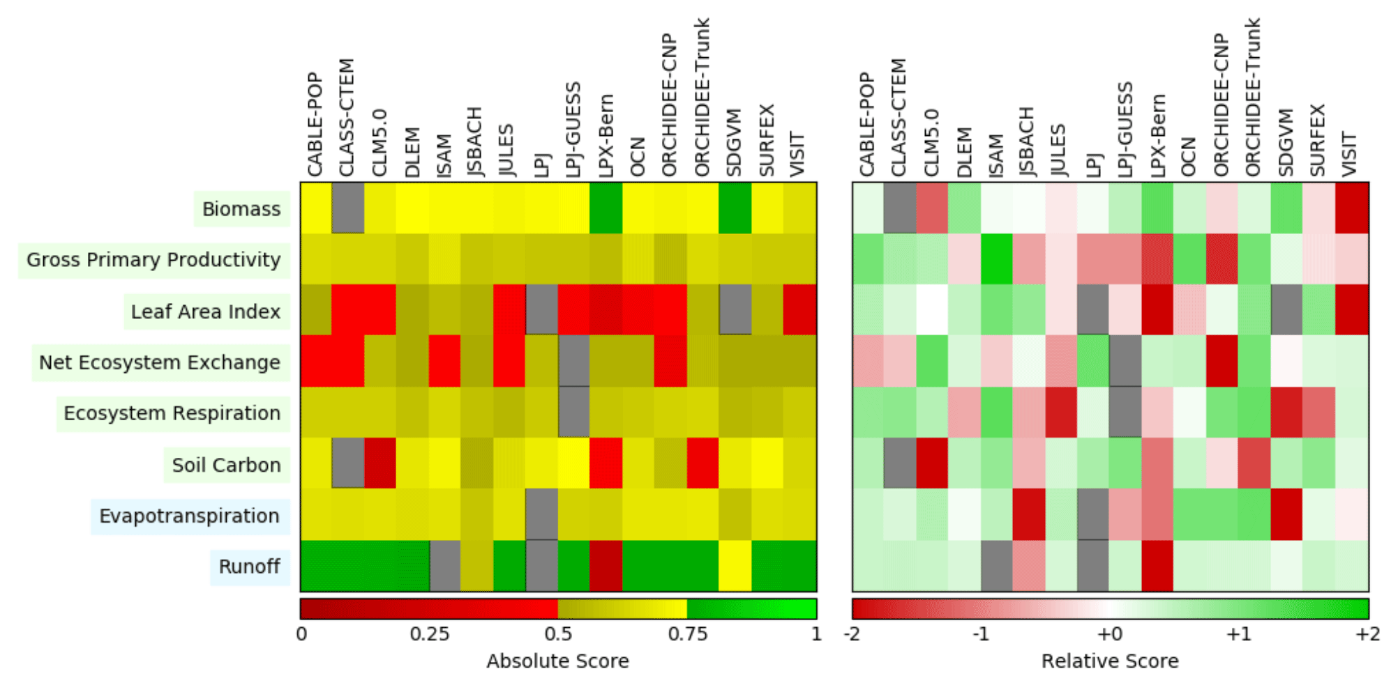
Figure B2Evaluation of the DGVM using the International Land Model Benchmarking system (ILAMB; Collier et al., 2018) (left) absolute skill scores and (right) skill scores relative to other models. The benchmarking is carried out with observations for vegetation biomass (Saatchi et al., 2011; GlobalCarbon, unpublished data; Avitabile et al., 2016), GPP (Jung et al., 2010; Lasslop et al., 2010), leaf area index (De Kauwe et al., 2011; Myneni et al., 1997), net ecosystem exchange (Jung et al., 2010; Lasslop et al., 2010), ecosystem respiration (Jung et al., 2010; Lasslop et al., 2010), soil carbon (Hugelius et al., 2013; Todd-Brown et al., 2013), evapotranspiration (De Kauwe et al., 2011), and runoff (Dai and Trenberth, 2002). For each model–observation comparison a series of error metrics are calculated, scores are then calculated as an exponential function of each error metric, and finally for each variable the multiple scores from different metrics and observational data sets are combined to give the overall variable scores shown in the left panel. The set of error metrics vary with data set and can include metrics based on the period mean, bias, root-mean-squared error, spatial distribution, interannual variability, and seasonal cycle. The relative skill score shown in the right panel is a Z score, which indicates in units of standard deviation the model scores relative to the multi-model mean score for a given variable. Grey boxes represent missing model data.
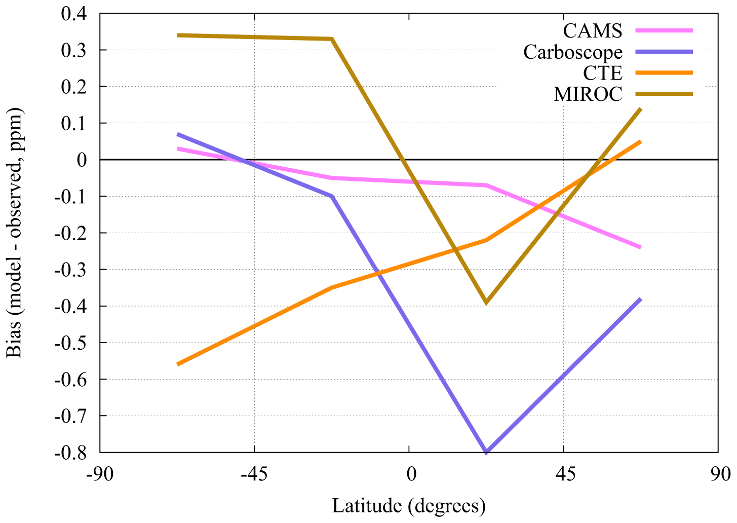
Figure B3Evaluation of the atmospheric inversion products. The mean of the absolute model minus observations is shown for four latitude bands. The four models are compared to independent CO2 measurements made onboard aircraft over many places of the world between 1 and 7 km above sea level. All data between 2008 and 2016 archived in the Cooperative Global Atmospheric Data Integration Project (CGADIP, 2017) have been used to compute the biases of the differences in four 45∘ latitude bins. Land and ocean data are used without distinction. The number of data for each latitude band is 16 000 (90–45∘ S), 53 000 (45∘ S–0), 64 000 (0–45∘ N), and 122 000 (45–90∘ N), rounded off to the nearest thousand.
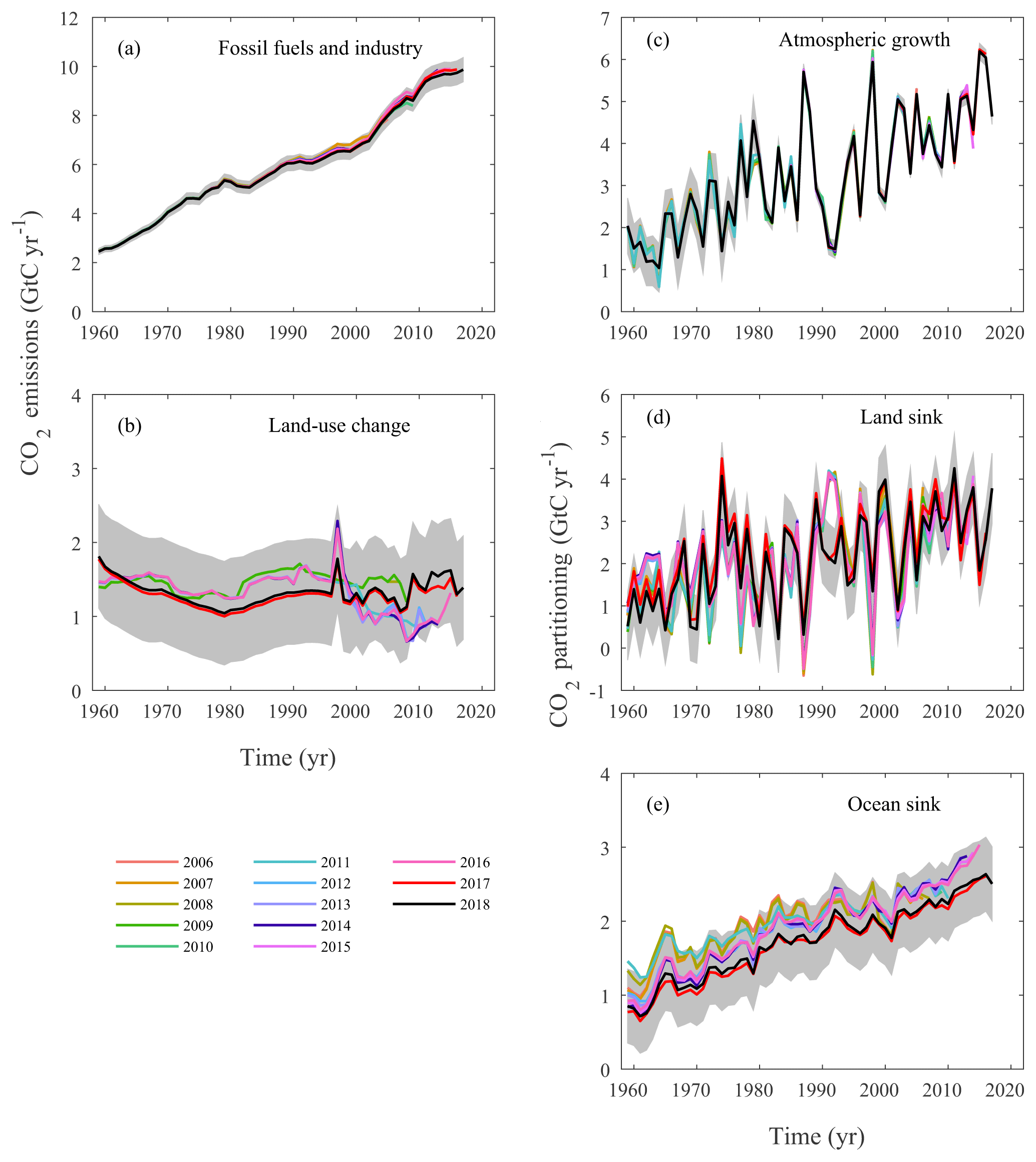
Figure B4Comparison of global carbon budget components released annually by GCP since 2006. CO2 emissions from (a) fossil CO2 emissions (EFF) and (b) land-use change (ELUC), as well as their partitioning among (c) the atmosphere (GATM), (d) the land (SLAND), and (e) the ocean (SOCEAN). See legend for the corresponding years and Table 3 for references. The budget year corresponds to the year when the budget was first released. All values are in GtC yr−1. Grey shading shows the uncertainty bounds representing ±1σ of the current global carbon budget.
CLQ, RMA, PF, SS, JH, JP, GPP, JGC, and WP designed the study, conducted the analysis, and wrote the paper. RMA and GPP produced the emissions and their uncertainties, 2018 emission projections, and analysed the emissions data. RMA, JIK, GPP, ZL, and BZ produced the 2018 projection for China's emissions and its uncertainty. RFK and PPT provided key atmospheric CO2 data. RMA and CDJ produced the 2018 projection for atmospheric CO2 growth rate and its uncertainty. FC, PPa, CR, and IvdLL provided an updated atmospheric inversion, developed the protocol and produced the evaluation. AB and RAH provided updated land-use change emissions. LPC, GH, KKG, FNT, and GRvdW provided forcing data for land-use change. AA, VKA, DSG, VH, AKJ, EK, SL, DL, JEMSN, PPe, BPo, MR, HT, APW, AJW and SZ provided an update of a DGVM. IH and NV provided forcing data for the DGVMs. FMH and ER provided the evaluation of the DGVMs. JH, LBo, SCD, TI, JS, RS and RW provided an update of a GOBM. PL and CR provided an update of an ocean flux product. Lba, TG, MH, TJ, NL, NM, DRM, SN, CN, AO, TO, BPf, DP, GR, US, IS, TS, AS and BT provided ocean pCO2 measurements for the year 2017. LR provided an updated river flux estimate. CLQ, PAP, RMA and AP revised the figures, tables, text and/or numbers to ensure the update is clear from the 2017 edition and in phase with the globalcarbonatlas.org.
The authors declare that they have no conflict of interest.
We thank all people and institutions who provided the data used in this carbon budget; Richard Betts, Erik Buitenhuis, Jinfeng Chang, Shijie Shu, and Naomi Smith for their involvement in the development, use and analysis of the models and data products used here; and Fortunat Joos, Samar Khatiwala, and Timothy DeVries for providing historical data. We thank Rob Jackson and the Global Carbon Project members for their input throughout the development of this update. We thank Ed Dlugokencky for providing atmospheric CO2 measurements; Camilla Stegen Landa, Christophe Bernard, and Steve Jones of the Bjerknes Climate Data Centre and the ICOS Ocean Thematic Centre data management at the University of Bergen, who helped with gathering information from the SOCAT community; and Vassilis Kitidis, Pedro M. S. Monteiro, Luke Gregor, Melchor Gonzáles-Dávila, J. Magdalena Santana-Casiano, Ruben Negri, and X. Antonio Padin, who contributed to the provision of ocean pCO2 observations (see Table A1). This is NOAA-PMEL contribution number 4847. We thank the institutions and funding agencies responsible for the collection and quality control of the data included in SOCAT and the support of the International Ocean Carbon Coordination Project (IOCCP), the Surface Ocean–Lower Atmosphere Study (SOLAS), and the Integrated Marine Biogeochemistry and Ecosystem Research (IMBER) programme. We thank the FAO and its member countries for the collection and free dissemination of data relevant to this work. We thank data providers ObsPack GLOBALVIEWplus v1.0 and NRT v3.0 for atmospheric CO2 observations used in CTE2016-FT and the following people for sharing their aircraft data used in Fig. B3: Toshinobu Machida, Guangsheng Chen, Steven C. Wofsy, Ken Davis, Joshua DiGangi, Jeff Peischl, Thomas B. Ryerson, Britton Stephens, Colm Sweeney, Kathryn McKain, and Luciana V. Gatti; University of Colorado/CIRES for the NOAA WP-3D aircraft vertical profile data; and the Japan Meteorological Agency. We thank the individuals and institutions that provided the databases used for the model evaluations introduced here and Nigel Hawtin for producing Fig. 2.
Finally, we thank all funders who have supported the individual and joint
contributions to this work (see Table A5), as well as the reviewers of this
paper and previous versions, and the many researchers who have provided
feedback.
Edited by: David Carlson
Reviewed by: H. Damon Matthews, Albertus J. Dolman,
and one
anonymous referee
Andres, R. J., Boden, T. A., Bréon, F.-M., Ciais, P., Davis, S., Erickson, D., Gregg, J. S., Jacobson, A., Marland, G., Miller, J., Oda, T., Olivier, J. G. J., Raupach, M. R., Rayner, P., and Treanton, K.: A synthesis of carbon dioxide emissions from fossil-fuel combustion, Biogeosciences, 9, 1845–1871, https://doi.org/10.5194/bg-9-1845-2012, 2012.
Andres, R. J., Boden, T., and Higdon, D.: A new evaluation of the uncertainty associated with CDIAC estimates of fossil fuel carbon dioxide emission, Tellus B, 66, 23616, https://doi.org/10.3402/tellusb.v66.23616, 2014.
Andrew, R. M.: Global CO2 emissions from cement production, Earth Syst. Sci. Data, 10, 195–217, https://doi.org/10.5194/essd-10-195-2018, 2018.
Andrew, R. M. and Peters, G. P.: A multi-region input-output table based on the Global Trade Analysis Project Database (GTAP-MRIO), Econ. Syst. Res., 25, 99–121, https://doi.org/10.1080/09535314.2012.761953, 2013.
Archer, D., Eby, M., Brovkin, V., Ridgwell, A., Cao, L., Mikolajewicz, U., Caldeira, K. M., K., Munhoven, G., Montenegro, A., and Tokos, K.: Atmospheric Lifetime of Fossil Fuel Carbon Dioxide, Annu. Rev. Earth Pl. Sc., 37, 117–134, https://doi.org/10.1146/annurev.earth.031208.100206, 2009.
Arneth, A., Sitch, S., Pongratz, J., Stocker, B. D., Ciais, P., Poulter, B., Bayer, A. D., Bondeau, A., Calle, L., Chini, L. P., Gasser, T., Fader, M., Friedlingstein, P., Kato, E., Li, W., Lindeskog, M., Nabel, J. E. M. S., Pugh, T. A. M., Robertson, E., Viovy, N., Yue, C., and Zaehle, S.: Historical carbon dioxide emissions caused by land-use changes are possibly larger than assumed, Nat. Geosci., 10, 79–84, https://doi.org/10.1038/ngeo2882, 2017.
Arora, V. K., Boer, G. J., Christian, J. R., Curry, C. L., Denman, K. L., Zahariev, K., Flato, G. M., Scinocca, J. F., Merryfield, W. J., and Lee, W. G.: The Effect of Terrestrial Photosynthesis Down Regulation on the Twentieth-Century Carbon Budget Simulated with the CCCma Earth System Model, J. Climate, 22, 6066–6088, https://doi.org/10.1175/2009jcli3037.1, 2009.
Aumont, O. and Bopp, L.: Globalizing results from ocean in situ iron fertilization studies, Global Biogeochem. Cy., 20, GB2017, https://doi.org/10.1029/2005GB002591, 2006.
Avitabile, V., Herold, M., Heuvelink, G. B. M., Lewis, S. L., Phillips, O. L., Asner, G. P., Armston, J., Ashton, P. S., Banin, L., Bayol, N., Berry, N. J., Boeckx, P., de Jong, B. H. J., DeVries, B., Girardin, C. A. J., Kearsley, E., Lindsell, J. A., Lopez-Gonzalez, G., Lucas, R., Malhi, Y., Morel, A., Mitchard, E. T. A., Nagy, L., Qie, L., Quinones, M. J., Ryan, C. M., Ferry, S. J. W., Sunderland, T., Laurin, G. V., Gatti, R. C., Valentini, R., Verbeeck, H., Wijaya, A., and Willcock, S.: An integrated pan-tropical biomass map using multiple reference datasets, Glob. Change Biol., 22, 1406–1420, https://doi.org/10.1111/gcb.13139, 2016.
Baccini, A., Walker, W., Carvalho, L., Farina, M., Sulla-Menashe, D., and Houghton, R. A.: Tropical forests are a net carbon source based on aboveground measurements of gain and loss, Science, 358, 230–233, https://doi.org/10.1126/science.aam5962, 2017.
Bakker, D. C. E., Pfeil, B., Landa, C. S., Metzl, N., O'Brien, K. M., Olsen, A., Smith, K., Cosca, C., Harasawa, S., Jones, S. D., Nakaoka, S.-I., Nojiri, Y., Schuster, U., Steinhoff, T., Sweeney, C., Takahashi, T., Tilbrook, B., Wada, C., Wanninkhof, R., Alin, S. R., Balestrini, C. F., Barbero, L., Bates, N. R., Bianchi, A. A., Bonou, F., Boutin, J., Bozec, Y., Burger, E. F., Cai, W.-J., Castle, R. D., Chen, L., Chierici, M., Currie, K., Evans, W., Featherstone, C., Feely, R. A., Fransson, A., Goyet, C., Greenwood, N., Gregor, L., Hankin, S., Hardman-Mountford, N. J., Harlay, J., Hauck, J., Hoppema, M., Humphreys, M. P., Hunt, C. W., Huss, B., Ibánhez, J. S. P., Johannessen, T., Keeling, R., Kitidis, V., Körtzinger, A., Kozyr, A., Krasakopoulou, E., Kuwata, A., Landschützer, P., Lauvset, S. K., Lefèvre, N., Lo Monaco, C., Manke, A., Mathis, J. T., Merlivat, L., Millero, F. J., Monteiro, P. M. S., Munro, D. R., Murata, A., Newberger, T., Omar, A. M., Ono, T., Paterson, K., Pearce, D., Pierrot, D., Robbins, L. L., Saito, S., Salisbury, J., Schlitzer, R., Schneider, B., Schweitzer, R., Sieger, R., Skjelvan, I., Sullivan, K. F., Sutherland, S. C., Sutton, A. J., Tadokoro, K., Telszewski, M., Tuma, M., van Heuven, S. M. A. C., Vandemark, D., Ward, B., Watson, A. J., and Xu, S.: A multi-decade record of high-quality fCO2 data in version 3 of the Surface Ocean CO2 Atlas (SOCAT), Earth Syst. Sci. Data, 8, 383–413, https://doi.org/10.5194/essd-8-383-2016, 2016.
Ballantyne, A. P., Alden, C. B., Miller, J. B., Tans, P. P., and White, J. W. C.: Increase in observed net carbon dioxide uptake by land and oceans during the last 50 years, Nature, 488, 70–72, https://doi.org/10.1038/nature11299, 2012.
Ballantyne, A. P., Andres, R., Houghton, R., Stocker, B. D., Wanninkhof, R., Anderegg, W., Cooper, L. A., DeGrandpre, M., Tans, P. P., Miller, J. B., Alden, C., and White, J. W. C.: Audit of the global carbon budget: estimate errors and their impact on uptake uncertainty, Biogeosciences, 12, 2565–2584, https://doi.org/10.5194/bg-12-2565-2015, 2015.
Bauer, J. E., Cai, W.-J., Raymond, P. A., Bianchi, T. S., Hopkinson, C. S., and Regnier, P. A. G.: The changing carbon cycle of the coastal ocean, Nature, 504, 61–70, https://doi.org/10.1038/nature12857, 2013.
Berthet, S., Séférian, R., Bricaud, C., Chevallier, M., Voldoire, A., and Ethé, C.: On the benefits of increasing resolution for biogeochemistry climate modelling, J. Adv. Model. Earth Sy., submitted, 2018.
Betts, R. A., Jones, C. D., Knight, J. R., Keeling, R. F., and Kennedy, J. J.: El Nino and a record CO2 rise, Nat. Clim. Change, 6, 806–810, https://doi.org/10.1038/nclimate3063, 2016.
Boden, T. A., Marland, G., and Andres, R. J.: Global, Regional, and National Fossil-Fuel CO2 Emissions, available at: http://cdiac.ornl.gov/trends/emis/overview_2014.html (last access: July 2017), Oak Ridge National Laboratory, U.S. Department of Energy, Oak Ridge, Tenn., USA, 2017.
BP: BP Statistical Review of World Energy June 2018, available at: https://www.bp.com/content/dam/bp/en/corporate/pdf/energy-economics/statistical-review/bp-stats-review-2018-full-report.pdf, last access: June 2018.
Bruno, M. and Joos, F.: Terrestrial carbon storage during the past 200 years: A monte carlo analysis of CO2 data from ice core and atmospheric measurements, Global Biogeochem. Cy., 11, 111–124, https://doi.org/10.1029/96GB03611, 1997.
Buitenhuis, E. T., Rivkin, R. B., Sailley, S., and Le Quéré, C.: Biogeochemical fluxes through microzooplankton, Global Biogeochem. Cy., 24, GB4015, https://doi.org/10.1029/2009GB003601, 2010.
Canadell, J. G., Le Quéré, C., Raupach, M. R., Field, C. B., Buitenhuis, E. T., Ciais, P., Conway, T. J., Gillett, N. P., Houghton, R. A., and Marland, G.: Contributions to accelerating atmospheric CO2 growth from economic activity, carbon intensity, and efficiency of natural sinks, P. Natl. Acad. Sci. USA, 104, 18866–18870, https://doi.org/10.1073/pnas.0702737104, 2007.
Carbontracker Team: Compilation of near real time atmospheric carbon dioxide data provided by NOAA and EC, obspack_co2_1_NRT_v3.3_2017-04-19; NOAA Earth System Research Laboratory, Global Monitoring Division, https://doi.org/10.15138/G3G01J, 2017.
CEA: Central Electricity Authority (CEA), 2018: Daily Coal – Archive, Central Electricity Authority, available at: http://www.cea.nic.in/dailyarchive.html, last access: 7 November 2018.
CGADIP: Cooperative Global Atmospheric Data Integration Project (2017), Multi-laboratory compilation of atmospheric carbon dioxide data for the period 1957–2016; obspack_co2_1_GLOBALVIEWplus_v3.2_2017-11-02 [Data set], NOAA Earth System Research Laboratory, Global Monitoring Division, 2017.
Chatfield, C.: The Holt-Winters Forecasting Procedure, J. Roy. Stat. Soc. C-Appl., 27, 264–279, https://doi.org/10.2307/2347162, 1978.
Chevallier, F., Fisher, M., Peylin, P., Serrar, S., Bousquet, P., Bréon, F.-M., Chédin, A., and Ciais, P.: Inferring CO2 sources and sinks from satellite observations: Method and application to TOVS data, J. Geophys. Res., 110, D24309, https://doi.org/10.1029/2005JD006390, 2005.
Ciais, P., Sabine, C., Govindasamy, B., Bopp, L., Brovkin, V., Canadell, J., Chhabra, A., DeFries, R., Galloway, J., Heimann, M., Jones, C., Le Quéré, C., Myneni, R., Piao, S., and Thornton, P.: Chapter 6: Carbon and Other Biogeochemical Cycles, in: Climate Change 2013 The Physical Science Basis, edited by: Stocker, T., Qin, D., and Platner, G.-K., Cambridge University Press, Cambridge, 2013.
CIL: Coal India Limited, 2018: Production and Offtake Performance of CIL and Subsidiary Companies, available at: https://www.coalindia.in/en-us/performance/physical.aspx, last access: 1 November 2018.
Clark, D. B., Mercado, L. M., Sitch, S., Jones, C. D., Gedney, N., Best, M. J., Pryor, M., Rooney, G. G., Essery, R. L. H., Blyth, E., Boucher, O., Harding, R. J., Huntingford, C., and Cox, P. M.: The Joint UK Land Environment Simulator (JULES), model description – Part 2: Carbon fluxes and vegetation dynamics, Geosci. Model Dev., 4, 701–722, https://doi.org/10.5194/gmd-4-701-2011, 2011.
Collier, N., Hoffman, F. M., Lawrence, D. M., Keppel-Aleks, G., Koven, C. D., Riley, W. J., Mu, M., and Randerson, J. T.: The International Land Model Benchmarking (ILAMB) System: Design, Theory, and Implementation, J. Adv. Model. Earth Sy., 10, https://doi.org/10.1029/2018MS001354, 2018.
Cox, P. M., Pearson, D., Booth, B. B., Friedlingstein, P., Huntingford, C., Jones, C. D., and Luke, C. M.: Sensitivity of tropical carbon to climate change constrained by carbon dioxide variability, Nature, 494, 341–344, https://doi.org/10.1038/nature11882, 2013.
Dai, A. and Trenberth, K. E.: Estimates of freshwater discharge from continents: Latitudinal and seasonal variations, J. Hydrometeorol., 3, 660–687, https://doi.org/10.1175/1525-7541(2002)003<0660:EOFDFC>2.0.CO;2, 2002.
Davis, S. J. and Caldeira, K.: Consumption-based accounting of CO2 emissions, P. Natl. Acad. Sci. USA, 107, 5687–5692, https://doi.org/10.1073/pnas.0906974107, 2010.
De Kauwe, M. G., Disney, M. I., Quaife, T., Lewis, P., and Williams, M.: An assessment of the MODIS collection 5 leaf area index product for a region of mixed coniferous forest, Remote Sens. Environ., 115, 767–780, https://doi.org/10.1016/j.rse.2010.11.004, 2011.
Denman, K. L., Brasseur, G., Chidthaisong, A., Ciais, P., Cox, P. M., Dickinson, R. E., Hauglustaine, D., Heinze, C., Holland, E., Jacob, D., Lohmann, U., Ramachandran, S., Leite da Silva Dias, P., Wofsy, S. C., and Zhang, X.: Couplings Between Changes in the Climate System and Biogeochemistry, in: Climate Change 2007: The Physical Science Basis. Contribution of Working Group I to the Fourth Assessment Report of the Intergovernmental Panel on Climate Change, edited by: Solomon, S., Qin D., Manning M., Marquis M., Averyt K., Tignor M. M. B., Miller, H. L., and Chen Z. L., Cambridge University Press, Cambridge, UK and New York, USA, 499–587, 2007.
DeVries, T.: The oceanic anthropogenic CO2 sink: Storage, air-sea fluxes, and transports over the industrial era, Global Biogeochem. Cy., 28, 631–647, https://doi.org/10.1002/2013GB004739, 2014.
DeVries, T., Holzer, M., and Primeau, F.: Recent increase in oceanic carbon uptake driven by weaker upper-ocean overturning, Nature, 542, 215–218, https://doi.org/10.1038/nature21068, 2017.
Dlugokencky, E. and Tans, P.: Trends in atmospheric carbon dioxide, National Oceanic & Atmospheric Administration, Earth System Research Laboratory (NOAA/ESRL), available at: http://www.esrl.noaa.gov/gmd/ccgg/trends/global.html, last access: 4 September 2018.
Doney, S. C., Lima, I., Feely, R. A., Glover, D. M., Lindsay, K., Mahowald, N., Moore, J. K., and Wanninkhof, R.: Mechanisms governing interannual variability in upper-ocean inorganic carbon system and air–sea CO2 fluxes: Physical climate and atmospheric dust, Deep-Sea Res. Pt. II, 56, 640–655, https://doi.org/10.1016/j.dsr2.2008.12.006, 2009.
Duce, R. A., LaRoche, J., Altieri, K., Arrigo, K. R., Baker, A. R., Capone, D. G., Cornell, S., Dentener, F., Galloway, J., Ganeshram, R. S., Geider, R. J., Jickells, T., Kuypers, M. M., Langlois, R., Liss, P. S., Liu, S. M., Middelburg, J. J., Moore, C. M., Nickovic, S., Oschlies, A., Pedersen, T., Prospero, J., Schlitzer, R., Seitzinger, S., Sorensen, L. L., Uematsu, M., Ulloa, O., Voss, M., Ward, B., and Zamora, L.: Impacts of atmospheric anthropogenic nitrogen on the open ocean, Science, 320, 893–897, https://doi.org/10.1126/science.1150369, 2008.
Dufour, C. O., Le Sommer, J., Gehlen, M., Orr, J. C., Molines, J. M., Simeon, J., and Barnier, B.: Eddy compensation and controls of the enhanced sea-to-air CO2 flux during positive phases of the Southern Annular Mode, Global Biogeochem. Cy., 27, 950–961, https://doi.org/10.1002/gbc.20090, 2013.
Durant, A. J., Le Quéré, C., Hope, C., and Friend, A. D.: Economic value of improved quantification in global sources and sinks of carbon dioxide, Philos. T. Roy Soc. A, 269, 1967–1979, https://doi.org/10.1098/rsta.2011.0002, 2011.
EIA: U.S. Energy Information Administration, Short-Term Energy and Winter Fuels Outlook, available at: http://www.eia.gov/forecasts/steo/outlook.cfm, last access: 7 November 2018.
ENTSO-E: The European Network of Transmission System Operators Electricity Transparency Platform, available at: https://transparency.entsoe.eu/, last access: 1 November 2018.
Erb, K.-H., Kastner, T., Luyssaert, S., Houghton, R. A., Kuemmerle, T., Olofsson, P., and Haberl, H.: Bias in the attribution of forest carbon sinks, Nat. Clim. Change, 3, 854–856, https://doi.org/10.1038/nclimate2004, 2013.
Etheridge, D. M., Steele, L. P., Langenfelds, R. L., and Francey, R. J.: Natural and anthropogenic changes in atmospheric CO2 over the last 1000 years from air in Antarctic ice and firn, J. Geophys. Res., 101, 4115–4128, https://doi.org/10.1029/95JD03410, 1996.
Eurostat: Supply and transformation of solid fuels – monthly data (nrg_101m), available at: https://ec.europa.eu/eurostat/data/database, last access: 7 November 2018.
FAO: Global Forest Resources Assessment 2015, Food and Agriculture Organization of the United Nations, Rome, Italy, 2015.
FAOSTAT: Food and Agriculture Organization Statistics Division, available at: http://faostat.fao.org/, last access: 2015.
Figueres, C., Whiteman, G., Le Quéré, C., and Peters, G. P.: Carbon emissions rise again, Nature, 564, 27–31, 2018.
Francey, R. J., Trudinger, C. M., van der Schoot, M., Law, R. M., Krummel, P. B., Langenfelds, R. L., Steele, L. P., Allison, C. E., Stavert, A. R., Andres, R. J., and Rodenbeck, C.: Reply to “Anthropogenic CO2 emissions”, Nat. Clim. Change, 3, p. 604, https://doi.org/10.1038/nclimate1925, 2013.
Friedlingstein, P., Houghton, R. A., Marland, G., Hackler, J., Boden, T. A., Conway, T. J., Canadell, J. G., Raupach, M. R., Ciais, P., and Le Quéré, C.: Update on CO2 emissions, Nat. Geosci., 3, 811–812, https://doi.org/10.1038/ngeo1022, 2010.
Friedlingstein, P., Andrew, R. M., Rogelj, J., Peters, G. P., Canadell, J. G., Knutti, R., Luderer, G., Raupach, M. R., Schaeffer, M., van Vuuren, D. P., and Le Quéré, C.: Persistent growth of CO2 emissions and implications for reaching climate targets, Nat. Geosci., 7, 709–715, https://doi.org/10.1038/NGEO2248, 2014.
Gasser, T., Ciais, P., Boucher, O., Quilcaille, Y., Tortora, M., Bopp, L., and Hauglustaine, D.: The compact Earth system model OSCAR v2.2: description and first results, Geosci. Model Dev., 10, 271–319, https://doi.org/10.5194/gmd-10-271-2017, 2017.
Gaubert, B., Stephens, B. B., Basu, S., Chevallier, F., Deng, F., Kort, E. A., Patra, P. K., Peters, W., Rödenbeck, C., Saeki, T., Schimel, D., Van der Laan-Luijkx, I., Wofsy, S., and Yin, Y.: Global atmospheric CO2 inverse models converging on neutral tropical land exchange but diverging on fossil fuel and atmospheric growth rate, Biogeosciences Discuss., https://doi.org/10.5194/bg-2018-384, in review, 2018.
GCP: The Global Carbon Budget 2007, available at: http://www.globalcarbonproject.org/carbonbudget/archive.htm (last access: 7 November 2016), 2007.
General Administration of Customs of the People's Republic of China: Monthly statistical reports, available at: http://www.customs.gov.cn/customs/302249/302274/302277/index.html, last access: 15 November 2018.
Giglio, L., Schroeder, W., and Justice, C. O.: The collection 6 MODIS active fire detection algorithm and fire products, Remote Sens. Environ., 178, 31–41, https://doi.org/10.1016/j.rse.2016.02.054, 2016.
Gitz, V. and Ciais, P.: Amplifying effects of land-use change on future atmospheric CO2 levels, Global Biogeochem. Cy., 17, 1024, https://doi.org/10.1029/2002GB001963, 2003.
Global Carbon Project: Supplemental data of Global Carbon Budget 2018 (Version 1.1) [Data set], Global Carbon Project, https://doi.org/10.18160/GCP-2018, 2018.
Global Trade, Assistance, and Production: The GTAP 9 Data Base, available at: https://www.gtap.agecon.purdue.edu/databases/v9/default.asp, last access: September 2015.
GLOBALVIEW: Cooperative Global Atmospheric Data Integration Project (2016): Multi-laboratory compilation of atmospheric carbon dioxide data for the period 1957–2015; obspack_co2_1_GLOBALVIEWplus_v2.1_2016_09_02; NOAA Earth System Research Laboratory, Global Monitoring Division, https://doi.org/10.15138/G3059Z, 2016.
Goll, D. S., Vuichard, N., Maignan, F., Jornet-Puig, A., Sardans, J., Violette, A., Peng, S., Sun, Y., Kvakic, M., Guimberteau, M., Guenet, B., Zaehle, S., Penuelas, J., Janssens, I., and Ciais, P.: A representation of the phosphorus cycle for ORCHIDEE (revision 4520), Geosci. Model Dev., 10, 3745–3770, https://doi.org/10.5194/gmd-10-3745-2017, 2017.
Gregg, J. S., Andres, R. J., and Marland, G.: China: Emissions pattern of the world leader in CO2 emissions from fossil fuel consumption and cement production, Geophys. Res. Lett., 35, L08806, https://doi.org/10.1029/2007GL032887, 2008.
Hansis, E., Davis, S. J., and Pongratz, J.: Relevance of methodological choices for accounting of land use change carbon fluxes, Global Biogeochem. Cy., 29, 1230–1246, https://doi.org/10.1002/2014GB004997, 2015.
Harris, I., Jones, P. D., Osborn, T. J., and Lister, D. H.: Updated high-resolution grids of monthly climatic observations – the CRU TS3.10 Dataset, Int. J. Climatol., 34, 623–642, https://doi.org/10.1002/joc.3711, 2014.
Hauck, J., Kohler, P., Wolf-Gladrow, D., and Volker, C.: Iron fertilisation and century-scale effects of open ocean dissolution of olivine in a simulated CO2 removal experiment, Environ. Res. Lett., 11, 024007, https://doi.org/10.1088/1748-9326/11/2/024007, 2016.
Haverd, V., Smith, B., Nieradzik, L., Briggs, P. R., Woodgate, W., Trudinger, C. M., Canadell, J. G., and Cuntz, M.: A new version of the CABLE land surface model (Subversion revision r4601) incorporating land use and land cover change, woody vegetation demography, and a novel optimisation-based approach to plant coordination of photosynthesis, Geosci. Model Dev., 11, 2995–3026, https://doi.org/10.5194/gmd-11-2995-2018, 2018.
Hertwich, E. G. and Peters, G. P.: Carbon Footprint of Nations: A Global, Trade-Linked Analysis, Environ. Sci. Technol., 43, 6414–6420, https://doi.org/10.1021/es803496a, 2009.
Hooijer, A., Page, S., Canadell, J. G., Silvius, M., Kwadijk, J., Wösten, H., and Jauhiainen, J.: Current and future CO2 emissions from drained peatlands in Southeast Asia, Biogeosciences, 7, 1505–1514, https://doi.org/10.5194/bg-7-1505-2010, 2010.
Houghton, R. A.: Revised estimates of the annual net flux of carbon to the atmosphere from changes in land use and land management 1850–2000, Tellus B, 55, 378–390, https://doi.org/10.1034/j.1600-0889.2003.01450.x, 2003.
Houghton, R. A. and Nassikas, A. A.: Global and regional fluxes of carbon from land use and land cover change 1850–2015, Global Biogeochem. Cy., 31, 456–472, https://doi.org/10.1002/2016GB005546, 2017.
Houghton, R. A., House, J. I., Pongratz, J., van der Werf, G. R., DeFries, R. S., Hansen, M. C., Le Quéré, C., and Ramankutty, N.: Carbon emissions from land use and land-cover change, Biogeosciences, 9, 5125–5142, https://doi.org/10.5194/bg-9-5125-2012, 2012.
Houweling, S., Baker, D., Basu, S., Boesch, H., Butz, A., Chevallier, F., Deng, F., Dlugokencky, E. J., Feng, L., Ganshin, A., Hasekamp, O., Jones, D., Maksyutov, S., Marshall, J., Oda, T., O'Dell, C. W., Oshchepkov, S., Palmer, P. I., Peylin, P., Poussi, Z., Reum, F., Takagi, H., Yoshida, Y., and Zhuravlev, R.: An intercomparison of inverse models for estimating sources and sinks of CO2 using GOSAT measurements, J. Geophys. Res.-Atmos., 120, 5253–5266, https://doi.org/10.1002/2014JD022962, 2015.
Hugelius, G., Bockheim, J. G., Camill, P., Elberling, B., Grosse, G., Harden, J. W., Johnson, K., Jorgenson, T., Koven, C. D., Kuhry, P., Michaelson, G., Mishra, U., Palmtag, J., Ping, C.-L., O'Donnell, J., Schirrmeister, L., Schuur, E. A. G., Sheng, Y., Smith, L. C., Strauss, J., and Yu, Z.: A new data set for estimating organic carbon storage to 3 m depth in soils of the northern circumpolar permafrost region, Earth Syst. Sci. Data, 5, 393–402, https://doi.org/10.5194/essd-5-393-2013, 2013.
Huntzinger, D. N., Michalak, A. M., Schwalm, C., Ciais, P., King, A. W., Fang, Y., Schaefer, K., Wei, Y., Cook, R. B., Fisher, J. B., Hayes, D., Huang, M., Ito, A., Jain, A. K., Lei, H., Lu, C., Maignan, F., Mao, J., Parazoo, N., Peng, S., Poulter, B., Ricciuto, D., Shi, X., Tian, H., Wang, W., Zeng, N., and Zhao, F.: Uncertainty in the response of terrestrial carbon sink to environmental drivers undermines carbon-climate feedback predictions, Sci. Rep.-UK, 7, 4765, https://doi.org/10.1038/s41598-017-03818-2, 2017.
Hurtt, G. C., Chini, L. P., Frolking, S., Betts, R. A., Feddema, J., Fischer, G., Fisk, J. P., Hibbard, K., Houghton, R. A., Janetos, A., Jones, C. D., Kindermann, G., Kinoshita, T., Klein Goldewijk, K., Riahi, K., Shevliakova, E., Smith, S., Stehfest, E., Thomson, A., Thornton, P., van Vuuren, D. P., and Wang, Y. P.: Harmonization of land-use scenarios for the period 1500–2100: 600 years of global gridded annual land-use transitions, wood harvest, and resulting secondary lands, Climatic Change, 109, 117–161, https://doi.org/10.1007/s10584-011-0153-2, 2011.
Hurtt, G., Chini, L., Sahajpa, R., and Frolking, S.: Harmonization of global land-use change and management for the period 850–2100, Geosci. Model Dev. Discuss., in preparation, 2018.
IEA/OECD: CO2 emissions from fuel combustion, International Energy Agency/Organisation for Economic Cooperation and Development, Paris, 2017.
IMF: World Economic Outlook, October 2018: Challenges to Steady Growth, available at: http://www.imf.org, last access: October 2018.
IPCC: 2006 IPCC Guidelines for National Greenhouse Gas Inventories, Prepared by the National Greenhouse Gas Inventories Programme, edited by: Eggleston, S., Buendia, L., Miwa, K., Ngara, R., and Tanabe, K., Institute for Global Environmental Strategies (IGES), Japan, 2006.
Jackson, R. B., Canadell, J. G., Le Quéré, C., Andrew, R. M., Korsbakken, J. I., Peters, G. P., and Nakicenovic, N.: Reaching peak emissions, Nat. Clim. Change, 6, 7–10, https://doi.org/10.1038/nclimate2892, 2016.
Jackson, R. B., Le Quéré, C., Andrew, R. M., Canadell, J. G., Korsbakken, J. I., Liu, Z., Peters, G. P., and Zheng, B.: Global Energy Growth Is Outpacing Decarbonization, Environ. Res. Lett., in press, 2018.
JODI: Joint Organisations Data Initiative, available at: https://www.jodidata.org, last access: 7 November 2018.
Joetzjer, E., Delire, C., Douville, H., Ciais, P., Decharme, B., Carrer, D., Verbeeck, H., De Weirdt, M., and Bonal, D.: Improving the ISBACC land surface model simulation of water and carbon fluxes and stocks over the Amazon forest, Geosci. Model Dev., 8, 1709–1727, https://doi.org/10.5194/gmd-8-1709-2015, 2015.
Joos, F. and Spahni, R.: Rates of change in natural and anthropogenic radiative forcing over the past 20,000 years, P. Natl. Acad. Sci. USA, 105, 1425–1430, https://doi.org/10.1073/pnas.0707386105, 2008.
Jung, M., Reichstein, M., Ciais, P., Seneviratne, S. I., Sheffield, J., Goulden, M. L., Bonan, G., Cescatti, A., Chen, J. Q., de Jeu, R., Dolman, A. J., Eugster, W., Gerten, D., Gianelle, D., Gobron, N., Heinke, J., Kimball, J., Law, B. E., Montagnani, L., Mu, Q. Z., Mueller, B., Oleson, K., Papale, D., Richardson, A. D., Roupsard, O., Running, S., Tomelleri, E., Viovy, N., Weber, U., Williams, C., Wood, E., Zaehle, S., and Zhang, K.: Recent decline in the global land evapotranspiration trend due to limited moisture supply, Nature, 467, 951–954, https://doi.org/10.1038/nature09396, 2010.
Kato, E., Kinoshita, T., Ito, A., Kawamiya, M., and Yamagata, Y.: Evaluation of spatially explicit emission scenario of land-use change and biomass burning using a process-based biogeochemical model, Journal of Land Use Science, 8, 104–122, https://doi.org/10.1080/1747423X.2011.628705, 2013.
Keeling, C. D., Bacastow, R. B., Bainbridge, A. E., Ekdahl, C. A., Guenther, P. R., and Waterman, L. S.: Atmospheric carbon dioxide variations at Mauna Loa Observatory, Hawaii, Tellus, 28, 538–551, https://doi.org/10.1111/j.2153-3490.1976.tb00701.x, 1976.
Keeling, R. F. and Manning, A. C.: 5.15 – Studies of Recent Changes in Atmospheric O2 Content, in: Treatise on Geochemistry: Second Edition, edited by: Holland, H. D. and Turekian, K. K., Elsevier, Oxford, 385–404, 2014.
Khatiwala, S., Primeau, F., and Hall, T.: Reconstruction of the history of anthropogenic CO2 concentrations in the ocean, Nature, 462, 346–350, https://doi.org/10.1038/nature08526, 2009.
Khatiwala, S., Tanhua, T., Mikaloff Fletcher, S., Gerber, M., Doney, S. C., Graven, H. D., Gruber, N., McKinley, G. A., Murata, A., Ríos, A. F., and Sabine, C. L.: Global ocean storage of anthropogenic carbon, Biogeosciences, 10, 2169–2191, https://doi.org/10.5194/bg-10-2169-2013, 2013.
Kirschke, S., Bousquet, P., Ciais, P., Saunois, M., Canadell, J. G., Dlugokencky, E. J., Bergamaschi, P., Bergmann, D., Blake, D. R., Bruhwiler, L., Cameron Smith, P., Castaldi, S., Chevallier, F., Feng, L., Fraser, A., Heimann, M., Hodson, E. L., Houweling, S., Josse, B., Fraser, P. J., Krummel, P. B., Lamarque, J., Langenfelds, R. L., Le Quéré, C., Naik, V., O'Doherty, S., Palmer, P. I., Pison, I., Plummer, D., Poulter, B., Prinn, R. G., Rigby, M., Ringeval, B., Santini, M., Schmidt, M., Shindell, D. T., Simpson, I. J., Spahni, R., Steele, L. P., Strode, S. A., Sudo, K., Szopa, S., van der Werf, G. R., Voulgarakis, A., van Weele, M., Weiss, R. F., Williams, J. E., and Zeng, G.: Three decades of global methane sources and sinks, Nat. Geosci., 6, 813–823, https://doi.org/10.1038/ngeo1955, 2013.
Klein Goldewijk, K., Beusen, A., Doelman, J., and Stehfest, E.: Anthropogenic land use estimates for the Holocene – HYDE 3.2, Earth Syst. Sci. Data, 9, 927–953, https://doi.org/10.5194/essd-9-927-2017, 2017a.
Klein Goldewijk, K., Dekker, S. C., and van Zanden, J. L.: Per-capita estimations of long-term historical land use and the consequences for global change research, Journal of Land Use Science, 12, 313–337, https://doi.org/10.1080/1747423X.2017.1354938, 2017b.
Kobayashi, S., Ota, Y., Harada, Y., Ebita, A., Moriya, M., Onoda, H., Onogi, K., Kamahori, H., Kobayashi, C., Endo, H., Miyaoka, K., and Takahashi, K.: The JRA-55 Reanalysis: General Specifications and Basic Characteristics, J. Meteorol. Soc. Jpn., 93, 5–48, https://doi.org/10.2151/jmsj.2015-001, 2015.
Korsbakken, J. I., Peters, G. P., and Andrew, R. M.: Uncertainties around reductions in China's coal use and CO2 emissions, Nat. Clim. Change, 6, 687–690, https://doi.org/10.1038/nclimate2963, 2016.
Krinner, G., Viovy, N., de Noblet, N., Ogée, J., Friedlingstein, P., Ciais, P., Sitch, S., Polcher, J., and Prentice, I. C.: A dynamic global vegetation model for studies of the coupled atmosphere-biosphere system, Global Biogeochem. Cy., 19, 1–33, https://doi.org/10.1029/2003GB002199, 2005.
Landschützer, P., Gruber, N., Bakker, D. C. E., and Schuster, U.: Recent variability of the global ocean carbon sink, Global Biogeochem. Cy., 28, 927–949, https://doi.org/10.1002/2014GB004853, 2014.
Landschützer, P., Gruber, N., Haumann, A., Rödenbeck, C., Bakker, D. C. E., van Heuven, S., Hoppema, M., Metzl, N., Sweeney, C., Takahashi, T., Tilbrook, B., and Wanninkhof, R.: The reinvigoration of the Southern Ocean carbon sink, Science, 349, 1221–1224, https://doi.org/10.1126/science.aab2620, 2015.
Landschützer, P., Gruber, N., and Bakker, D. C. E.: Decadal variations and trends of the global ocean carbon sink, Global Biogeochem. Cy., 30, 1396–1417, https://doi.org/10.1002/2015GB005359, 2016.
Lasslop, G., Reichstein, M., Papale, D., Richardson, A. D., Arneth, A., Barr, A., Stoy, P., and Wohlfahrt, G.: Separation of net ecosystem exchange into assimilation and respiration using a light response curve approach: critical issues and global evaluation, Glob. Change Biol., 16, 187–208, https://doi.org/10.1111/j.1365-2486.2009.02041.x, 2010.
Le Quéré, C., Raupach, M. R., Canadell, J. G., Marland, G., Bopp, L., Ciais, P., Conway, T. J., Doney, S. C., Feely, R. A., Foster, P., Friedlingstein, P., Gurney, K., Houghton, R. A., House, J. I., Huntingford, C., Levy, P. E., Lomas, M. R., Majkut, J., Metzl, N., Ometto, J. P., Peters, G. P., Prentice, I. C., Randerson, J. T., Running, S. W., Sarmiento, J. L., Schuster, U., Sitch, S., Takahashi, T., Viovy, N., van der Werf, G. R., and Woodward, F. I.: Trends in the sources and sinks of carbon dioxide, Nat. Geosci., 2, 831–836, https://doi.org/10.1038/NGEO689, 2009.
Le Quéré, C., Andres, R. J., Boden, T., Conway, T., Houghton, R. A., House, J. I., Marland, G., Peters, G. P., van der Werf, G. R., Ahlström, A., Andrew, R. M., Bopp, L., Canadell, J. G., Ciais, P., Doney, S. C., Enright, C., Friedlingstein, P., Huntingford, C., Jain, A. K., Jourdain, C., Kato, E., Keeling, R. F., Klein Goldewijk, K., Levis, S., Levy, P., Lomas, M., Poulter, B., Raupach, M. R., Schwinger, J., Sitch, S., Stocker, B. D., Viovy, N., Zaehle, S., and Zeng, N.: The global carbon budget 1959–2011, Earth Syst. Sci. Data, 5, 165–185, https://doi.org/10.5194/essd-5-165-2013, 2013.
Le Quéré, C., Peters, G. P., Andres, R. J., Andrew, R. M., Boden, T. A., Ciais, P., Friedlingstein, P., Houghton, R. A., Marland, G., Moriarty, R., Sitch, S., Tans, P., Arneth, A., Arvanitis, A., Bakker, D. C. E., Bopp, L., Canadell, J. G., Chini, L. P., Doney, S. C., Harper, A., Harris, I., House, J. I., Jain, A. K., Jones, S. D., Kato, E., Keeling, R. F., Klein Goldewijk, K., Körtzinger, A., Koven, C., Lefèvre, N., Maignan, F., Omar, A., Ono, T., Park, G.-H., Pfeil, B., Poulter, B., Raupach, M. R., Regnier, P., Rödenbeck, C., Saito, S., Schwinger, J., Segschneider, J., Stocker, B. D., Takahashi, T., Tilbrook, B., van Heuven, S., Viovy, N., Wanninkhof, R., Wiltshire, A., and Zaehle, S.: Global carbon budget 2013, Earth Syst. Sci. Data, 6, 235–263, https://doi.org/10.5194/essd-6-235-2014, 2014.
Le Quéré, C., Moriarty, R., Andrew, R. M., Canadell, J. G., Sitch, S., Korsbakken, J. I., Friedlingstein, P., Peters, G. P., Andres, R. J., Boden, T. A., Houghton, R. A., House, J. I., Keeling, R. F., Tans, P., Arneth, A., Bakker, D. C. E., Barbero, L., Bopp, L., Chang, J., Chevallier, F., Chini, L. P., Ciais, P., Fader, M., Feely, R. A., Gkritzalis, T., Harris, I., Hauck, J., Ilyina, T., Jain, A. K., Kato, E., Kitidis, V., Klein Goldewijk, K., Koven, C., Landschützer, P., Lauvset, S. K., Lefèvre, N., Lenton, A., Lima, I. D., Metzl, N., Millero, F., Munro, D. R., Murata, A., Nabel, J. E. M. S., Nakaoka, S., Nojiri, Y., O'Brien, K., Olsen, A., Ono, T., Pérez, F. F., Pfeil, B., Pierrot, D., Poulter, B., Rehder, G., Rödenbeck, C., Saito, S., Schuster, U., Schwinger, J., Séférian, R., Steinhoff, T., Stocker, B. D., Sutton, A. J., Takahashi, T., Tilbrook, B., van der Laan-Luijkx, I. T., van der Werf, G. R., van Heuven, S., Vandemark, D., Viovy, N., Wiltshire, A., Zaehle, S., and Zeng, N.: Global Carbon Budget 2015, Earth Syst. Sci. Data, 7, 349–396, https://doi.org/10.5194/essd-7-349-2015, 2015a.
Le Quéré, C., Moriarty, R., Andrew, R. M., Peters, G. P., Ciais, P., Friedlingstein, P., Jones, S. D., Sitch, S., Tans, P., Arneth, A., Boden, T. A., Bopp, L., Bozec, Y., Canadell, J. G., Chini, L. P., Chevallier, F., Cosca, C. E., Harris, I., Hoppema, M., Houghton, R. A., House, J. I., Jain, A. K., Johannessen, T., Kato, E., Keeling, R. F., Kitidis, V., Klein Goldewijk, K., Koven, C., Landa, C. S., Landschützer, P., Lenton, A., Lima, I. D., Marland, G., Mathis, J. T., Metzl, N., Nojiri, Y., Olsen, A., Ono, T., Peng, S., Peters, W., Pfeil, B., Poulter, B., Raupach, M. R., Regnier, P., Rödenbeck, C., Saito, S., Salisbury, J. E., Schuster, U., Schwinger, J., Séférian, R., Segschneider, J., Steinhoff, T., Stocker, B. D., Sutton, A. J., Takahashi, T., Tilbrook, B., van der Werf, G. R., Viovy, N., Wang, Y.-P., Wanninkhof, R., Wiltshire, A., and Zeng, N.: Global carbon budget 2014, Earth Syst. Sci. Data, 7, 47–85, https://doi.org/10.5194/essd-7-47-2015, 2015b.
Le Quéré, C., Andrew, R. M., Canadell, J. G., Sitch, S., Korsbakken, J. I., Peters, G. P., Manning, A. C., Boden, T. A., Tans, P. P., Houghton, R. A., Keeling, R. F., Alin, S., Andrews, O. D., Anthoni, P., Barbero, L., Bopp, L., Chevallier, F., Chini, L. P., Ciais, P., Currie, K., Delire, C., Doney, S. C., Friedlingstein, P., Gkritzalis, T., Harris, I., Hauck, J., Haverd, V., Hoppema, M., Klein Goldewijk, K., Jain, A. K., Kato, E., Körtzinger, A., Landschützer, P., Lefèvre, N., Lenton, A., Lienert, S., Lombardozzi, D., Melton, J. R., Metzl, N., Millero, F., Monteiro, P. M. S., Munro, D. R., Nabel, J. E. M. S., Nakaoka, S.-I., O'Brien, K., Olsen, A., Omar, A. M., Ono, T., Pierrot, D., Poulter, B., Rödenbeck, C., Salisbury, J., Schuster, U., Schwinger, J., Séférian, R., Skjelvan, I., Stocker, B. D., Sutton, A. J., Takahashi, T., Tian, H., Tilbrook, B., van der Laan-Luijkx, I. T., van der Werf, G. R., Viovy, N., Walker, A. P., Wiltshire, A. J., and Zaehle, S.: Global Carbon Budget 2016, Earth Syst. Sci. Data, 8, 605–649, https://doi.org/10.5194/essd-8-605-2016, 2016.
Le Quéré, C., Andrew, R. M., Friedlingstein, P., Sitch, S., Pongratz, J., Manning, A. C., Korsbakken, J. I., Peters, G. P., Canadell, J. G., Jackson, R. B., Boden, T. A., Tans, P. P., Andrews, O. D., Arora, V. K., Bakker, D. C. E., Barbero, L., Becker, M., Betts, R. A., Bopp, L., Chevallier, F., Chini, L. P., Ciais, P., Cosca, C. E., Cross, J., Currie, K., Gasser, T., Harris, I., Hauck, J., Haverd, V., Houghton, R. A., Hunt, C. W., Hurtt, G., Ilyina, T., Jain, A. K., Kato, E., Kautz, M., Keeling, R. F., Klein Goldewijk, K., Körtzinger, A., Landschützer, P., Lefèvre, N., Lenton, A., Lienert, S., Lima, I., Lombardozzi, D., Metzl, N., Millero, F., Monteiro, P. M. S., Munro, D. R., Nabel, J. E. M. S., Nakaoka, S.-I., Nojiri, Y., Padin, X. A., Peregon, A., Pfeil, B., Pierrot, D., Poulter, B., Rehder, G., Reimer, J., Rödenbeck, C., Schwinger, J., Séférian, R., Skjelvan, I., Stocker, B. D., Tian, H., Tilbrook, B., Tubiello, F. N., van der Laan-Luijkx, I. T., van der Werf, G. R., van Heuven, S., Viovy, N., Vuichard, N., Walker, A. P., Watson, A. J., Wiltshire, A. J., Zaehle, S., and Zhu, D.: Global Carbon Budget 2017, Earth Syst. Sci. Data, 10, 405–448, https://doi.org/10.5194/essd-10-405-2018, 2018.
Li, H. and Ilyina, T.: Current and Future Decadal Trends in the Oceanic Carbon Uptake Are Dominated by Internal Variability, Geophys. Res. Lett., 45, 916–925, https://doi.org/10.1002/2017GL075370, 2018.
Li, W., Ciais, P., Peng, S., Yue, C., Wang, Y., Thurner, M., Saatchi, S. S., Arneth, A., Avitabile, V., Carvalhais, N., Harper, A. B., Kato, E., Koven, C., Liu, Y. Y., Nabel, J. E. M. S., Pan, Y., Pongratz, J., Poulter, B., Pugh, T. A. M., Santoro, M., Sitch, S., Stocker, B. D., Viovy, N., Wiltshire, A., Yousefpour, R., and Zaehle, S.: Land-use and land-cover change carbon emissions between 1901 and 2012 constrained by biomass observations, Biogeosciences, 14, 5053–5067, https://doi.org/10.5194/bg-14-5053-2017, 2017.
Lienert, S. and Joos, F.: A Bayesian ensemble data assimilation to constrain model parameters and land-use carbon emissions, Biogeosciences, 15, 2909–2930, https://doi.org/10.5194/bg-15-2909-2018, 2018.
Liu, Z., Guan, D., Wei, W., Davis, S. J., Ciais, P., Bai, J., Peng, S., Zhang, Q., Hubacek, K., Marland, G., Andres, R. J., Crawford-Brown, D., Lin, J., Zhao, H., Hong, C., Boden, T. A., Feng, K., Peters, G. P., Xi, F., Liu, J., Li, Y., Zhao, Y., Zeng, N., and He, K.: Reduced carbon emission estimates from fossil fuel combustion and cement production in China, Nature, 524, 335–338, https://doi.org/10.1038/nature14677, 2015.
Liu, Z., Zheng, B., Zhang, Q., and Guan, D.: New dynamics of energy use and CO2 emissions in China, Nature, available at: https://arxiv.org/abs/1811.09475 (last access: 28 November 2018), in review, 2018.
Manning, A. C. and Keeling, R. F.: Global oceanic and land biotic carbon sinks from the Scripps atmospheric oxygen flask sampling network, Tellus B, 58, 95–116, https://doi.org/10.1111/j.1600-0889.2006.00175.x, 2006.
Marland, G.: Uncertainties in accounting for CO2 from fossil fuels, J. Ind. Ecol., 12, 136–139, https://doi.org/10.1111/j.1530-9290.2008.00014.x, 2008.
Marland, G. and Rotty, R. M.: Carbon-Dioxide Emissions from Fossil-Fuels – a Procedure for Estimation and Results for 1950–1982, Tellus B, 36, 232–261, https://doi.org/10.1111/j.1600-0889.2011.00530.x, 1984.
Marland, G., Hamal, K., and Jonas, M.: How Uncertain Are Estimates of CO2 Emissions?, J. Ind. Ecol., 13, 4–7, https://doi.org/10.1111/j.1530-9290.2009.00108.x, 2009.
Masarie, K. A. and Tans, P. P.: Extension and integration of atmospheric carbon dioxide data into a globally consistent measurement record, J. Geophys. Res.-Atmos., 100, 11593–11610, https://doi.org/10.1029/95jd00859, 1995.
Mauritsen, T., Bader, J., Becker, T., Behrens, J., Bittner, M., Brokopf, R., Brovkin, V., Claussen, M., Crueger, T., Esch, M., Fast, I., Fiedler, S., Popke, D., Gayler, V., Giorgetta, M., Goll, D., Haak, H., Hagemann, S., Hedemann, C., Hohenegger, C., Ilyina, T., Jahns, T., Jimenez Cuesta de la Otero, D., Jungclaus, J., Kleinen, T., Kloster, S., Kracher, D., Kinne, S., Kleberg, D., Lasslop, G., Kornblueh, L., Marotzke, J., Matei, D., Meraner, K., Mikolajewicz, U., Modali, K., Möbis, B., Müller, W., Nabel, J. E. M. S., Nam, C., Notz, D., Nyawira, S., Paulsen, H., Peters, K., Pincus, R., Pohlmann, H., Pongratz, J., Popp, M., Raddatz, T., Rast, S., Redler, R., Reick, C., Rohrschneider, T., Schemann, V., Schmidt, H., Schnur, R., Schulzweida, U., Six, K., Stein, L., Stemmler, I., Stevens, B., von Storch, J., Tian, F., Voigt, A., de Vrese, P., Wieners, K.-H., Wilkenskjeld, S., Roeckner, E., and Winkler, A Developments in the MPI-M Earth System Model version 1.2 (MPI-ESM1.2) and its response to increasing CO2, J. Adv. Model. Earth Sy., in review, 2018.
MCI: Ministry of Commerce and Industry, 2018: Foreign Trade Data Dissemination Portal, available at: http://121.241.212.146, last access: 26 October 2018.
McKinley, G. A., Pilcher, D. J., Fay, A. R., Lindsay, K., Long, M. C., and Lovenduski, N. S.: Timescales for detection of trends in the ocean carbon sink, Nature, 530, 469–472, https://doi.org/10.1038/nature16958, 2016.
McNeil, B. I., Matear, R. J., Key, R. M., Bullister, J. L., and Sarmiento, J. L.: Anthropogenic CO2 uptake by the ocean based on the global chlorofluorocarbon data set, Science, 299, 235–239, https://doi.org/10.1126/science.1077429, 2003.
Meiyappan, P., Jain, A. K., and House, J. I.: Increased influence of nitrogen limitation on CO2 emissions from future land use and land use change, Global Biogeochem. Cy., 29, 1524–1548, https://doi.org/10.1002/2015GB005086, 2015.
Melton, J. R. and Arora, V. K.: Competition between plant functional types in the Canadian Terrestrial Ecosystem Model (CTEM) v. 2.0, Geosci. Model Dev., 9, 323–361, https://doi.org/10.5194/gmd-9-323-2016, 2016.
Mercado, L. M., Bellouin, N., Sitch, S., Boucher, O., Huntingford, C., Wild, M., and Cox, P. M.: Impact of changes in diffuse radiation on the global land carbon sink, Nature, 458, 1014–1018, https://doi.org/10.1038/nature07949, 2009.
Mikaloff Fletcher, S. E., Gruber, N., Jacobson, A. R., Doney, S. C., Dutkiewicz, S., Gerber, M., Follows, M., Joos, F., Lindsay, K., Menemenlis, D., Mouchet, A., Müller, S. A., and Sarmiento, J. L.: Inverse estimates of anthropogenic CO2 uptake, transport, and storage by the oceans, Global Biogeochem. Cy., 20, GB2002, https://doi.org/10.1029/2005GB002530, 2006.
Millar, R. J., Fuglestvedt, J. S., Friedlingstein, P., Rogelj, J., Grubb, M. J., Matthews, H. D., Skeie, R. B., Forster, P. M., Frame, D. J., and Allen, A. R.: Emission budgets and pathways consistent with limiting warming to 1.5 degrees C, Nat. Geosci., 10, 741–747, https://doi.org/10.1038/NGEO3031, 2017.
Ministry of Mines: Ministry of Mines, 2018: Mineral Production, available at: http://ibm.nic.in/index.php?c=pages&m=index&id=497, last access: September 2018.
Myhre, G., Alterskjær, K., and Lowe, D.: A fast method for updating global fossil fuel carbon dioxide emissions, Environ. Res. Lett., 4, 034012, https://doi.org/10.1088/1748-9326/4/3/034012, 2009.
Myneni, R. B., Nemani, R. R., and Running, S. W.: Estimation of global leaf area index and absorbed par using radiative transfer models, IEEE T. Geosci. Remote 35, 1380–1393, https://doi.org/10.1109/36.649788, 1997.
NBS: National Bureau of Statistics, 2015, China Energy Statistical Yearbook 2014, China Statistics Press, Beijing, ISBN 978-7-5037-7499-7, 2015.
NBS: National Bureau of Statistics, 2017, China Energy Statistical Yearbook 2017, China Statistics Press, Beijing, ISBN 978-7-5037-8064-6, 2017.
NBS: National Bureau of Statistics, 2018, Statistical Communiqué of the People's Republic of China on the 2017 National Economic and Social Development, available at: http://www.stats.gov.cn/english/pressrelease/201802/t20180228_1585666.html, last access: 15 November 2018a.
NBS: National Bureau of Statistics, 2018. National Data – Monthly data, available at: http://data.stats.gov.cn/easyquery.htm?cn=_A01, last access: 15 November 2018b.
NOAA/ESRL: NOAA Greenhouse Gas Marine Boundary Layer Reference, available at: https://www.esrl.noaa.gov/gmd/ccgg/mbl/mbl.html, last access: 1 August 2018.
OEA: Office of the Economic Advisor (OEA), 2018: Index of Eight Core Industries, Office of the Economic Advisor, available at: http://eaindustry.nic.in/home.asp, last access: 2 November 2018.
Oleson, K., Lawrence, D., Bonan, G., Drewniak, B., Huang, M., Koven, C., Levis, S., Li, F., Riley, W., Subin, Z., Swenson, S., Thornton, P., Bozbiyik, A., Fisher, R., Heald, C., Kluzek, E., Lamarque, J., Lawrence, P., Leung, L., Lipscomb, W., Muszala, S., Ricciuto, D., Sacks, W., Tang, J., and Yang, Z.: Technical Description of version 4.5 of the Community Land Model (CLM), NCAR, available at: http://www.cesm.ucar.edu/models/cesm1.2/clm/CLM45_Tech_Note.pdf (last access: 28 November 2018), 2013.
Patra, P. K., Takigawa, M., Watanabe, S., Chandra, N., Ishijima, K., and Yamashita, Y.: Improved Chemical Tracer Simulation by MIROC4.0-based Atmospheric Chemistry-Transport Model (MIROC4-ACTM), Sola, 14, 91–96, https://doi.org/10.2151/sola.2018-016, 2018.
Peters, G. P., Andrew, R., and Lennox, J.: Constructing a multi-regional input-output table using the GTAP database, Econ. Syst. Res., 23, 131–152, https://doi.org/10.1080/09535314.2011.563234, 2011a.
Peters, G. P., Minx, J. C., Weber, C. L., and Edenhofer, O.: Growth in emission transfers via international trade from 1990 to 2008, P. Natl. Acad. Sci. USA, 108, 8903–8908, https://doi.org/10.1073/pnas.1006388108, 2011b.
Peters, G. P., Davis, S. J., and Andrew, R.: A synthesis of carbon in international trade, Biogeosciences, 9, 3247–3276, https://doi.org/10.5194/bg-9-3247-2012, 2012a.
Peters, G. P., Marland, G., Le Quéré, C., Boden, T. A., Canadell, J. G., and Raupach, M. R.: Correspondence: Rapid growth in CO2 emissions after the 2008–2009 global financial crisis, Nat. Clim. Change, 2, 2–4, https://doi.org/10.1038/nclimate1332, 2012b.
Peters, G. P., Andrew, R. M., Boden, T., Canadell, J. G., Ciais, P., Le Quéré, C., Marland, G., Raupach, M. R., and Wilson, C.: The challenge to keep global warming below 2∘C, Nat. Clim. Change, 3, 4–6, https://doi.org/10.1038/nclimate1783, 2013.
Peters, G. P., Le Quéré, C., Andrew, R. M., Canadell, J. G., Friedlingstein, P., Ilyina, T., Jackson, R. B., Joos, F., Korsbakken, J. I., McKinley, G. A., Sitch, S., and Tans, P.: Towards real-time verification of CO2 emissions, Nat. Clim. Change, 7, 848–850, https://doi.org/10.1038/s41558-017-0013-9, 2017.
Peylin, P., Law, R. M., Gurney, K. R., Chevallier, F., Jacobson, A. R., Maki, T., Niwa, Y., Patra, P. K., Peters, W., Rayner, P. J., Rödenbeck, C., van der Laan-Luijkx, I. T., and Zhang, X.: Global atmospheric carbon budget: results from an ensemble of atmospheric CO2 inversions, Biogeosciences, 10, 6699–6720, https://doi.org/10.5194/bg-10-6699-2013, 2013.
Pfeil, B., Olsen, A., Bakker, D. C. E., Hankin, S., Koyuk, H., Kozyr, A., Malczyk, J., Manke, A., Metzl, N., Sabine, C. L., Akl, J., Alin, S. R., Bates, N., Bellerby, R. G. J., Borges, A., Boutin, J., Brown, P. J., Cai, W.-J., Chavez, F. P., Chen, A., Cosca, C., Fassbender, A. J., Feely, R. A., González-Dávila, M., Goyet, C., Hales, B., Hardman-Mountford, N., Heinze, C., Hood, M., Hoppema, M., Hunt, C. W., Hydes, D., Ishii, M., Johannessen, T., Jones, S. D., Key, R. M., Körtzinger, A., Landschützer, P., Lauvset, S. K., Lefèvre, N., Lenton, A., Lourantou, A., Merlivat, L., Midorikawa, T., Mintrop, L., Miyazaki, C., Murata, A., Nakadate, A., Nakano, Y., Nakaoka, S., Nojiri, Y., Omar, A. M., Padin, X. A., Park, G.-H., Paterson, K., Perez, F. F., Pierrot, D., Poisson, A., Ríos, A. F., Santana-Casiano, J. M., Salisbury, J., Sarma, V. V. S. S., Schlitzer, R., Schneider, B., Schuster, U., Sieger, R., Skjelvan, I., Steinhoff, T., Suzuki, T., Takahashi, T., Tedesco, K., Telszewski, M., Thomas, H., Tilbrook, B., Tjiputra, J., Vandemark, D., Veness, T., Wanninkhof, R., Watson, A. J., Weiss, R., Wong, C. S., and Yoshikawa-Inoue, H.: A uniform, quality controlled Surface Ocean CO2 Atlas (SOCAT), Earth Syst. Sci. Data, 5, 125–143, https://doi.org/10.5194/essd-5-125-2013, 2013.
Piao, S., Huang, M., Liu, Z., Wang, X., Ciais, P., Canadell, J. G., Wang, K., Bastos, A., Friedlingstein, P., Houghton, R. A., Le Quéré, C., Liu, Y., Myneni, R. B., Peng, S., Pongratz, J., Sitch, S., Yan, T., Wang, Y., Zhu, Z., Wu, D., and Wang, T.: Lower land-use emissions responsible for increased net land carbon sink during the slow warming period, Nat. Geosci., 11, 739–743, https://doi.org/10.1038/s41561-018-0204-7, 2018.
Pongratz, J., Reick, C. H., Houghton, R. A., and House, J. I.: Terminology as a key uncertainty in net land use and land cover change carbon flux estimates, Earth Syst. Dynam., 5, 177–195, https://doi.org/10.5194/esd-5-177-2014, 2014.
Poulter, B., Frank, D. C., Hodson, E. L., and Zimmermann, N. E.: Impacts of land cover and climate data selection on understanding terrestrial carbon dynamics and the CO2 airborne fraction, Biogeosciences, 8, 2027–2036, https://doi.org/10.5194/bg-8-2027-2011, 2011.
PPAC: Petroleum, Petroleum Planning and Analysis Cell, Ministry of Petroleum and Natural Gas, available at: http://eaindustry.nic.in/home.asp, last access: 17 October 2018a.
PPAC: Natural Gas, Petroleum Planning and Analysis Cell, Ministry of Petroleum and Natural Gas, available at: http://eaindustry.nic.in/home.asp, last access: 26 October 2018b.
Prentice, I. C., Farquhar, G. D., Fasham, M. J. R., Goulden, M. L., Heimann, M., Jaramillo, V. J., Kheshgi, H. S., Le Quéré, C., Scholes, R. J., and Wallace, D. W. R.: The Carbon Cycle and Atmospheric Carbon Dioxide, in: Climate Change 2001: The Scientific Basis, Contribution of Working Group I to the Third Assessment Report of the Intergovernmental Panel on Climate Change, edited by: Houghton, J. T., Ding, Y., Griggs, D. J., Noguer, M., van der Linden, P. J., Dai, X., Maskell, K., and Johnson, C. A., Cambridge University Press, Cambridge, United Kingdom and New York, NY, USA., 183–237, 2001.
Price, J. T. and Warren, R.: Review of the Potential of “Blue Carbon” Activities to Reduce Emissions; available at: http://avoid-net-uk.cc.ic.ac.uk/wp-content/uploads/delightful-downloads/2016/03/Literature-review-of-the-potential-of-blue-carbon-activities-to-reduce-emissions-AVOID2-WPE2.pdf (last access: 25 July 2018), 2016.
Raupach, M. R., Marland, G., Ciais, P., Le Quéré, C., Canadell, J. G., Klepper, G., and Field, C. B.: Global and regional drivers of accelerating CO2 emissions, P. Natl. Acad. Sci. USA, 104, 10288–10293, https://doi.org/10.1073/pnas.0700609104, 2007.
Regnier, P., Friedlingstein, P., Ciais, P., Mackenzie, F. T., Gruber, N., Janssens, I. A., Laruelle, G. G., Lauerwald, R., Luyssaert, S., Andersson, A. J., Arndt, S., Arnosti, C., Borges, A. V., Dale, A. W., Gallego-Sala, A., Goddéris, Y., Goossens, N., Hartmann, J., Heinze, C., Ilyina, T., Joos, F., La Rowe, D. E., Leifeld, J., Meysman, F. J. R., Munhoven, G., Raymond, P. A., Spahni, R., Suntharalingam, P., and Thullner M.: Anthropogenic perturbation of the carbon fluxes from land to ocean, Nat. Geosci., 6, 597–607, https://doi.org/10.1038/NGEO1830, 2013.
Resplandy, L., Keeling, R. F., Rodenbeck, C., Stephens, B. B., Khatiwala, S., Rodgers, K. B., Long, M. C., Bopp, L., and Tans, P. P.: Revision of global carbon fluxes based on a reassessment of oceanic and riverine carbon transport, Nat. Geosci., 11, 504–509, https://doi.org/10.1038/s41561-018-0151-3, 2018.
Rhein, M., Rintoul, S. R., Aoki, S., Campos, E., Chambers, D., Feely, R. A., Gulev, S., Johnson, G. C., Josey, S. A., Kostianoy, A., Mauritzen, C., Roemmich, D., Talley, L. D., and Wang, F.: Chapter 3: Observations: Ocean, in: Climate Change 2013 The Physical Science Basis, Cambridge University Press, 2013.
Rödenbeck, C.: Estimating CO2 sources and sinks from atmospheric mixing ratio measurements using a global inversion of atmospheric transport, Max Plank Institute, MPI-BGC, 2005.
Rödenbeck, C., Houweling, S., Gloor, M., and Heimann, M.: CO2 flux history 1982–2001 inferred from atmospheric data using a global inversion of atmospheric transport, Atmos. Chem. Phys., 3, 1919–1964, https://doi.org/10.5194/acp-3-1919-2003, 2003.
Rödenbeck, C., Keeling, R. F., Bakker, D. C. E., Metzl, N., Olsen, A., Sabine, C., and Heimann, M.: Global surface-ocean and sea–air CO2 flux variability from an observation-driven ocean mixed-layer scheme, Ocean Sci., 9, 193–216, https://doi.org/10.5194/os-9-193-2013, 2013.
Rödenbeck, C., Bakker, D. C. E., Metzl, N., Olsen, A., Sabine, C., Cassar, N., Reum, F., Keeling, R. F., and Heimann, M.: Interannual sea–air CO2 flux variability from an observation-driven ocean mixed-layer scheme, Biogeosciences, 11, 4599–4613, https://doi.org/10.5194/bg-11-4599-2014, 2014.
Rödenbeck, C., Bakker, D. C. E., Gruber, N., Iida, Y., Jacobson, A. R., Jones, S., Landschützer, P., Metzl, N., Nakaoka, S., Olsen, A., Park, G.-H., Peylin, P., Rodgers, K. B., Sasse, T. P., Schuster, U., Shutler, J. D., Valsala, V., Wanninkhof, R., and Zeng, J.: Data-based estimates of the ocean carbon sink variability – first results of the Surface Ocean pCO2 Mapping intercomparison (SOCOM), Biogeosciences, 12, 7251–7278, https://doi.org/10.5194/bg-12-7251-2015, 2015.
Rogelj, J., Schaeffer, M., Friedlingstein, P., Gillett, N. P., van Vuuren, D. P., Riahi, K., Allen, M., and Knutti, R.: Differences between carbon budget estimates unravelled, Nat. Clim. Change, 6, 245–252, https://doi.org/10.1038/NCLIMATE2868, 2016.
Rypdal, K., Paciomik, N., Eggleston, S., Goodwin, J., Irving, W., Penman, J., and Woodfield, M.: Chapter 1 Introduction to the 2006 Guidelines, in: 2006 IPCC Guidelines for National Greenhouse Gas Inventories, edited by: Eggleston, S., Buendia, L., Miwa, K., Ngara, T., and Tanabe, K., Institute for Global Environmental Strategies (IGES), Hayama, Kanagawa, Japan, 2006.
Saatchi, S. S., Harris, N. L., Brown, S., Lefsky, M., Mitchard, E. T. A., Salas, W., Zutta, B. R., Buermann, W., Lewis, S. L., Hagen, S., Petrova, S., White, L., Silman, M., and Morel, A.: Benchmark map of forest carbon stocks in tropical regions across three continents, P. Natl. Acad. Sci. USA, 108, 9899–9904, https://doi.org/10.1073/pnas.1019576108, 2011.
Saeki, T. and Patra, P. K.: Implications of overestimated anthropogenic CO2 emissions on East Asian and global land CO2 flux inversion, Geoscience Letters, 4, 9, https://doi.org/10.1186/s40562-017-0074-7, 2017.
Saunois, M., Bousquet, P., Poulter, B., Peregon, A., Ciais, P., Canadell, J. G., Dlugokencky, E. J., Etiope, G., Bastviken, D., Houweling, S., Janssens-Maenhout, G., Tubiello, F. N., Castaldi, S., Jackson, R. B., Alexe, M., Arora, V. K., Beerling, D. J., Bergamaschi, P., Blake, D. R., Brailsford, G., Brovkin, V., Bruhwiler, L., Crevoisier, C., Crill, P., Covey, K., Curry, C., Frankenberg, C., Gedney, N., Höglund-Isaksson, L., Ishizawa, M., Ito, A., Joos, F., Kim, H.-S., Kleinen, T., Krummel, P., Lamarque, J.-F., Langenfelds, R., Locatelli, R., Machida, T., Maksyutov, S., McDonald, K. C., Marshall, J., Melton, J. R., Morino, I., Naik, V., O'Doherty, S., Parmentier, F.-J. W., Patra, P. K., Peng, C., Peng, S., Peters, G. P., Pison, I., Prigent, C., Prinn, R., Ramonet, M., Riley, W. J., Saito, M., Santini, M., Schroeder, R., Simpson, I. J., Spahni, R., Steele, P., Takizawa, A., Thornton, B. F., Tian, H., Tohjima, Y., Viovy, N., Voulgarakis, A., van Weele, M., van der Werf, G. R., Weiss, R., Wiedinmyer, C., Wilton, D. J., Wiltshire, A., Worthy, D., Wunch, D., Xu, X., Yoshida, Y., Zhang, B., Zhang, Z., and Zhu, Q.: The global methane budget 2000–2012, Earth Syst. Sci. Data, 8, 697–751, https://doi.org/10.5194/essd-8-697-2016, 2016.
SCCL: Singareni Collieries Company Limited (SCCL), 2018: Provisional Production and Dispatches Performance. Singareni Collieries Company Limited, available at: https://scclmines.com/scclnew/performance_production.asp, last access: 1 November 2018.
Schimel, D., Alves, D., Enting, I., Heimann, M., Joos, F., Raynaud, D., Wigley, T., Prater, M., Derwent, R., Ehhalt, D., Fraser, P., Sanhueza, E., Zhou, X., Jonas, P., Charlson, R., Rodhe, H., Sadasivan, S., Shine, K. P., Fouquart, Y., Ramaswamy, V., Solomon, S., Srinivasan, J., Albritton, D., Derwent, R., Isaksen, I., Lal, M., and Wuebbles, D.: Radiative Forcing of Climate Change, in: Climate Change 1995 The Science of Climate Change. Contribution of Working Group I to the Second Assessment Report of the Intergovernmental Panel on Climate Change, edited by: Houghton, J. T., Meira Rilho, L. G., Callander, B. A., Harris, N., Kattenberg, A., and Maskell, K., Cambridge University Press, Cambridge, United Kingdom and New York, NY, USA, 1995.
Schimel, D., Stephens, B. B., and Fisher, J. B.: Effect of increasing CO2 on the terrestrial carbon cycle, P. Natl. Acad. Sci. USA, 112, 436–441, https://doi.org/10.1073/pnas.1407302112, 2015.
Schwietzke, S., Sherwood, O. A., Bruhwiler, L. M. P., Miller, J. B., Etiope, G., Dlugokencky, E. J., Michel, S. E., Arling, V. A., Vaughn, B. H., White, J. W. C., and Tans, P. P.: Upward revision of global fossil fuel methane emissions based on isotope database, Nature, 538, 88–91, https://doi.org/10.1038/nature19797, 2016.
Schwinger, J., Goris, N., Tjiputra, J. F., Kriest, I., Bentsen, M., Bethke, I., Ilicak, M., Assmann, K. M., and Heinze, C.: Evaluation of NorESM-OC (versions 1 and 1.2), the ocean carbon-cycle stand-alone configuration of the Norwegian Earth System Model (NorESM1), Geosci. Model Dev., 9, 2589–2622, https://doi.org/10.5194/gmd-9-2589-2016, 2016.
Sitch, S., Huntingford, C., Gedney, N., Levy, P. E., Lomas, M., Piao, S. L., Betts, R., Ciais, P., Cox, P., Friedlingstein, P., Jones, C. D., Prentice, I. C., and Woodward, F. I.: Evaluation of the terrestrial carbon cycle, future plant geography and climate-carbon cycle feedbacks using five Dynamic Global Vegetation Models (DGVMs), Glob. Change Biol., 14, 2015–2039, https://doi.org/10.1111/j.1365-2486.2008.01626.x, 2008.
Smith, B., Wårlind, D., Arneth, A., Hickler, T., Leadley, P., Siltberg, J., and Zaehle, S.: Implications of incorporating N cycling and N limitations on primary production in an individual-based dynamic vegetation model, Biogeosciences, 11, 2027–2054, https://doi.org/10.5194/bg-11-2027-2014, 2014.
Stephens, B. B., Gurney, K. R., Tans, P. P., Sweeney, C., Peters, W., Bruhwiler, L., Ciais, P., Ramonet, M., Bousquet, P., Nakazawa, T., Aoki, S., Machida, T., Inoue, G., Vinnichenko, N., Lloyd, J., Jordan, A., Heimann, M., Shibistova, O., Langenfelds, R. L., Steele, L. P., Francey, R. J., and Denning, A. S.: Weak northern and strong tropical land carbon uptake from vertical profiles of atmospheric CO2, Science, 316, 1732–1735, https://doi.org/10.1126/science.1137004, 2007.
Stocker, T., Qin, D., and Platner, G.-K.: Climate Change 2013 The Physical Science Basis, Cambridge University Press, 2013.
Swart, N. C., Fyfe, J. C., Saenko, O. A., and Eby, M.: Wind-driven changes in the ocean carbon sink, Biogeosciences, 11, 6107–6117, https://doi.org/10.5194/bg-11-6107-2014, 2014.
Takahashi, T., Sutherland, S. C., Wanninkhof, R., Sweeney, C., Feely, R. A., Chipman, D. W., Hales, B., Friederich, G., Chavez, F., Sabine, C., Watson, A., Bakker, D. C. E., Schuster, U., Metzl, N., Yoshikawa-Inoue, H., Ishii, M., Midorikawa, T., Nojiri, Y., Kortzinger, A., Steinhoff, T., Hoppema, M., Olafsson, J., Arnarson, T. S., Tilbrook, B., Johannessen, T., Olsen, A., Bellerby, R., Wong, C. S., Delille, B., Bates, N. R., and de Baar, H. J. W.: Climatological mean and decadal change in surface ocean pCO2, and net sea-air CO2 flux over the global oceans (vol 56, pg 554, 2009), Deep-Sea Res. Pt. I, 56, 2075–2076, https://doi.org/10.1016/j.dsr.2009.07.007, 2009.
Tian, H. Q., Chen, G. S., Lu, C. Q., Xu, X. F., Hayes, D. J., Ren, W., Pan, S. F., Huntzinger, D. N., and Wofsy, S. C.: North American terrestrial CO2 uptake largely offset by CH4 and N2O emissions: toward a full accounting of the greenhouse gas budget, Climatic Change, 129, 413–426, https://doi.org/10.1007/s10584-014-1072-9, 2015.
Todd-Brown, K. E. O., Randerson, J. T., Post, W. M., Hoffman, F. M., Tarnocai, C., Schuur, E. A. G., and Allison, S. D.: Causes of variation in soil carbon simulations from CMIP5 Earth system models and comparison with observations, Biogeosciences, 10, 1717–1736, https://doi.org/10.5194/bg-10-1717-2013, 2013.
UN: United Nations Statistics Division: National Accounts Main Aggregates Database, available at: http://unstats.un.org/unsd/snaama/Introduction.asp (last access: 2 January 2018), 2017a.
UN: United Nations Statistics Division: Energy Statistics, available at: http://unstats.un.org/unsd/energy/, last access: June 2017b.
UNFCCC: National Inventory Submissions, available at: https://unfccc.int/process/transparency-and-reporting/reporting-and-review-under-the-convention/greenhouse-gas-inventories-annex-i-parties/national-inventory-submissions-2018, last access: June 2018.
van der Laan-Luijkx, I. T., van der Velde, I. R., van der Veen, E., Tsuruta, A., Stanislawska, K., Babenhauserheide, A., Zhang, H. F., Liu, Y., He, W., Chen, H., Masarie, K. A., Krol, M. C., and Peters, W.: The CarbonTracker Data Assimilation Shell (CTDAS) v1.0: implementation and global carbon balance 2001–2015, Geosci. Model Dev., 10, 2785–2800, https://doi.org/10.5194/gmd-10-2785-2017, 2017.
van der Velde, I. R., Miller, J. B., Schaefer, K., van der Werf, G. R., Krol, M. C., and Peters, W.: Terrestrial cycling of 13CO2 by photosynthesis, respiration, and biomass burning in SiBCASA, Biogeosciences, 11, 6553–6571, https://doi.org/10.5194/bg-11-6553-2014, 2014.
van der Werf, G. R., Randerson, J. T., Giglio, L., Collatz, G. J., Mu, M., Kasibhatla, P. S., Morton, D. C., DeFries, R. S., Jin, Y., and van Leeuwen, T. T.: Global fire emissions and the contribution of deforestation, savanna, forest, agricultural, and peat fires (1997–2009), Atmos. Chem. Phys., 10, 11707–11735, https://doi.org/10.5194/acp-10-11707-2010, 2010.
van der Werf, G. R., Randerson, J. T., Giglio, L., van Leeuwen, T. T., Chen, Y., Rogers, B. M., Mu, M., van Marle, M. J. E., Morton, D. C., Collatz, G. J., Yokelson, R. J., and Kasibhatla, P. S.: Global fire emissions estimates during 1997–2016, Earth Syst. Sci. Data, 9, 697–720, https://doi.org/10.5194/essd-9-697-2017, 2017.
Viovy, N.: CRUNCEP data set, available at: ftp://nacp.ornl.gov/synthesis/2009/frescati/temp/land_use_change/original/readme.htm, last access: June 2016.
Walker, A. P., Quaife, T., van Bodegom, P. M., De Kauwe, M. G., Keenan, T. F., Joiner, J., Lomas, M. R., MacBean, N., Xu, C. G., Yang, X. J., and Woodward, F. I.: The impact of alternative trait-scaling hypotheses for the maximum photosynthetic carboxylation rate (V-cmax) on global gross primary production, New Phytol., 215, 1370–1386, https://doi.org/10.1111/nph.14623, 2017.
Wanninkhof, R., Park, G.-H., Takahashi, T., Sweeney, C., Feely, R., Nojiri, Y., Gruber, N., Doney, S. C., McKinley, G. A., Lenton, A., Le Quéré, C., Heinze, C., Schwinger, J., Graven, H., and Khatiwala, S.: Global ocean carbon uptake: magnitude, variability and trends, Biogeosciences, 10, 1983–2000, https://doi.org/10.5194/bg-10-1983-2013, 2013.
Watson, R. T., Rodhe, H., Oeschger, H., and Siegenthaler, U.: Greenhouse Gases and Aerosols, in: Climate Change: The IPCC Scientific Assessment. Intergovernmental Panel on Climate Change (IPCC), edited by: Houghton, J. T., Jenkins, G. J., and Ephraums, J. J., Cambridge University Press, Cambridge, 1-40, 1990.
Wenzel, S., Cox, P. M., Eyring, V., and Friedlingstein, P.: Projected land photosynthesis constrained by changes in the seasonal cycle of atmospheric CO2, Nature, 538, 499–501, https://doi.org/10.1038/nature19772, 2016.
Wilkenskjeld, S., Kloster, S., Pongratz, J., Raddatz, T., and Reick, C. H.: Comparing the influence of net and gross anthropogenic land-use and land-cover changes on the carbon cycle in the MPI-ESM, Biogeosciences, 11, 4817–4828, https://doi.org/10.5194/bg-11-4817-2014, 2014.
Xi, F., Davis, S. J., Ciais, P., Crawford-Brown, D., Guan, D., Pade, C., Shi, T., Syddall, M., Lv, J., Ji, L., Bing, L., Wang, J., Wei, W., Yang, K.-H., Lagerblad, B., Galan, I., Andrade, C., Zhang, Y., and Liu, Z.: Substantial global carbon uptake by cement carbonation, Nat. Geosci., 9, 880–883, https://doi.org/10.1038/ngeo2840, 2016.
Yin, X. W.: Responses of leaf nitrogen concentration and specific leaf area to atmospheric CO2 enrichment: a retrospective synthesis across 62 species, Glob. Change Biol., 8, 631–642, https://doi.org/10.1046/j.1365-2486.2002.00497.x, 2002.
Zaehle, S. and Friend, A. D.: Carbon and nitrogen cycle dynamics in the O-CN land surface model: 1. Model description, site-scale evaluation, and sensitivity to parameter estimates, Global Biogeochem. Cy., 24, GB1005, https://doi.org/10.1029/2009GB003521, 2010.
Zaehle, S., Ciais, P., Friend, A. D., and Prieur, V.: Carbon benefits of anthropogenic reactive nitrogen offset by nitrous oxide emissions, Na. Geosci., 4, 601–605, https://doi.org/10.1038/NGEO1207, 2011.
Zscheischler, J., Mahecha, M. D., Avitabile, V., Calle, L., Carvalhais, N., Ciais, P., Gans, F., Gruber, N., Hartmann, J., Herold, M., Ichii, K., Jung, M., Landschützer, P., Laruelle, G. G., Lauerwald, R., Papale, D., Peylin, P., Poulter, B., Ray, D., Regnier, P., Rödenbeck, C., Roman-Cuesta, R. M., Schwalm, C., Tramontana, G., Tyukavina, A., Valentini, R., van der Werf, G., West, T. O., Wolf, J. E., and Reichstein, M.: Reviews and syntheses: An empirical spatiotemporal description of the global surface–atmosphere carbon fluxes: opportunities and data limitations, Biogeosciences, 14, 3685–3703, https://doi.org/10.5194/bg-14-3685-2017, 2017.
- Article
(4891 KB) - Full-text XML